Recurrence-Based Synchronization Analysis of Weakly Coupled Bursting Neurons under External ELF Fields

Abstract

We investigate the response characteristics of a two-dimensional neuron model exposed to an externally applied extremely low frequency (ELF) sinusoidal electric field and the synchronization of neurons weakly coupled with gap junction. We find, by numerical simulations, that neurons can exhibit different spiking patterns, which are well observed in the structure of the recurrence plot (RP). We further study the synchronization between weakly coupled neurons in chaotic regimes under the influence of a weak ELF electric field. In general, detecting the phases of chaotic spiky signals is not easy by using standard methods. Recurrence analysis provides a reliable tool for defining phases even for noncoherent regimes or spiky signals. Recurrence-based synchronization analysis reveals that, even in the range of weak coupling, phase synchronization of the coupled neurons occurs and, by adding an ELF electric field, this synchronization increases depending on the amplitude of the externally applied ELF electric field. We further suggest a novel measure for RP-based phase synchronization analysis, which better takes into account the probabilities of recurrences.

1. Introduction

Action potentials, or spikes, are responsible for the transmission of information through the nervous system [1]. A neuron can generate various temporal patterns of spike signals when it is driven by stimuli or noise from both internal or external environments. Therefore, analyzing spiking patterns of neurons under different stimulations plays an important role in the exploration of the encoding and decoding mechanism of information for neurons. External environmental stimuli in the brain can be of various origins, such as a wide utilization of power lines or electrical equipment. Electromagnetic exposure in the environment today is nearly one hundred times stronger than in previous centuries and many neuronal diseases are probably caused by electromagnetic exposure, as reported by Huang et al. [2]. Experiments with transcranial electrical stimulation have shown that electric field magnitudes in the cortex can be as high as 0.4 mV/mm for a 1 mA stimulation current. For typical electrode configurations used in clinical trials, maximal field intensities of up to 0.8 mV/mm were found when applying 2 mA. More extended areas can reach values of 0.28 mV/mm (95th percentile) under 2 mA stimulation [3,4,5].

An electromagnetic field can affect the neuron sensibility [6,7,8,9]. It also exhibits the excitability of many nerve cells, such as hippocampal cells, or cortical neurons [10,11]. Neurons exposed to an electromagnetic field can change the normal firing properties, which may lead to many neural diseases such as amyotrophic lateral sclerosis, senile dementia, Parkinson’s disease, and Alzheimer’s disease [7,12,13,14].

On the other hand, neurons are strongly coupled in the brain, and they need to synchronize information to encode and decode. Synchronization is a universal concept of nonlinear dynamics [15]. In the brain system, synchronization is a typical form of group motion rhythm, which means the neurons discharge at the same time or their discharge rhythms have at least some kind of relationship [16,17]. Neuronal synchrony activities can be found not only among coupled neuron groups in the same brain region but also among uncoupled neuron groups in the same brain region or among different cortical areas; moreover, synchronization can cross over two hemispheres of the brain [18]. Synchronization processes are crucially important for the neuronal system, and well-coordinated synchrony within and between neuronal populations appears to play an important role in neuronal signaling and information processing.

To study synchronization between neurons, different models of neuron dynamics have been developed, such as the Hodgkin–Huxley (HH) model and all the models derived from it. One of the derived models is the Morris–Lecar (ML) model [19,20]. It has the advantage of exhibiting class I and II neurons. Most studies on neuron synchronization use the Morris–Lecar model under an external electric field. For example, Kitajima and Kurths [21] investigated forced synchronization of electrically coupled class I and class II neurons under different coupling strengths. It was found that class II neurons have a wide parameter region of forced synchronization. However, in general, such studies did not consider the effect of small variations of the coupling strength between neurons.

The assumption of weak neuronal connection is based on the observation that the typical size of a postsynaptic potential is less than 1 mV, which is small in comparison to the mean potential necessary to discharge a cell or the average value of the action potential [22]. In a study of synaptic organization and dynamical properties of weakly connected neuronal oscillators, Hoppensteadt and Izhikevich [23] showed some phase synchronization between neurons in this range of coupling. Moreover, Izhikevich [24] studied the synchronization of elliptic bursters in a range of weak connectivity and found that such weakly connected bursters need few bursts to synchronize and synchronization is possible for bursters having quite different quantitative features. These phenomena were found in different neuron models, such as the FitzHugh–Rinzel, ML, and HH models.

The important question is if, even in the range of small coupling strength, a pair of neurons weakly coupled with gap junction are able to synchronize under the effect of an electric field (EF). Because electromagnetic stimulation can cause many disorders in the neural system, the theoretical investigation of the impact of an external EF on the synchronization of weakly coupled neurons is an important step to understand what happens in the brain during this exposure. Thus, in this work, we study the synchronization of a pair of ML neurons weakly connected with gap junction under an externally applied extremely low frequency (ELF) EF. Here, extremely low frequency means a frequency range between 0 and 10 Hz. Mammalian neurons show intrinsic resonance with frequency selectivity for inputs within the range from 4 to 10 Hz [25,26,27,28,29,30]. Gap junctions (channels that physically connect adjacent cells) provide an efficient and extremely fast way to propagate those signals between neurons [31,32]. In contrast, signal transmissions via chemical synapses have a significant delay (in the order of milliseconds) [33] and are not fast enough to respond to the EF. Therefore, we consider here coupling via gap junction, allowing direct response to the ELF EF. Using recurrence plot-based time series analysis, we investigate how the applied EF affects the condition of synchronization of the coupled neurons. This specific method has the advantage of being able to compare the phases of chaotic weakly coupled systems, even within noncoherent regimes or for spiky signals [34].

Recurrence plots (RPs) represent manifold recurrence features of a dynamical system in phase space [35] and are widely applied in the field of neuroscience [36,37,38,39,40,41,42]. For example, RPs can differentiate the stochastic and deterministic dynamics of irregularly firing cortical neurons [43] and show the average dynamics within a network of synchronized neurons [44] or spontaneous activity in neuronal in vitro cultures [45]. They are also powerful tools to study inter-relationships, coupling directions, phase synchronization, and generalized synchronization [34,46,47,48] and have been applied in different fields, such as chemistry, engineering, physiology, financial markets, and climatology [41,49,50,51,52,53]. Based on EEG measurements, the joint recurrence and the correlation of probability of recurrence were used to reconstruct brain networks [54,55]. A similar approach was used to study the synchronization between neurons based on the Hindmarsh–Rose model [39].

The correlation of probability of recurrence is a commonly used measure for recurrence-based phase synchronization analysis [34,50]. However, this measure is based on Pearson correlation and, thus, has a methodological concern because of the spiky nature of the probability of recurrence.

In this study, we first formulate the mathematical modeling of a single ML neuron and present typical neuron bursting patterns under varying ELF EFs and their corresponding recurrence features as obtained by RPs. We then study the synchronization of two weakly coupled chaotic bursting neurons with and without the influence of an ELF EF. We present the effect of EFs on the mismatch of the mean frequencies of both neurons, even when they are weakly connected. For this purpose, we suggest a slight modification of the recurrence-based phase synchronization measure.

2. Model

2.1. Morris–Lecar Neuron Model under an Extremely Low Frequency Electric Field

The ML neuron model is a model for electrical activity in the barnacle muscle fiber [19]. It is a simplified version of the HH neuron model for describing the discharge and the refractory properties of real neurons. It can explain the dynamical and biophysical mechanisms of the action potential initiation. This model is chosen as a compromise between a realistic representation of neuronal dynamics and an analytically tractable system. Furthermore, it has an advantage in that the excitability of types I and II can be obtained with a single parameter change. It can also exhibit a variety of bursting types involving regular bursting or irregular bursting and complex bifurcation structures [20,56,57,58].

The ML model has a fast activation variable v (membrane voltage) and a slower recovery variable w. v represents voltage (expressed in mV) and controls the instantaneous activation of fast currents ($i_{\mathrm{fast}}$); w is a function of v and controls the activation of slower currents ($i_{\mathrm{slow}}$). $c\frac{dv}{dt}$ is the current flowing through the capacitor related to the variation of ionic density between external and internal faces of the membrane. $i_{\mathrm{fast}}$, $i_{\mathrm{slow}}$, and $i_{\mathrm{leak}}$ are ionic currents characterizing the movement of charged particles through the ion channels. This movement of charged particles is due to the opening and closing of each ion channel. $i_{\mathrm{stim}}$ and c are the external input current and the membrane capacity, respectively. Finally, this model is given by the following equations:

$$\begin{array}{ccc}\hfill c\frac{dv}{dt}& =& i_{\mathrm{stim}}-i_{\mathrm{fast}}-i_{\mathrm{leak}}-i_{\mathrm{slow}}\hfill \end{array}$$

(1)

$$\begin{array}{ccc}\hfill \frac{dw}{dt}& =& \phi \frac{m_2\left(v\right)-w}{b\left(v\right)}\hfill \end{array}$$

(2)

with the currents

$$\begin{array}{ccc}\hfill i_{\mathrm{fast}}& =& g_{\mathrm{fast}}{m}_1\left(v\right)(v-e_{\mathrm{Na}})\hfill \\ \hfill i_{\mathrm{slow}}& =& g_{\mathrm{slow}}w(v-e_{\mathrm{K}})\hfill \\ \hfill i_{\mathrm{leak}}& =& g_{\mathrm{leak}}(v-e_{\mathrm{leak}}).\hfill \end{array}$$

The parameters $e_{\mathrm{Na}}$, $e_{\mathrm{K}}$, and $e_{\mathrm{leak}}$ represent the equilibrium potentials of Na${}^{+}$, K${}^{+}$, and leak ions, respectively, and $g_{\mathrm{fast}}$, $g_{\mathrm{slow}}$, and $g_{\mathrm{leak}}$ are the maximal conductances of the corresponding ion currents. They reflect the ion channels’ densities distributed over the membranes. Control parameter $\phi$ is used to control the rate of change of w. The steady states $m_1$ and $m_2$ are nonlinear functions of v, given by

$$\begin{array}{ccc}\hfill m_1\left(v\right)& =& 0.5\left(1+tanh\frac{v-u_1}{u_2}\right)\hfill \end{array}$$

(3)

$$\begin{array}{ccc}\hfill m_2\left(v\right)& =& 0.5\left(1+tanh\frac{v-u_3}{u_4}\right)\hfill \end{array}$$

(4)

$$\begin{array}{ccc}\hfill b\left(v\right)& =& \frac{1}{cosh\frac{v-u_3}{2u_4}}.\hfill \end{array}$$

(5)

$u_1$ and $u_3$ are the activation midpoint potentials at which the corresponding currents are half activated. $u_2$ and $u_4$ denote the slope factors of the activation. The time constant of the potassium activation is b. When a time-varying ELF EF is applied to the brain, it can induce a charge movement in the brain tissue; in which case, the current flow occurs mostly in the extracellular medium [59]. Therefore, an external EF will induce a membrane depolarization $\Delta v$ which will modulate neuronal bursting behavior. For the sake of simplicity, we consider a steady external sinusoidal electrical field

$$\begin{array}{c}\hfill v_{\mathrm{e}}=\frac{A}{\omega }sin\omega t+V_{\mathrm{E}}\end{array}$$

(6)

where $V_{\mathrm{E}}$ is the direct voltage, A the amplitude, and $\omega$ the frequency of the ELF EF. The field-induced membrane depolarization $\Delta v$ can be expressed by [60]

$$\begin{array}{c}\hfill \Delta v_{}=\frac{A}{\omega }\frac{sin\omega t-cos\omega t}{1+{\left(\omega t_1\right)}^2}+V_{\mathrm{E}}\end{array}$$

(7)

with $t_1$ significantly small and the frequency in the extremely low frequency area $\omega t_1\ll 1$. Thereby, Equation (7) can be simplified to

$$\begin{array}{c}\hfill \Delta v=\frac{A}{\omega }sin\omega t+V_{\mathrm{E}}.\end{array}$$

(8)

According to Equation (8), the sinusoidal EF $v_{\mathrm{e}}$ equals its field-induced membrane depolarization $\Delta v$. Considering that $\Delta v$ acts as an additive perturbation to the membrane potential, the dynamics of a neuron during exposure can be described by [61]

$$\begin{array}{ccc}\hfill c\frac{dv}{dt}& =& i_{\mathrm{stim}}-\frac{d\Delta v}{dt}-i_{\mathrm{fast}}-i_{\mathrm{leak}}-i_{\mathrm{slow}}\hfill \end{array}$$

(9)

$$\begin{array}{ccc}\hfill \frac{dw}{dt}& =& \phi \frac{m_2\left(v\right)-w}{b\left(v\right)}\hfill \end{array}$$

(10)

with

$$\begin{array}{ccc}\hfill i_{\mathrm{fast}}& =& g_{\mathrm{fast}}{m}_1\left(v\right)(v+\Delta v-e_{\mathrm{Na}})\hfill \\ \hfill i_{\mathrm{slow}}& =& g_{\mathrm{slow}}w(v+\Delta v-e_{\mathrm{K}})\hfill \\ \hfill i_{\mathrm{leak}}& =& g_{\mathrm{leak}}(v+\Delta v-e_{\mathrm{leak}}).\hfill \end{array}$$

We assume that the synaptic input current $i_{\mathrm{stim}}=0$ in order to study the response of a cortical neuron model exposed to an external sinusoidal field. Throughout this paper, we use the same parameter values for the ML model as explained in

Table 1. Parameters used for the ML model.

${\mathit{u}}_1$	$-1.2$ mV	${\mathit{g}}_{\mathbf{fast}}$	20 mS/cm${}^2$	${\mathit{e}}_{\mathbf{Na}}$	50 mV	$\mathit{\phi }$	0.15
$u_2$	18 mV	$g_{\mathrm{slow}}$	20 mS/cm${}^2$	$e_{\mathrm{K}}$	$-100$ mV	c	2 $\mu$
$u_3$	$-13$ mV	$g_{\mathrm{leak}}$	2 mS/cm${}^2$	$e_{\mathrm{leak}}$	$-70$ mV	$V_{\mathrm{E}}$	$-17.63$ mV
$u_4$	10 mV

[62].

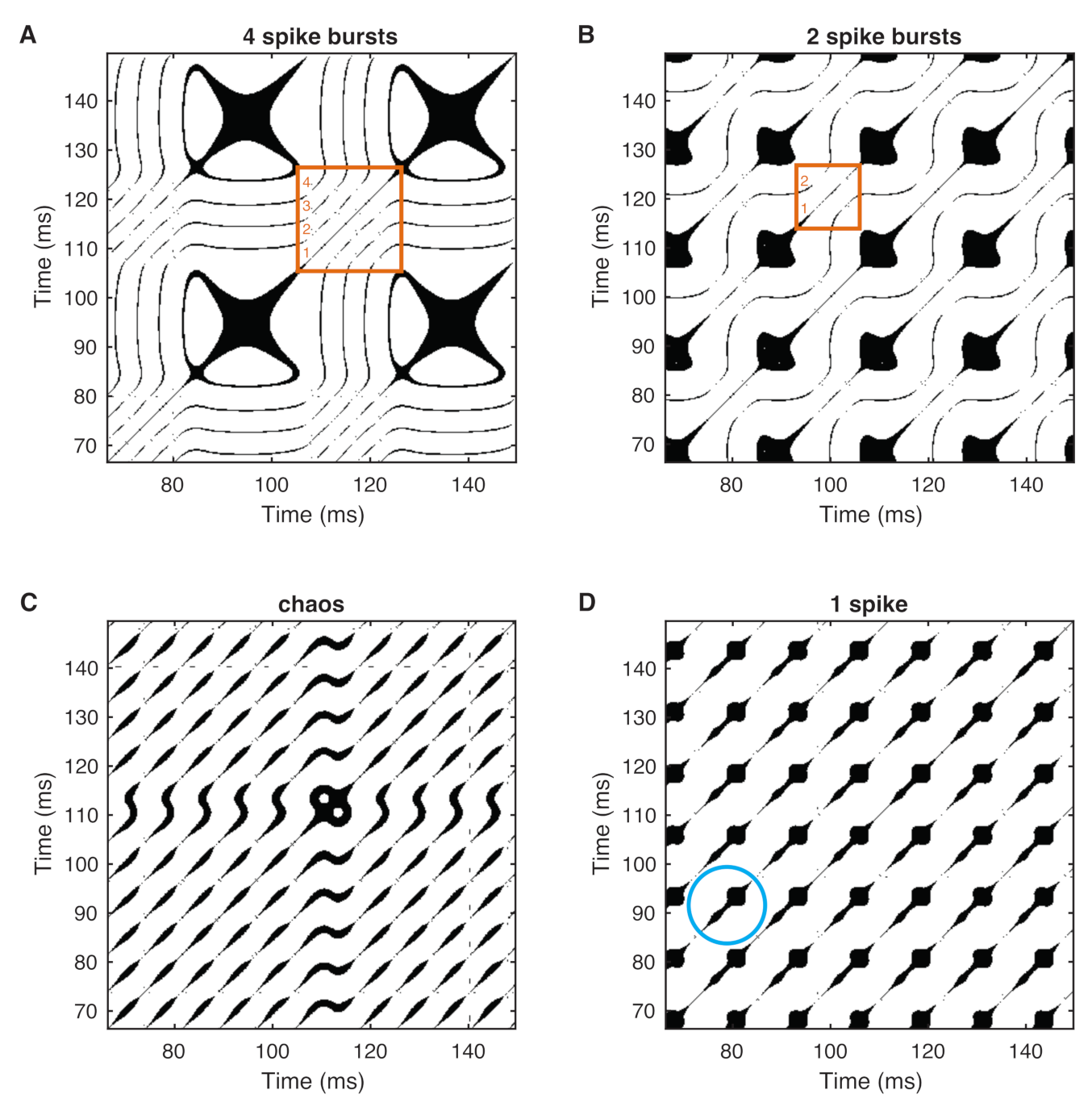
2.2. Bursting Patterns of a Neuron

To explore how the neuron model responds to the externally applied ELF EF, we study the dynamics described by Equations (9) and (10) under the sinusoidal stimulus $v_{\mathrm{e}}$, Equation (6). The simulations are implemented using the 4th-order Runge–Kutta method with a time step of 0.01 ms. Initial conditions are chosen as the resting values of membrane voltage in the absence of stimuli, that is, $v\left(0\right)=-65$ mV and $w\left(0\right)=0$. The length of the time series is 2000 ms. The response of a neuron induced by an EF depends on the EF’s frequency $\omega$ (Figure 1 for $\omega$ in the range $0\le \omega \le 0.5$ rad/ms). The amplitude of the external EF is set very small, $A=0.1$.

The firing pattern of a neuron stimulated by an external EF varies when changing the frequency $\omega$ (Figure 1 and Figure 2). For an ELF EF with very low frequency, the neuron fires periodically. We find n spike bursting states, and the number n can be large. n spike bursting means that we have n action potentials in every stimulus period (Figure 1A–D and Figure 2) for $\omega =[0.001,0.120]$ rad/ms. After this range $\omega$ of n-periodic bursting, the neuron bursts synchronously to the stimulus $\omega =[0.121,0.280]$ rad/ms. After this range of $\omega$, the neuron exhibits a chaotic response (Figure 1E) with $\omega =[0.281,0.320]$ rad/ms where the membrane potential responses are aperiodic and irregular. As $\omega$ is further increased, a mode locking pattern of bursting appears (Figure 1F), finally followed by synchronized firing with only one action potential in every stimulus, which can maintain this state for a long-term frequency band (Figure 1G). Neuron dynamics are obviously very sensitive to the frequency of the stimulus by the ELF EF.

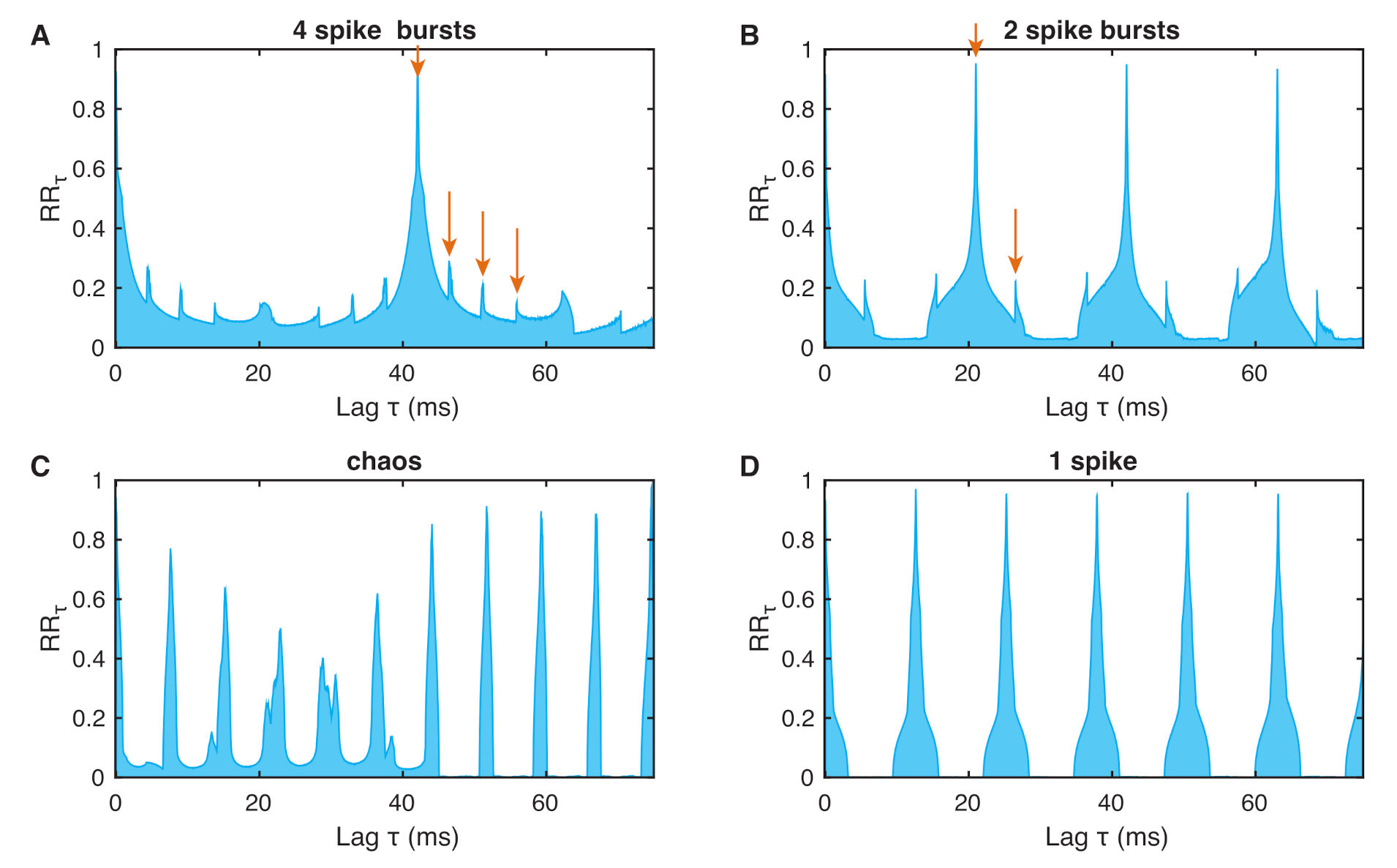
3. Recurrence Quantification Analysis (RQA)

In the following, neuron dynamics will be studied using recurrence quantification analysis (RQA). This method quantifies certain recurrence features of the dynamical system in its corresponding phase space [35,63]. We define a recurrence of a trajectory $\overrightarrow{x}\left(t\right)\in {\mathbb{R}}^m$ (with m the dimension of the system) of a dynamical system by saying that the trajectory has returned at time $t=j$ to the former point in phase space visited at $t=i$ (with $i\in [1,N]$ and N the length of time series) if

$$\begin{array}{c}\hfill R_{i,j}=\mathsf{\Theta }\left(\epsilon -∥\overrightarrow{x}\left(i\right)-\overrightarrow{x}\left(j\right)∥\right)\end{array}$$

(11)

where $\epsilon$ is a pre-defined threshold and $\mathsf{\Theta }\left(·\right)$ is the Heaviside function. We have a matrix of (0, 1), where 1 at (i, j) means that $\overrightarrow{x}\left(i\right)$ and $\overrightarrow{x}\left(j\right)$ are neighbors and 0 means that they are not. The resulting black and white representation of this binary matrix is called a recurrence plot (RP). For the selection of the recurrence threshold $\epsilon$, different strategies are available, depending on the research question [64,65,66,67,68,69]. Here, we use an approach to select $\epsilon$ in a way that ensures a certain recurrence point density. This allows a better comparability between RPs of different systems [68].

The RP method has been intensively studied and applied in the last years. Different measures of complexity have been proposed that can classify different dynamics, identify dynamical transitions, or detect couplings, causality, or synchronization [35].

If not all state variables of the state vector $\overrightarrow{x}$ are available, a phase space reconstruction has to be applied. Here, we use the recently proposed PECUZAL method to reconstruct the phase space trajectories [70]. This method allows us to use multiple embedding delays $\tau$. The embedding parameters are listed in

Table 2. Embedding parameters indicated by the PECUZAL algorithm.

Time Series	Dimension	Delay
4 spike burst ($\omega =0.05$ rad/ms)	3	17, 22
2 spike burst ($\omega =0.10$ rad/ms)	2	16, 20
chaos ($\omega =0.286$ rad/ms)	2	20
1 spike ($\omega =0.5$ rad/ms	2	19

.

RPs of the different bursting neurons represent a typical pattern (Figure 3, using an $\epsilon$ that ensures a recurrence point density of 0.15). Each “dashed-dotted” diagonal line in the RPs corresponds to a spike. For the alternating spiking behavior, we have a set of dashed lines followed by an extended black region (Figure 3A,B). The set of n spikes is well distinguished by the number of dashed lines (see some orange boxes marked in the figure). The block-like black region represents the silent state between each stimulus, which is a period for which the neuron cannot respond to a stimulus. On the small scale, the diagonal lines show some additional patterns, i.e., small structures sitting perpendicularly at these lines or thickenings, similar to bumps or knobs. This is a typical feature of slow–fast systems [71].

In order to go beyond the visual impression of the RP, we use recurrence quantification analysis (RQA) [35,72]. The RQA measures are based on the recurrence point density and the diagonal and vertical line structures of the RP. For example, the recurrence point density $\frac{1}{N^2}\sum R_{i,j}$ corresponds to the probability that a state will recur. The calculation of this measure can also be restricted to a diagonal-wise calculation, i.e., the recurrence point density along a diagonal with distance $\tau$ from the main diagonal $R_{i,i}=1$ [35]. This gives us an estimator of the probability that the system returns to a previous state after time $\tau$ and is called the $\tau$-recurrence rate,

$$\begin{array}{c}\hfill R{R}_{\tau }=\frac{1}{N-\tau }\sum _{i=0}^{N-\tau }{R}_{i,i+\tau }\end{array}$$

(12)

where $\tau$ is the set time and N the total number of points in the phase space. The distance between the peaks in an $R{R}_{\tau }$ plot corresponds to the period length of oscillations or the interspike intervals of spike trains similar to the neuron’s spiking/bursting patterns.

The spike trains of 4 spikes, 2 spikes, chaos, and 1 spike have their specific probability distributions for recurrence after lag $\tau$ (Figure 4). Where the 1-periodic spike occurrence is clearly visible for 1 spike (Figure 4D), the 2 and 4 spikes produce more subtle probability distributions, revealing different periodicities and large blocks between the bursting periods (Figure 4A,B). The $R{R}_{\tau }$ of the chaotic bursting exhibits a more complicated distribution of peaks corresponding to the unpredictable occurrence of spikes (Figure 4C).

4. Coupling of Two Bursting Neurons

4.1. Model and Numerical Simulation

A coupling between ML neurons is realized by a gap junction. We suppose that the two neurons are slightly different by considering different values of $u_2$ and $u_3$ in Equations (4) and (5), i.e., $u_{2,1}=-18.0$ mV and $u_{2,2}=-18.1$ mV, and $u_{3,1}=-12.8$ mV and $u_{3,2}=-10$ mV for neurons 1 and 2, respectively. Moreover, both neurons start using different initial conditions $v_1\left(0\right)=-65.6$ mV and $v_2\left(0\right)=-60$ mV. We integrate the model for 50,000 time steps (with $dt=0.05$) and remove the first 10,000 points as transients. Using the ELF EF frequency that leads to chaotic bursting $\omega =0.286$ rad/ms, the coupled chaotic bursting ML neurons under ELF EF exposure can be expressed as

$$\begin{array}{ccc}\hfill c\frac{d{v}_1}{dt}& =& i_{\mathrm{stim}}-\frac{d\Delta v_1}{dt}-i_{1,\mathrm{fast}}-i_{1,\mathrm{slow}}-i_{1,\mathrm{leak}}-g(v_1-v_2)\hfill \end{array}$$

(13)

$$\begin{array}{ccc}\hfill \frac{d{w}_1}{dt}& =& \phi \frac{m_2\left(v_1\right)-w_1}{b\left(v_1\right)}\hfill \end{array}$$

(14)

$$\begin{array}{ccc}\hfill c\frac{d{v}_2}{dt}& =& i_{\mathrm{stim}}-\frac{d\Delta v_2}{dt}-i_{2,\mathrm{fast}}-i_{2,\mathrm{slow}}-i_{2,\mathrm{leak}}-g(v_2-v_1)\hfill \end{array}$$

(15)

$$\begin{array}{ccc}\hfill \frac{d{w}_2}{dt}& =& \phi \frac{m_2\left(v_2\right)-w_2}{b\left(v_2\right)},\hfill \end{array}$$

(16)

where g is the gap which represents the electrical junction between the neurons. With these two different chaotic neurons, we will now study the phase synchronization between them and focus on the range of weak coupling, i.e., with 500 values of g within the interval $g=[0,0.15]$ (Figure 5).

When bursting begins at the same time in the coupled neurons, we have bursting synchronization irrespective of the neurons’ spiking behaviors within a given burst event. From a dynamical point of view, since we assign a phase that increases by $2\pi$ at each burst event, we regard bursting synchronization as a kind of phase synchronization [73]. Thus, first we will determine the phase of each chaotic bursting neuron. A frequently used approach to calculate the phase of a signal is using the Hilbert transformation [15]

$$\begin{array}{c}\hfill \varphi \left(t\right)=arctan2\left(v_H\left(t\right),v\left(t\right)\right)\end{array}$$

(17)

where $v_H$ is the complex part of the Hilbert transform of the membrane voltage $v\left(t\right)$ and $\varphi \left(t\right)$ increases continually with time. Since chaotic neurons have chaotic spikes, the phase of chaotic neurons changes also chaotically. Unfortunately, this approach does not work well for spiky signals and can cause slipping of the instantaneous phases. Nevertheless, for long-term averages, it provides useful results.

To detect phase synchronization of chaotic coupled neurons and to evaluate the effect of an ELF EF on this synchronization, we first consider the absolute phase difference between the membrane voltage of both neurons without and with applied EF. Phase synchronization occurs if the difference ${\varphi }_1\left(t\right)-{\varphi }_2\left(t\right)$ between the phases of the two neurons does not grow with time [74]. This means that the two neurons, on average, generate spikes almost simultaneously. With the knowledge of the phase $\varphi \left(t\right)$, the frequency $\overline{\omega }\left(t\right)=\frac{d\varphi \left(t\right)}{dt}$ and the mean frequency $\mathsf{\Omega }=〈\frac{d\varphi \left(t\right)}{dt}〉$ can be defined. A weaker form of synchronization is frequency locking. Frequency locking between coupled systems can be measured by the mismatch between the average frequencies $\Delta \mathsf{\Omega }={\mathsf{\Omega }}_1-{\mathsf{\Omega }}_2$, with $\Delta \mathsf{\Omega }\to 0$ for phase locking.

The weakly coupled neurons show frequency locking without ELF EF when the coupling exceeds a critical value (Figure 6). The frequency mismatch $\Delta \mathsf{\Omega }$ between both neurons is constant between $g=0$ (no coupling) and $g=0.025$. After this value, $\Delta \mathsf{\Omega }$ is decreasing and vanishes around $g=0.066$, indicating the onset of synchronization frequency locking between the neurons.

With ELF EF applied, the frequency difference is smaller, even for $g=0$, and decreases much faster than without EF; the neurons become frequency-locked for $g=0.037$ (Figure 6). Thus, in a range of weakly connected neurons, applying an external ELF EF on the chaotic coupled ML neurons enhances frequency-locked synchronization. This confirms earlier findings of synchronized neurons using a different model of weakly connected bursters [24].

Since the firing pattern strongly depends on the amplitude of the ELF EF, we expect that the occurrence of frequency locking also depends on this external stimulus amplitude. In fact, we find that an amplitude value of $A=0.15$ is strong enough to cause a complete synchronization of two neurons even without coupling (Figure 7). Therefore, we select a lower amplitude value of $A=0.1$, where we still have a significant frequency mismatch between the uncoupled neurons. A weak coupling between the neurons leads, finally, to frequency-locked synchronization for lower ELF EF amplitudes.

To test for phase synchronization, i.e., whether the difference ${\varphi }_1\left(t\right)-{\varphi }_2\left(t\right)$ remains constant, we will use an alternative method which can derive the phases of spiky signals in a more reliable way.

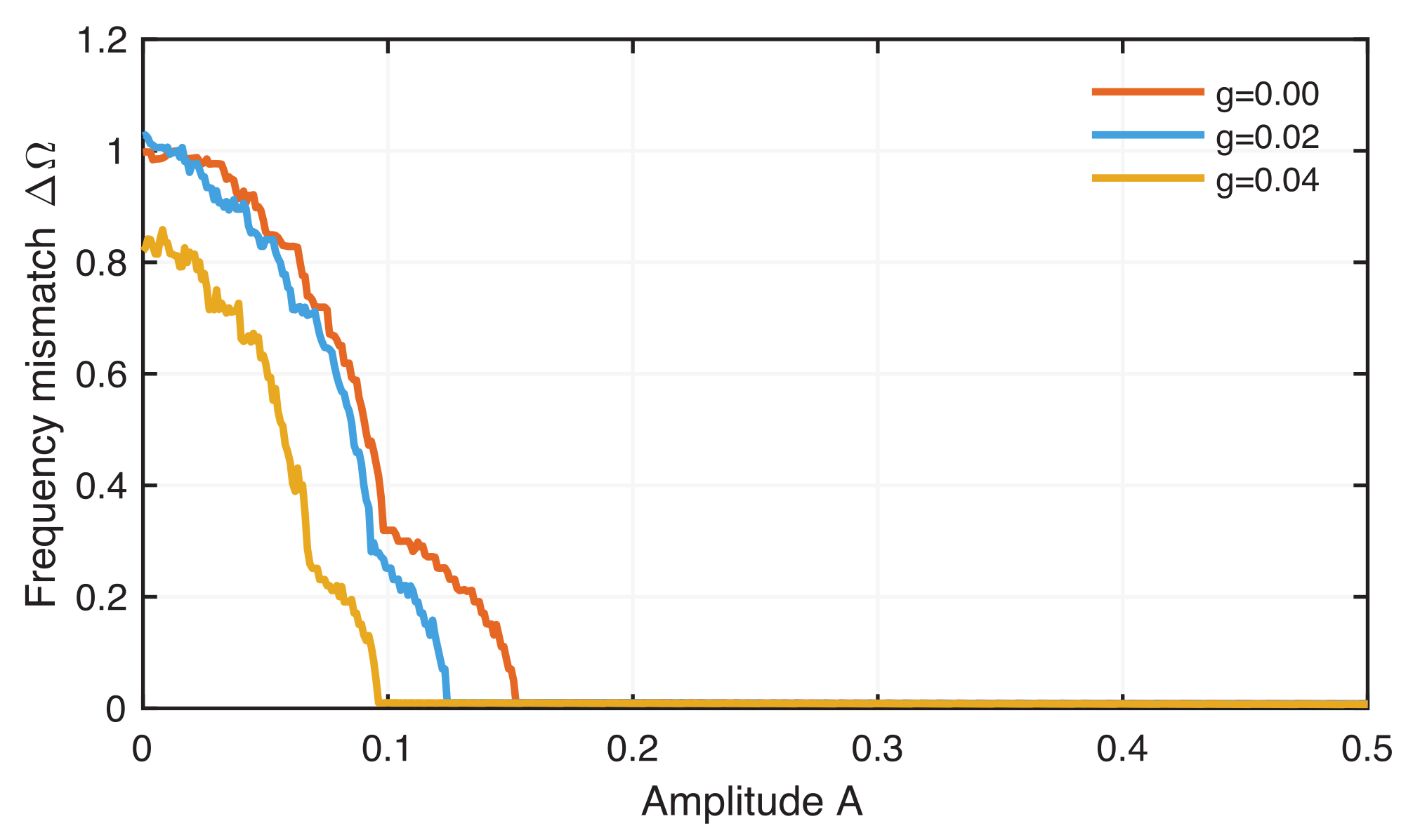
4.2. Phase Synchronization Analysis Using Recurrence Features

Phase synchronization is related to recurrence of states. Therefore, RPs are a natural tool to study phase synchronization [35]. The spiking pattern causes regular and almost periodic occurrence of diagonal line structures in the RPs (Figure 8). Here, we use a recurrence threshold $\epsilon$ to ensure a recurrence point density of 0.1. Although we notice a certain amount of similarity between the RPs of neuron 1 and neuron 2 in the nonsynchronized regime, we still see deviations in the line patterns of the RP of neuron 2 (Figure 8A,B). In contrast, the RPs of neuron 1 and neuron 2 for the in-phase synchronized regime show a striking similarity (Figure 8C,D).

The vertical distance between these diagonal line structures is related to the phase. Therefore, we can use the density of recurrence points along diagonals parallel to the main diagonal, the $\tau$-recurrence rate $R{R}_{\tau }$, Equation (12), as an estimator of the phase distribution and compare it between different systems. For two nonsynchronized systems, the recurrence probabilities should differ significantly (Figure 9A). During phase synchronization, $R{R}_{\tau }$ should have high probabilities at the same $\tau$ values; thus, the shape of $R{R}_{\tau }$ should be very similar (Figure 9B). Therefore, $R{R}_{\tau }$ has been used to construct a measure for phase synchronization between two signals $x_1$ and $x_2$ by calculating the Pearson correlation of probability of recurrence (CPR) between $R{R}_{\tau }^{x_1}$ and $R{R}_{\tau }^{x_2}$ [34]

$$CP{R}^{\mathrm{P}}=\frac{\mathrm{cov}(R{R}_{\tau }^{x_1},R{R}_{\tau }^{x_2})}{{\sigma }_{R{R}_{\tau }^{x_1}}{\sigma }_{R{R}_{\tau }^{x_2}}},$$

(18)

with ${\sigma }_{R{R}_{\tau }}$ the standard deviation of the corresponding $R{R}_{\tau }$ series. CPR values of 1 would then correspond to phase synchronization and 0 to no synchronization. Here, it is important to remove the first peak in $R{R}_{\tau }$ close to $\tau =0$ because these values correspond to the main diagonal in the RP present in all systems [50]. Therefore, this first peak would indicate some kind of similarity between $R{R}_{\tau }\left(x_1\right)$ and $R{R}_{\tau }\left(x_2\right)$ even for completely desynchronized systems. Such exclusion of the first part of the $R{R}_{\tau }$ series corresponds to applying a Theiler window [75]. Here we used a Theiler window of 25 mS.

Another concern on calculating the CPR measure using Equation (18) is the spiky shape of the $R{R}_{\tau }$ series, biasing the Pearson correlation estimation. As an alternative, we could use the Spearman rank correlation instead of the Pearson correlation,

$$CP{R}^{\mathrm{S}}=\frac{\mathrm{cov}\left(\mathrm{R}\left(R{R}_{\tau }^{x_1}\right),\mathrm{R}\left(R{R}_{\tau }^{x_2}\right)\right)}{{\sigma }_{\mathrm{R}\left(R{R}_{\tau }^{x_1}\right)}{\sigma }_{\mathrm{R}\left(R{R}_{\tau }^{x_2}\right)}},$$

(19)

with the $R{R}_{\tau }$ series converted to the ranks $\mathrm{R}\left(R{R}_{\tau }\right)$. This correlation measure is expected to work better for non-normal distributed data, as the $R{R}_{\tau }$ series would be.

Both CPR measures clearly show the onset of phase synchronization at $g=0.066$ for neurons without ELF EF and at $g=0.037$ for neurons with ELF EF (Figure 10). There are some differences between $CP{R}^{\mathrm{P}}$ and $CP{R}^{\mathrm{S}}$. During phase synchronization, $CP{R}^{\mathrm{P}}$ is almost 1, but $CP{R}^{\mathrm{S}}$ is slightly below 1, even more obvious for the coupled neurons without ELF EF. However, for phase synchronization, we would expect to have a CPR value of 1. Moreover, the transition from a nonsynchronized regime to a synchronized regime is not as abrupt as indicated by $\Delta \mathsf{\Omega }$ (Figure 6), but $CP{R}^{\mathrm{S}}$ changes almost abruptly from very low values to very large values, whereby $CP{R}^{\mathrm{P}}$ shows a more gradual increase (and even step-wise increase for $A=0$). This finding indicates that the Spearman-based CPR is obviously not a better choice than the Pearson-based CPR measure.

The $R{R}_{\tau }$ series represents probabilities of recurrence. Therefore, it seems more natural to use a measure that can directly quantify the difference between probability populations, such as Kullback–Leibler distance [76] or Hellinger distance [77]. Here we test the use of the Hellinger distance

$$H(R{R}_{\tau }^{x_1},R{R}_{\tau }^{x_2})=\frac{1}{\sqrt{2}}∥\sqrt{R{R}_{\tau }^{x_1}}-\sqrt{R{R}_{\tau }^{x_2}}∥,$$

(20)

which corresponds to the Euclidean norm of the square root distances between the $R{R}_{\tau }$ series of the two signals. Values of H close to 0 indicate phase transition, whereas values close to 1 indicate nonsynchronized regimes.

To assess whether the variation of H indeed reveals phase synchronization, we use a simple block shuffling approach to test the null hypothesis that the signals are not synchronized. Block shuffling splits a time series into a number of blocks (here, we used five blocks) of equal width at random indices and randomly concatenates these blocks to create a new surrogate time series. Such surrogates preserve short-term temporal properties but destroy long-term dynamical information and, thus, correlations when compared with another signal. The distribution $p\left(H\right)$ derived from the ensemble of surrogates is then used to define the confidence limit of 95% (simply by using the 95% quantile of this test distribution $p\left(H\right)$). Considering $A=0$, we find the confidence limit by $H_{0.95}$ as 0.17. Values of H below this value can be considered to represent phase synchronization.

The measure H indicates the transition from the nonsynchronous to the phase synchronization regime of the two weakly coupled neurons (Figure 11). The change in H is significant. Moreover, the variation in H over increasing coupling strength g reveals the more gradual change to the phase synchronization as well as the step-like transition to phase synchronization for the situation without ELF EF caused by phase jumps.

5. Conclusions

The synchronization of weakly coupled Morris–Lecar neurons under common external forcing has been studied previously. For example, Kitajima and Kurths [21] used interspike intervals (to study frequency locking) and Yi et al. [62] considered the average firing rate. In general, the numerical calculation of the phases of spiky signals using the Hilbert transform is problematic. An alternative way to identify the phases in dynamical systems is to use recurrence plots [34]. This method can find phases for noncoherent and spiky signals. We, therefore, used a recurrence-based approach, which decodes the phase in terms of specific recurrence patterns in the recurrence plot, and demonstrated its potential for the study of spiking patterns of neurons.

In this work, the spiking patterns of Morris–Lecar neurons under ELF sinusoidal EF and the synchronization of two neurons weakly coupled with gap junction under ELF EF were investigated using this recurrence-based approach. The representation of the dynamics of the neurons’ membrane voltages by recurrence plots provided a convenient approach to compare the recurrence features of their spiking patterns. Various spiking patterns, such as periodic and chaotic bursting and periodic spikes, were observed. The spiking patterns were found to be very sensitive to changes of the stimulus frequency.

Moreover, the recurrence approach allows us to consider phase differences between the spiking patterns in a more robust way than the frequently used Hilbert transform. We have introduced an alternative measure for testing phase synchronization using recurrences. Instead of comparing the probabilities of recurrences (as represented by the $\tau$-recurrence rate) by correlation coefficients, we suggest to use the Hellinger distance as a more natural measure because it quantifies the differences between probabilities. The typically used Pearson correlation is biased because the $\tau$-recurrence rate does not follow a normal distribution. The Spearman rank correlation could be an alternative, but we found additional bias due the large number of zeros in the $\tau$-recurrence rate series.

By using recurrence-based synchronization measures, we found that even without external EF, phase synchronization of two ML neurons can occur for a range of values of coupling strength. Moreover, phase synchronization can be enhanced by an additional external EF. This physiological behavior might be of importance for the functioning of the brain when exposed to electromagnetic fields, such as by power lines, electrical equipment, or cellular radio towers.

References

1. Adrian, E.D. The Mechanism of Nervous Action, Electrical Studies of the Neurone; University of Pennsylvania Press: Philadelphia, PA, USA, 1932. [Google Scholar]
2. Huang, K.; Li, Y.; Yang, C.; Gu, M. The dynamic principle of interaction between weak electromagnetic fields and living system–Interference of electromagnetic waves in dynamic metabolism. Chin. J. Med. Phys. 1996, 14, 205–207. [Google Scholar]
3. Reato, D.; Rahman, A.; Bikson, M.; Parra, L.C. Low-Intensity Electrical Stimulation Affects Network Dynamics by Modulating Population Rate and Spike Timing. J. Neurosci. 2010, 30, 15067–15079. [Google Scholar] [CrossRef] [Green Version]
4. Opitz, A.; Falchier, A.; Yan, C.G.; Yeagle, E.M.; Linn, G.S.; Megevand, P.; Thielscher, A.; Deborah, A.R.; Milham, M.P.; Mehta, A.D.; et al. Spatiotemporal structure of intracranial electric fields induced by transcranial electric stimulation in humans and nonhuman primates. Sci. Rep. 2016, 6, 31236. [Google Scholar] [CrossRef] [Green Version]
5. Huang, Y.; Liu, A.A.; Lafon, B.; Friedman, D.; Dayan, M.; Wang, X.; Bikson, M.; Doyle, W.K.; Devinsky, O.; Parra, L.C. Measurements and models of electric fields in the in vivo human brain during transcranial electric stimulation. eLife 2017, 6, e18834. [Google Scholar] [CrossRef]
6. Savitz, D.A.; Loomis, D.P.; Tse, C.K.J. Electrical occupations and neurodegenerative disease: Analysis of US mortality data. Arch. Environ. Health Int. J. 1998, 53, 71–74. [Google Scholar] [CrossRef]
7. Johansen, C. Exposure to electromagnetic fields and risk of central nervous system disease in utility workers. Epidemiology 2000, 11, 539–543. [Google Scholar] [CrossRef]
8. Radman, T.; Su, Y.; An, J.H.; Parra, L.C.; Bikson, M. Spike timing amplifies the effect of electric fields on neurons: Implications for endogenous field effects. J. Neurosci. 2007, 27, 3030–3036. [Google Scholar] [CrossRef]
9. Nkomidio, A.M.; Woafo, P. Effects of imperfection of ionic channels and exposure to electromagnetic fields on the generation and propagation of front waves in nervous fibre. Commun. Nonlinear Sci. Numer. Simul. 2010, 15, 2350–2360. [Google Scholar] [CrossRef]
10. Eichwald, C.; Kaiser, F. Model for external influences on cellular signal transduction pathways including cytosolic calcium oscillations. Bioelectromagnetics 1995, 16, 75–85. [Google Scholar] [CrossRef]
11. Huang, C.; Xu, B.; Lin, J. Effects of extremely low frequency magnetic fields on hormone-induced cytosolic calcium oscillations. Shengwu Wuli Xuebao 1998, 15, 543–546. [Google Scholar]
12. Wertheimer, N.; Leeper, E. Electrical wiring configurations and childhood cancer. Am. J. Epidemiol. 1979, 109, 273–284. [Google Scholar] [CrossRef] [PubMed]
13. Moulder, J.E. Power-frequency fields and cancer. Crit. Rev. Biomed. Eng. 1998, 26, 1–116. [Google Scholar] [CrossRef] [PubMed]
14. Stuchly, M.A.; Dawson, T.W. Interaction of low-frequency electric and magnetic fields with the human body. Proc. IEEE 2000, 88, 643–664. [Google Scholar] [CrossRef]
15. Pikovsky, A.; Rosenblum, M.; Kurths, J. Synchronization—A Universal Concept in Nonlinear Sciences; Cambridge University Press: Cambridge, UK, 2001. [Google Scholar]
16. Golomb, D.; Rinzel, J. Clustering in globally coupled inhibitory neurons. Phys. D Nonlinear Phenom. 1994, 72, 259–282. [Google Scholar] [CrossRef]
17. Dayan, P.; Abbott, L. Theoretical Neuroscience: Computational and Mathematical Modeling of Neural Systems; MIT Press: Cambridge, MA, USA, 2001. [Google Scholar]
18. Gray, C.M.; König, P.; Engel, A.K.; Singer, W. Oscillatory responses in cat visual cortex exhibit inter-columnar synchronization which reflects global stimulus properties. Nature 1989, 338, 334–337. [Google Scholar] [CrossRef]
19. Morris, C.; Lecar, H. Voltage oscillations in the barnacle giant muscle fiber. Biophys. J. 1981, 35, 193. [Google Scholar] [CrossRef] [Green Version]
20. Rinzel, J.; Ermentrout, G.B. Analysis of Neural Excitability and Oscillations. In Methods in Neuronal Modeling; Koch, C., Segev, I., Eds.; MIT Press: Cambridge, MA, USA, 1989; pp. 251–291. [Google Scholar]
21. Kitajima, H.; Kurths, J. Forced synchronization in Morris–Lecar neurons. Int. J. Bifurc. Chaos 2007, 17, 3523–3528. [Google Scholar] [CrossRef] [Green Version]
22. Hoppensteadt, F.C.; Izhikevich, E.M. Weakly Connected Neural Networks; Springer: New York, NY, USA, 1997. [Google Scholar]
23. Hoppensteadt, F.C.; Izhikevich, E.M. Synaptic organizations and dynamical properties of weakly connected neural oscillators II. Learning phase information. Biol. Cybern. 1996, 75, 129–135. [Google Scholar] [CrossRef]
24. Izhikevich, E.M. Synchronization of elliptic bursters. Siam Rev. 2001, 43, 315–344. [Google Scholar] [CrossRef] [Green Version]
25. Gutfreund, Y.; Yarom, Y.; Segev, I. Subthreshold oscillations and resonant frequency in guinea-pig cortical neurons: Physiology and modelling. J. Physiol. 1995, 483, 621–640. [Google Scholar] [CrossRef]
26. Hutcheon, B.; Miura, R.M.; Puil, E. Subthreshold membrane resonance in neocortical neurons. J. Neurophysiol. 1996, 76, 683–697. [Google Scholar] [CrossRef] [PubMed] [Green Version]
27. Hu, H.; Vervaeke, K.; Storm, J.F. Two forms of electrical resonance at theta frequencies, generated by M-current, h-current and persistent Na + current in rat hippocampal pyramidal cells. J. Physiol. 2002, 545, 783–805. [Google Scholar] [CrossRef] [PubMed]
28. Giocomo, L.M.; Zilli, E.A.; Fransén, E.; Hasselmo, M.E. Temporal Frequency of Subthreshold Oscillations Scales with Entorhinal Grid Cell Field Spacing. Science 2007, 315, 1719–1722. [Google Scholar] [CrossRef] [PubMed] [Green Version]
29. Vera, J.; Pezzoli, M.; Pereira, U.; Bacigalupo, J.; Sanhueza, M. Electrical Resonance in the θ Frequency Range in Olfactory Amygdala Neurons. PLoS ONE 2014, 9, e85826. [Google Scholar] [CrossRef] [Green Version]
30. Fischer, L.; Leibold, C.; Felmy, F. Resonance Properties in Auditory Brainstem Neurons. Front. Cell. Neurosci. 2018, 12, 8. [Google Scholar] [CrossRef] [Green Version]
31. Bennett, M.V.; Zukin, R. Electrical Coupling and Neuronal Synchronization in the Mammalian Brain. Neuron 2004, 41, 495–511. [Google Scholar] [CrossRef] [Green Version]
32. Dong, A.; Liu, S.; Li, Y. Gap Junctions in the Nervous System: Probing Functional Connections Using New Imaging Approaches. Front. Cell. Neurosci. 2018, 12, 320. [Google Scholar] [CrossRef]
33. Sabatini, B.L.; Regehr, W.G. Timing of neurotransmission at fast synapses in the mammalian brain. Nature 1996, 384, 170–172. [Google Scholar] [CrossRef]
34. Romano, M.C.; Thiel, M.; Kurths, J.; Kiss, I.Z.; Hudson, J.L. Detection of synchronization for non-phase-coherent and non-stationary data. Europhys. Lett. 2005, 71, 466–472. [Google Scholar] [CrossRef] [Green Version]
35. Marwan, N.; Romano, M.C.; Thiel, M.; Kurths, J. Recurrence Plots for the Analysis of Complex Systems. Phys. Rep. 2007, 438, 237–329. [Google Scholar] [CrossRef]
36. Marwan, N. A Historical Review of Recurrence Plots. Eur. Phys. J. Spec. Top. 2008, 164, 3–12. [Google Scholar] [CrossRef] [Green Version]
37. Babloyantz, A. Evidence for slow brain waves: A dynamical approach. Electroencephalogr. Clin. Neurophysiol. 1991, 78, 402–405. [Google Scholar] [CrossRef]
38. Song, I.H.; Lee, D.S.; Kim, S.I. Recurrence quantification analysis of sleep electoencephalogram in sleep apnea syndrome in humans. Neurosci. Lett. 2004, 366, 148–153. [Google Scholar] [CrossRef]
39. Bergner, A.; Romano, M.C.; Kurths, J.; Thiel, M. Synchronization analysis of neuronal networks by means of recurrence plots. In Lectures in Supercomputational Neurosciences; Beim Graben, P., Zhou, C., Thiel, M., Kurths, J., Eds.; Understanding Complex Systems; Springer: Berlin/ Heidelberg, Germany, 2008; pp. 177–191. [Google Scholar] [CrossRef]
40. Ouyang, G.; Li, X.; Dang, C.; Richards, D.A. Using recurrence plot for determinism analysis of EEG recordings in genetic absence epilepsy rats. Clin. Neurophysiol. 2008, 119, 1747–1755. [Google Scholar] [CrossRef] [PubMed]
41. Budzinski, R.C.; Boaretto, B.R.R.; Prado, T.L.; Lopes, S.R. Phase synchronization and intermittent behavior in healthy and Alzheimer-affected human-brain-based neural network. Phys. Rev. 2019, 99, 022402. [Google Scholar] [CrossRef] [PubMed]
42. Rodriguez-Sabate, C.; Rodriguez, M.; Morales, I. Studying the functional connectivity of the primary motor cortex with the binarized cross recurrence plot: The influence of Parkinson’s disease. PLoS ONE 2021, 16, e0252565. [Google Scholar] [CrossRef] [PubMed]
43. Mendonça, P.R.F.; Vargas-Caballero, M.; Erdélyi, F.; Szabó, G.; Paulsen, O.; Robinson, H.P.C. Stochastic and deterministic dynamics of intrinsically irregular firing in cortical inhibitory interneurons. eLife 2016, 5, e16475. [Google Scholar] [CrossRef] [PubMed]
44. Boaretto, B.R.R.; Budzinski, R.C.; Prado, T.L.; Kurths, J.; Lopes, S.R. Neuron dynamics variability and anomalous phase synchronization of neural networks. Chaos 2018, 28, 106304. [Google Scholar] [CrossRef]
45. Tibau, E.; Soriano, J. Analysis of spontaneous activity in neuronal cultures through recurrence plots: Impact of varying connectivity. Eur. Phys. J. Spec. Top. 2018, 227, 999–1014. [Google Scholar] [CrossRef]
46. Marwan, N.; Thiel, M.; Nowaczyk, N.R. Cross Recurrence Plot Based Synchronization of Time Series. Nonlinear Process. Geophys. 2002, 9, 325–331. [Google Scholar] [CrossRef]
47. Hirata, Y.; Aihara, K. Identifying hidden common causes from bivariate time series: A method using recurrence plots. Phys. Rev. E 2010, 81, 016203. [Google Scholar] [CrossRef] [PubMed]
48. Astakhov, S.V.; Dvorak, A.; Anishchenko, V.S. Influence of chaotic synchronization on mixing in the phase space of interacting systems. Chaos 2013, 23, 013103. [Google Scholar] [CrossRef] [PubMed]
49. Konvalinka, I.; Xygalatas, D.; Bulbulia, J.; Schjodt, U.; Jegindø, E.M.; Wallot, S.; Van Orden, G.C.; Roepstorff, A. Synchronized arousal between performers and related spectators in a fire-walking ritual. Proc. Natl. Acad. Sci. USA 2011, 108, 8514–8519. [Google Scholar] [CrossRef] [PubMed] [Green Version]
50. Goswami, B.; Ambika, G.; Marwan, N.; Kurths, J. On interrelations of recurrences and connectivity trends between stock indices. Physica A 2012, 391, 4364–4376. [Google Scholar] [CrossRef] [Green Version]
51. Ramos, A.M.T.; Builes-Jaramillo, A.; Poveda, G.; Goswami, B.; Macau, E.E.N.; Kurths, J.; Marwan, N. Recurrence measure of conditional dependence and applications. Phys. Rev. E 2017, 95, 052206. [Google Scholar] [CrossRef] [Green Version]
52. Hobbs, B.; Ord, A. Nonlinear dynamical analysis of GNSS data: Quantification, precursors and synchronisation. Prog. Earth Planet. Sci. 2018, 5, 36. [Google Scholar] [CrossRef] [Green Version]
53. Godavarthi, V.; Pawar, S.A.; Unni, V.R.; Sujith, R.I.; Marwan, N.; Kurths, J. Coupled interaction between unsteady flame dynamics and acoustic field in a turbulent combustor. Chaos 2018, 28, 113111. [Google Scholar] [CrossRef]
54. Schinkel, S.; Zamora-López, G.; Dimigen, O.; Sommer, W.; Kurths, J. Functional network analysis reveals differences in the semantic priming task. J. Neurosci. Methods 2011, 197, 333–339. [Google Scholar] [CrossRef]
55. Rangaprakash, D. Connectivity analysis of multichannel EEG signals using recurrence based phase synchronization technique. Comput. Biol. Med. 2014, 46, 11–21. [Google Scholar] [CrossRef]
56. Izhikevich, E.M. Neural exciability, spiking and bursting. Int. J. Bifurc. Chaos 2000, 10, 1171–1266. [Google Scholar] [CrossRef] [Green Version]
57. Prescott, S.A.; De Koninck, Y.; Sejnowski, T.J. Biophysical basis for three distinct dynamical mechanisms of action potential initiation. PLoS Comput. Biol. 2008, 4, e1000198. [Google Scholar] [CrossRef] [PubMed] [Green Version]
58. Orr, D.; Ermentrout, B. Synchronization of oscillators via active media. Phys. Rev. E 2019, 99, 052218. [Google Scholar] [CrossRef] [PubMed] [Green Version]
59. Attwell, D. Interaction of low frequency electric fields with the nervous system: The retina as a model system. Radiat. Prot. Dosim. 2003, 106, 341–348. [Google Scholar] [CrossRef] [PubMed]
60. Bédard, C.; Kröger, H.; Destexhe, A. Model of low-pass filtering of local field potentials in brain tissue. Phys. Rev. E 2006, 73, 051911. [Google Scholar] [CrossRef] [PubMed] [Green Version]
61. Modolo, J.; Thomas, A.; Stodilka, R.; Prato, F.; Legros, A. Modulation of neuronal activity with extremely low-frequency magnetic fields: Insights from biophysical modeling. In Proceedings of the IEEE Fifth International Conference on Bio-Inspired Computing: Theories and Applications (BIC-TA 2010), Changsha, China, 23–26 September 2010. [Google Scholar]
62. Yi, G.S.; Wang, J.; Han, C.X.; Deng, B.; Wei, X.L. Spiking patterns of a minimal neuron to ELF sinusoidal electric field. Appl. Math. Model. 2012, 36, 3673–3684. [Google Scholar] [CrossRef]
63. Eckmann, J.P.; Oliffson Kamphorst, S.; Ruelle, D. Recurrence Plots of Dynamical Systems. Europhys. Lett. 1987, 4, 973–977. [Google Scholar] [CrossRef] [Green Version]
64. Matassini, L.; Kantz, H.; Hołyst, J.A.; Hegger, R. Optimizing of recurrence plots for noise reduction. Phys. Rev. E 2002, 65, 021102. [Google Scholar] [CrossRef] [Green Version]
65. Marwan, N. How to avoid potential pitfalls in recurrence plot based data analysis. Int. J. Bifurc. Chaos 2011, 21, 1003–1017. [Google Scholar] [CrossRef] [Green Version]
66. beim Graben, P.; Hutt, A. Detecting Recurrence Domains of Dynamical Systems by Symbolic Dynamics. Phys. Rev. Lett. 2013, 110, 154101. [Google Scholar] [CrossRef]
67. Vega, I.; Schütte, C.; Conrad, T.O.F. Finding metastable states in real-world time series with recurrence networks. Phys. A 2016, 445, 1–17. [Google Scholar] [CrossRef] [Green Version]
68. Kraemer, K.H.; Donner, R.V.; Heitzig, J.; Marwan, N. Recurrence threshold selection for obtaining robust recurrence characteristics in different embedding dimensions. Chaos 2018, 28, 085720. [Google Scholar] [CrossRef] [PubMed]
69. Andreadis, I.; Fragkou, A.; Karakasidis, T. On a topological criterion to select a recurrence threshold. Chaos 2020, 30, 013124. [Google Scholar] [CrossRef] [PubMed]
70. Kraemer, K.H.; Datseris, G.; Kurths, J.; Kiss, I.Z.; Ocampo-Espindola, J.L.; Marwan, N. A unified and automated approach to attractor reconstruction. New J. Phys. 2021, 23, 033017. [Google Scholar] [CrossRef]
71. Kasthuri, P.; Pavithran, I.; Krishnan, A.; Pawar, S.A.; Sujith, R.I.; Gejji, R.; Anderson, W.; Marwan, N.; Kurths, J. Recurrence analysis of slow–fast systems. Chaos 2020, 30, 063152. [Google Scholar] [CrossRef]
72. Zbilut, J.P.; Webber, C.L., Jr. Embeddings and delays as derived from quantification of recurrence plots. Phys. Lett. A 1992, 171, 199–203. [Google Scholar] [CrossRef]
73. Ivanchenko, M.V.; Osipov, G.V.; Shalfeev, V.D.; Kurths, J. Phase synchronization in ensembles of bursting oscillators. Phys. Rev. Lett. 2004, 93, 134101. [Google Scholar] [CrossRef]
74. Rosenblum, M.G.; Pikovsky, A.S.; Kurths, J. Phase synchronization of chaotic oscillators. Phys. Rev. Lett. 1996, 76, 1804. [Google Scholar] [CrossRef]
75. Theiler, J. Spurious dimension from correlation algorithms applied to limited time-series data. Phys. Rev. A 1986, 34, 2427–2432. [Google Scholar] [CrossRef]
76. Amari, S. Information Geometry and Its Applications; Springer: Tokyo, Japan, 2016; Volume 194. [Google Scholar] [CrossRef]
77. Pollard, D. Densities and derivatives. In A User’s Guide to Measure Theoretic Probability; Cambridge University Press: Cambridge, UK, 2001; pp. 53–76. [Google Scholar] [CrossRef]
Figure 1. Spiking patterns of ML neuron membrane voltage under an external EF for different frequencies: (A) ω = 0.02 rad/ms, (B) ω = 0.05 rad/ms, (C) ω = 0.06 rad/ms, (D) ω = 0.10 rad/ms, (E) ω = 0.286 rad/ms, (F) ω = 0.32 rad/ms, and (G) ω = 0.5 rad/ms.
Entropy 24 00235 g001
Figure 2. Bifurcation diagram of ML neuron dynamics under an external EF for varying frequencies ω (based on interspike intervals of the membrane voltage). For better visibility of the dynamics for larger ω , the y-axis was bounded to 250 ms.
Entropy 24 00235 g002
Figure 3. RPs of the membrane voltage v of selected bursting neurons: (A) 4 spike burst ( ω = 0.05 rad/ms), (B) 2 spike burst ( ω = 0.10 rad/ms), (C) chaos ( ω = 0.286 rad/ms), and (D) 1 spike ( ω = 0.5 rad/ms). Diagonal lines represent the spikes, the larger extended structures represent the “silent” epochs, and the structures perpendicular to the diagonal lines and small thickenings represent the slow–fast dynamics (blue circle in (D)). The orange boxes in (A,B) mark a sequence of diagonal lines. The number of diagonal lines counted from the main diagonal of such a box towards the corner of this box represents the number of spikes within this period. Recurrence threshold ε is selected to ensure a recurrence point density of 0.15.
Entropy 24 00235 g003
Figure 4. Probability of recurrence after time τ ( τ -recurrence rate) for the bursting neurons as shown in Figure 3: (A) 4 spike burst, (B) 2 spike burst, (C) chaos, and (D) 1 spike. The n bursts are visible as the rather thin side peaks of the main peaks (in addition to the main peak).
Entropy 24 00235 g004
Figure 5. Spiking pattern in the membrane voltage of two weakly coupled neurons in an ELF EF in chaotic regime ( ω = 0.286 ) with (A) no synchronization with g = 0.01 and (B) phase synchronization with g = 0.04 .
Entropy 24 00235 g005
Figure 6. Frequency mismatch between chaotic coupled neurons for increasing coupling g without external EF (red) and with external EF where A = 0.1 and ω = 0.286 (blue).
Entropy 24 00235 g006
Figure 7. Frequency mismatch between chaotic coupled neurons for increasing amplitude A and for different coupling strengths g.
Entropy 24 00235 g007
Figure 8. Recurrence plots of the membrane voltage for weakly coupled neurons as shown in Figure 5 for (A,B) no synchronization, g = 0.01 , and (C,D) phase synchronization, g = 0.04 . Embedding parameters were estimated using the PECUZAL method [70]; the recurrence threshold is selected to ensure a recurrence rate of R R = 0.1 .
Entropy 24 00235 g008
Figure 9. τ -recurrence rate for weakly coupled neurons as shown in Figure 5 and Figure 8 for (A) no synchronization, g = 0.01 , and (B) phase synchronization, g = 0.04 . For phase synchronization, the τ -recurrence rate series for both neurons are almost completely overlapping.
Entropy 24 00235 g009
Figure 10. Correlation of probability of recurrence CPR based on Pearson (dotted) and Spearman (line) correlations indicating the onset of phase synchronization between chaotic coupled neurons without external EF (red) and with external EF where A = 0.1 and ω = 0.286 (blue).
Entropy 24 00235 g010
Figure 11. Hellinger distance of the τ -recurrence rate indicating the onset of phase synchronization between chaotic coupled neurons without external EF (red) and with external EF where A = 0.1 and ω = 0.286 (blue). A drop of H below the confidence limit of 95% (dotted line) represents the significance of this finding.
Entropy 24 00235 g011