
Analysis of Individual High-Frequency Traders’ Buy–Sell Order Strategy Based on Multivariate Hawkes Process


Abstract
:1. Introduction
2. Data
2.1. EBS Market Data Description
2.2. Definition of HFTs
2.3. Basic Properties of HFTs
3. Method
3.1. Model
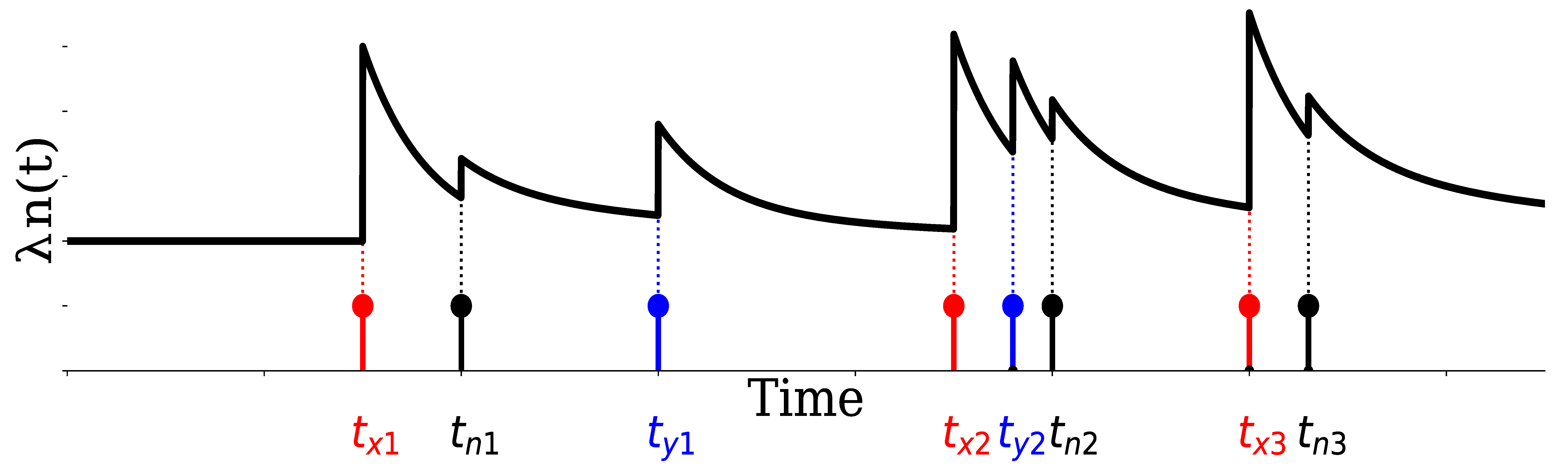
3.1.1. Mathematical Notation
3.1.2. Overview of Hawkes Process
3.1.3. Trader Model
3.2. Parameter Estimation Using Maximum Likelihood Estimation
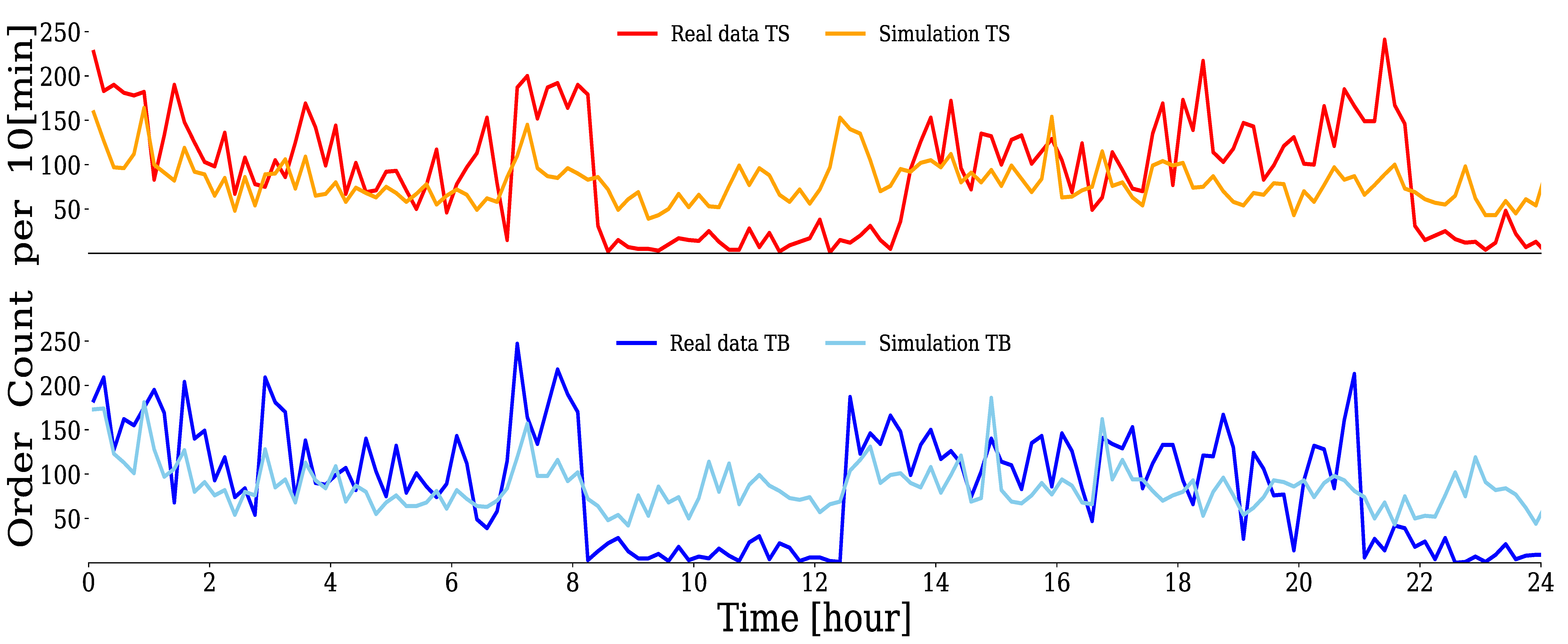
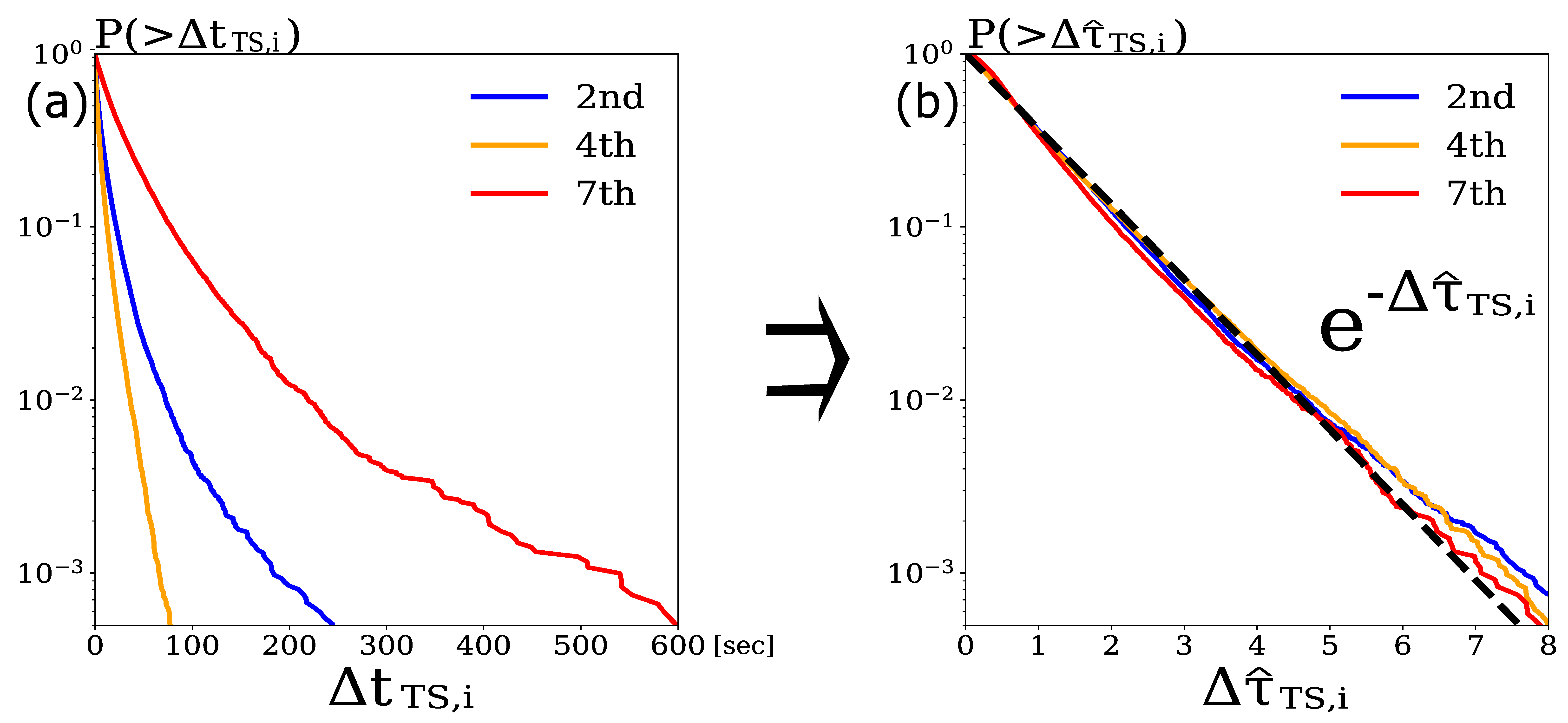
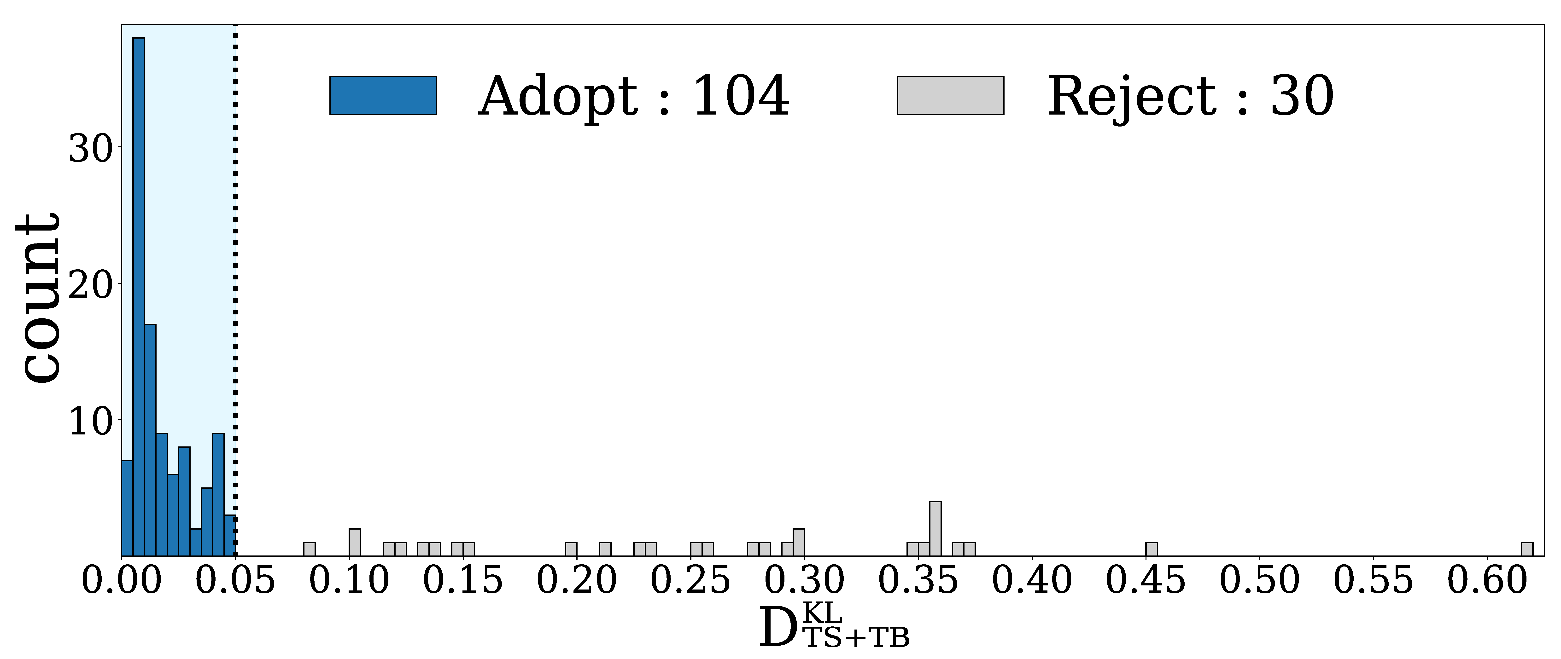
3.3. Validity of Estimation Results
4. Results
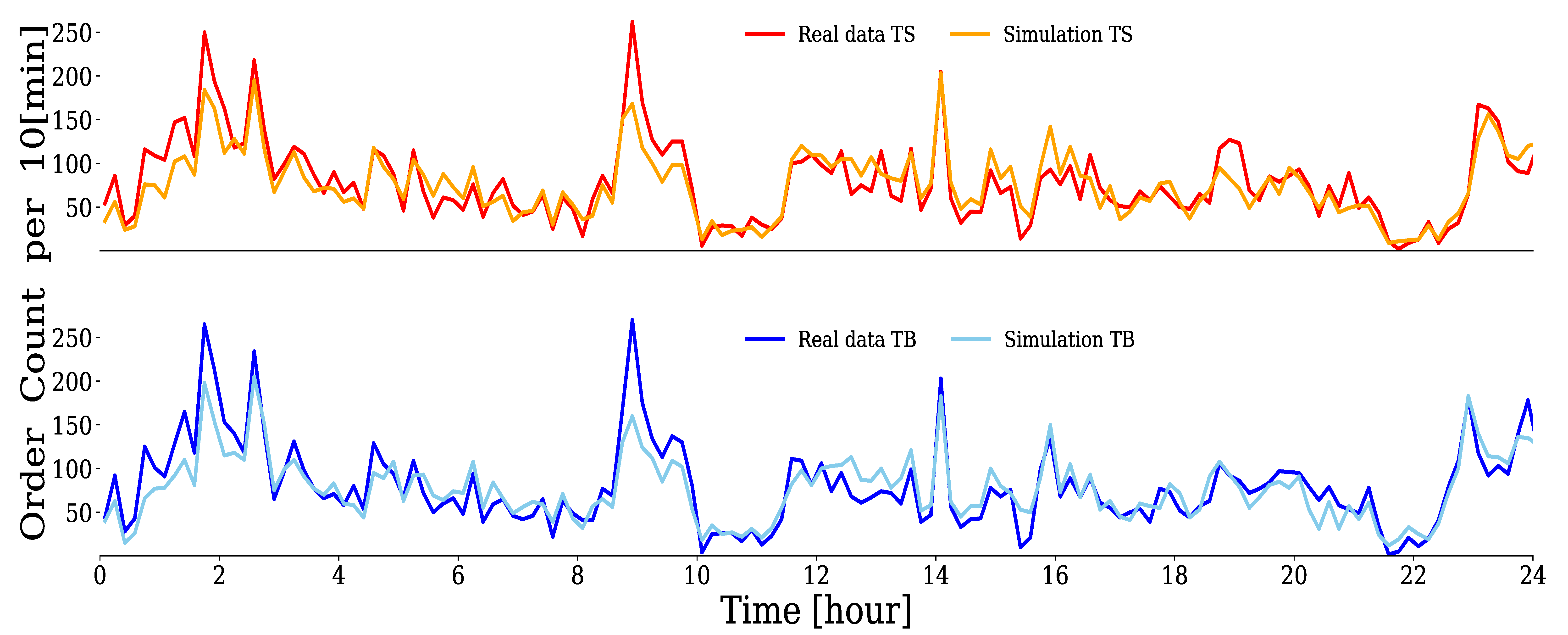
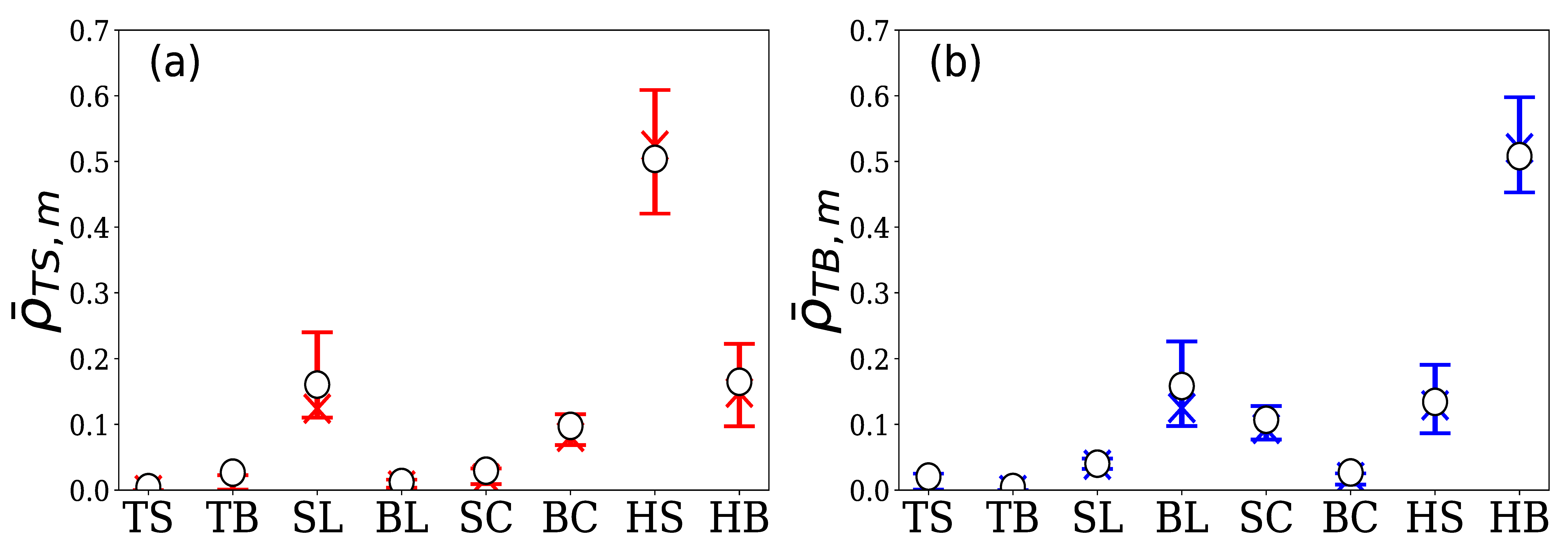
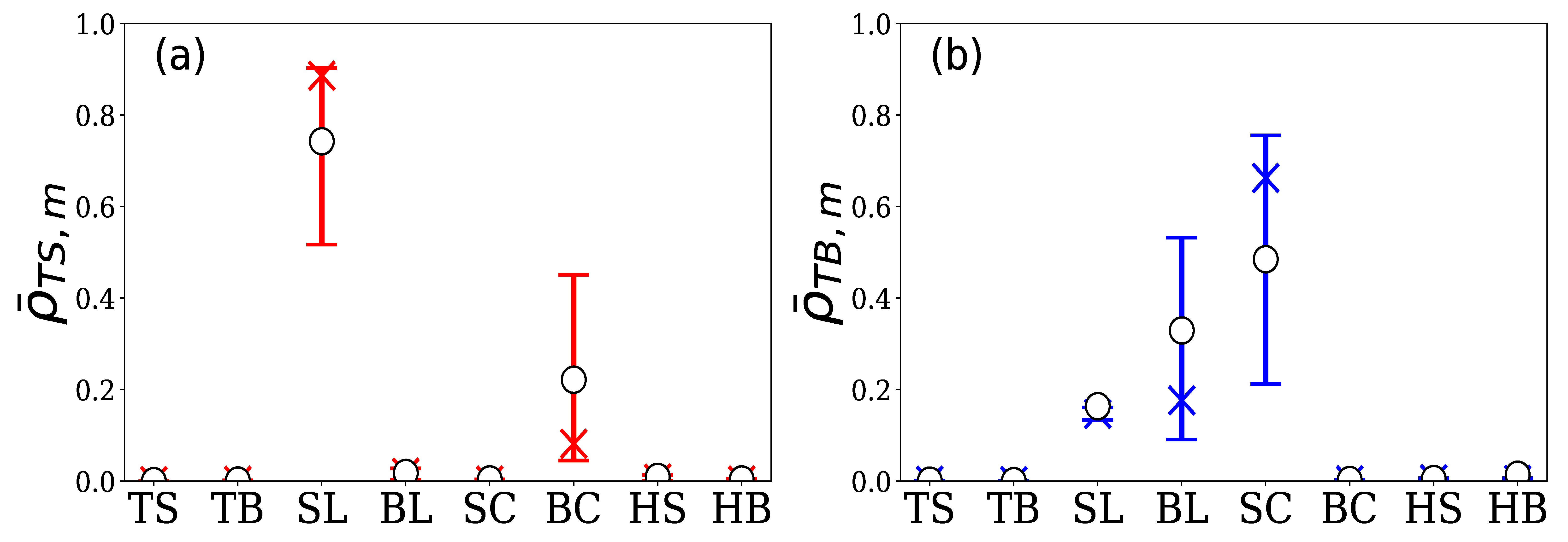
4.1. Calculation Results for All HFTs
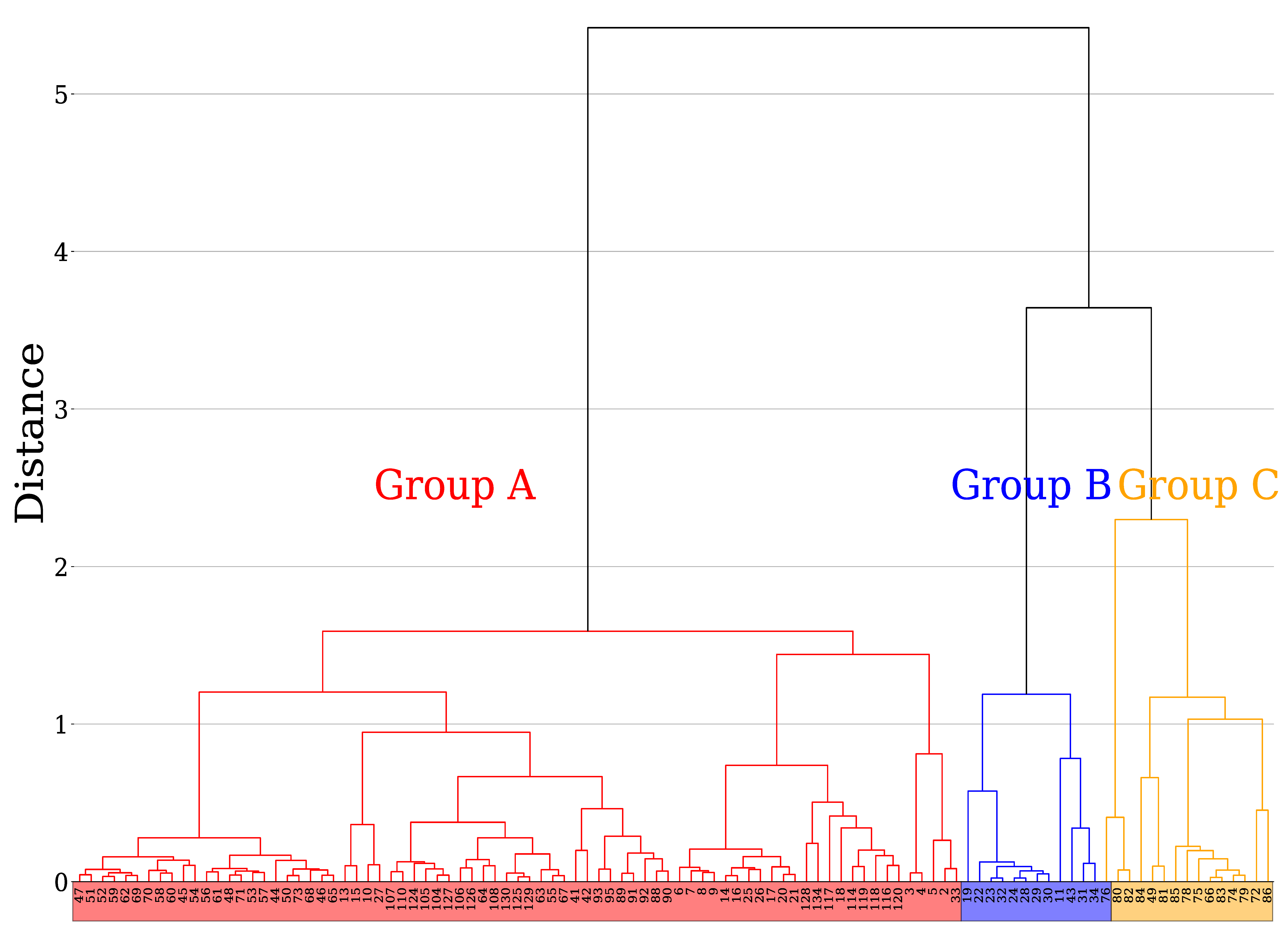
4.2. Results of Clustering Analysis
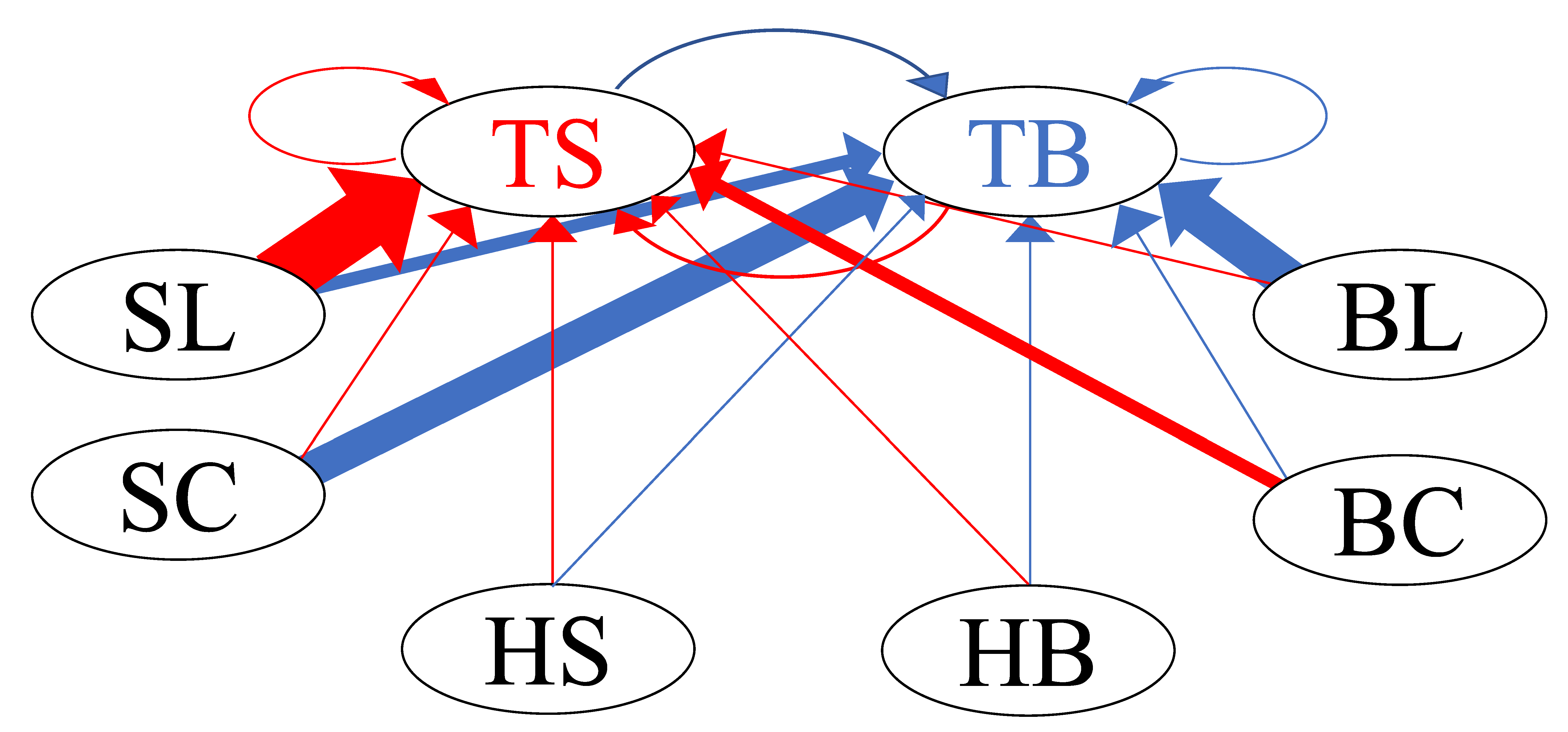
4.2.1. Group A
4.2.2. Group B
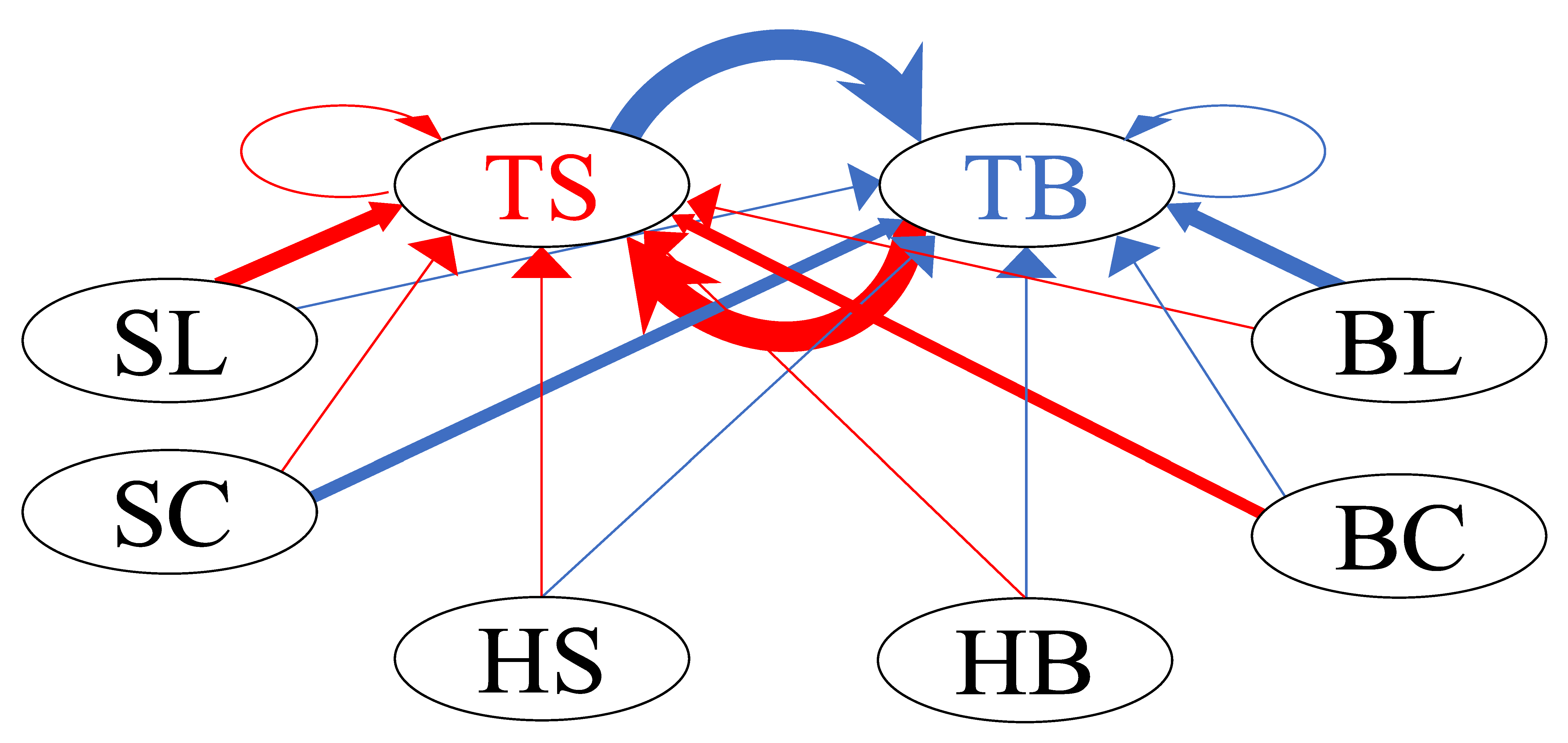
4.2.3. Group C
5. Conclusions
Author Contributions
Funding
Institutional Review Board Statement
Informed Consent Statement
Data Availability Statement
Acknowledgments
Conflicts of Interest
References
- Odean, T. Are investors reluctant to realize their losses? J. Financ. 1998, 53, 1775–1798. [Google Scholar] [CrossRef] [Green Version]
- Grinblatt, M.; Keloharju, M. The investment behavior and performance of various investor types: A study of Finland’s unique data set. J. Financ. Econ. 2000, 55, 43–67. [Google Scholar] [CrossRef]
- Sueshige, T.; Sornette, D.; Takayasu, H.; Takayasu, M. Classification of position management strategies at the order-book level and their influences on future market-price formation. PLoS ONE 2019, 14, e0220645. [Google Scholar] [CrossRef]
- Sueshige, T.; Kanazawa, K.; Takayasu, H.; Takayasu, M. Ecology of trading strategies in a forex market for limit and market orders. PLoS ONE 2018, 13, e0208332. [Google Scholar] [CrossRef] [PubMed]
- Kanazawa, K.; Sueshige, T.; Takayasu, H.; Takayasu, M. Kinetic theory for financial Brownian motion from microscopic dynamics. Phys. Rev. E 2018, 98, 052317. [Google Scholar] [CrossRef] [Green Version]
- Kanazawa, K.; Sueshige, T.; Takayasu, H.; Takayasu, M. Derivation of the Boltzmann equation for financial Brownian motion: Direct observation of the collective motion of high-frequency traders. Phys. Rev. Lett. 2018, 120, 138301. [Google Scholar] [CrossRef] [PubMed] [Green Version]
- Biais, B.; Foucault, T.; Moinas, S. Equilibrium fast trading. J. Financ. Econ. 2015, 116, 292–313. [Google Scholar] [CrossRef] [Green Version]
- Carrion, A. Very fast money: High-frequency trading on the NASDAQ. J. Financ. Mark. 2013, 16, 680–711. [Google Scholar] [CrossRef]
- Schmidt, A.B. Ecology of the Modern Institutional Spot FX: The EBS Market in 2011. 2012. Available online: https://papers.ssrn.com/sol3/papers.cfm?abstract_id=1984070 (accessed on 7 January 2022).
- Gerig, A. High-Frequency Trading Synchronizes Prices in Financial Markets. 2015. Available online: https://papers.ssrn.com/sol3/papers.cfm?abstract_id=2173247 (accessed on 7 January 2022).
- Mukerji, P.; Chung, C.; Walsh, T. The impact of algorithmic trading in a simulated asset market. J. Risk Financ. Manag. 2019, 12, 68. [Google Scholar] [CrossRef] [Green Version]
- O’Hara, M. High frequency market microstructure. J. Financ. Econ. 2015, 116, 257–270. [Google Scholar] [CrossRef]
- Goldstein, M.A.; Kumar, P.; Graves, F.C. Computerized and high-frequency trading. Financ. Rev. 2014, 49, 177–202. [Google Scholar] [CrossRef] [Green Version]
- Jones, C.M. What Do We Know about High-Frequency Trading? Columbia Business School Research Paper 13-11. 2013. Available online: https://papers.ssrn.com/sol3/papers.cfm?abstract_id=2236201 (accessed on 7 January 2022).
- Menkveld, A.J. High frequency trading and the new market makers. J. Financ. Mark. 2013, 16, 712–740. [Google Scholar] [CrossRef] [Green Version]
- Easley, D.; De Prado, M.M.L.; O’Hara, M. The microstructure of the “flash crash”: Flow toxicity, liquidity crashes, and the probability of informed trading. J. Portf. Manag. 2011, 37, 118–128. [Google Scholar] [CrossRef] [Green Version]
- Easley, D.; de Prado, M.M.L.; O’Hara, M. VPIN and the flash crash: A rejoinder. J. Financ. Mark. 2014, 17, 47–52. [Google Scholar] [CrossRef]
- Andersen, T.G.; Bondarenko, O. VPIN and the flash crash. J. Financ. Mark. 2014, 17, 1–46. [Google Scholar] [CrossRef]
- Andersen, T.G.; Bondarenko, O. Reflecting on the VPIN dispute. J. Financ. Mark. 2014, 17, 53–64. [Google Scholar] [CrossRef]
- Andersen, T.G.; Bondarenko, O. Assessing measures of order flow toxicity and early warning signals for market turbulence. Rev. Financ. 2015, 19, 1–54. [Google Scholar] [CrossRef]
- D’Souza, C. Where Does Price Discovery Occur in FX Markets? 2007. Available online: https://papers.ssrn.com/sol3/papers.cfm?abstract_id=966446 (accessed on 7 January 2022).
- Gençay, R.; Gradojevic, N.; Olsen, R.; Selçuk, F. Informed traders’ arrival in foreign exchange markets: Does geography matter? Empir. Econ. 2015, 49, 1431–1462. [Google Scholar] [CrossRef] [Green Version]
- Gençay, R.; Gradojevic, N. Private information and its origins in an electronic foreign exchange market. Econ. Model. 2013, 33, 86–93. [Google Scholar] [CrossRef]
- Gradojevic, N.; Erdemlioglu, D.; Gençay, R. Informativeness of trade size in foreign exchange markets. Econ. Lett. 2017, 150, 27–33. [Google Scholar] [CrossRef]
- Elaut, G.; Frömmel, M.; Lampaert, K. Intraday momentum in FX markets: Disentangling informed trading from liquidity provision. J. Financ. Mark. 2018, 37, 35–51. [Google Scholar] [CrossRef]
- Hawkes, A.G. Spectra of some self-exciting and mutually exciting point processes. Biometrika 1971, 58, 83–90. [Google Scholar] [CrossRef]
- Engle, R.F.; Russell, J.R. Forecasting the frequency of changes in quoted foreign exchange prices with the autoregressive conditional duration model. J. Empir. Financ. 1997, 4, 187–212. [Google Scholar] [CrossRef]
- Takayasu, M.; Takayasu, H. Self-modulation processes and resulting generic 1/f fluctuations. Phys. A Stat. Mech. Its Appl. 2003, 324, 101–107. [Google Scholar] [CrossRef]
- Hawkes, A.G. Hawkes processes and their applications to finance: A review. Quant. Financ. 2018, 18, 193–198. [Google Scholar] [CrossRef]
- Bowsher, C. Modelling security market events in continuous time: Intensity based, multivariate point process models. J. Econom. 2007, 141, 876–912. [Google Scholar] [CrossRef] [Green Version]
- Filimonov, V.; Sornette, D. Quantifying reflexivity in financial markets: Toward a prediction of flash crashes. Phys. Rev. E 2012, 85, 056108. [Google Scholar] [CrossRef] [Green Version]
- Hardiman, S.J.; Bercot, N.; Bouchaud, J.P. Critical reflexivity in financial markets: A Hawkes process analysis. Eur. Phys. J. B 2013, 86, 442. [Google Scholar] [CrossRef] [Green Version]
- Hardiman, S.J.; Bouchaud, J.P. Branching-ratio approximation for the self-exciting Hawkes process. Phys. Rev. E 2014, 90, 062807. [Google Scholar] [CrossRef] [Green Version]
- Bacry, E.; Muzy, J.F. First- and Second-Order Statistics Characterization of Hawkes Processes and Non-Parametric Estimation. IEEE Trans. Inf. Theory 2016, 62, 2184–2202. [Google Scholar] [CrossRef]
- Bacry, E.; Jaisson, T.; Muzy, J.F. Estimation of slowly decreasing hawkes kernels: Application to high-frequency order book dynamics. Quant. Financ. 2016, 16, 1179–1201. [Google Scholar] [CrossRef]
- Achab, M.; Bacry, E.; Muzy, J.F.; Rambaldi, M. Analysis of order book flows using a non-parametric estimation of the branching ratio matrix. Quant. Financ. 2018, 18, 199–212. [Google Scholar] [CrossRef] [Green Version]
- Rambaldi, M.; Pennesi, P.; Lillo, F. Modeling foreign exchange market activity around macroeconomic news: Hawkes-process approach. Phys. Rev. E 2015, 91, 012819. [Google Scholar] [CrossRef] [PubMed] [Green Version]
- Rambaldi, M.; Bacry, E.; Lillo, F. The role of volume in order book dynamics: A multivariate Hawkes process analysis. Quant. Financ. 2017, 17, 999–1020. [Google Scholar] [CrossRef]
- Rambaldi, M.; Filimonov, V.; Lillo, F. Detection of intensity bursts using Hawkes processes: An application to high-frequency financial data. Phys. Rev. E 2018, 97, 032318. [Google Scholar] [CrossRef] [PubMed] [Green Version]
- Lu, X.; Abergel, F. High-dimensional Hawkes processes for limit order books: Modelling, empirical analysis and numerical calibration. Quant. Financ. 2018, 18, 249–264. [Google Scholar] [CrossRef] [Green Version]
- Fosset, A.; Bouchaud, J.P.; Benzaquen, M. Non-parametric estimation of quadratic Hawkes processes for order book events. Eur. J. Financ. 2021. [Google Scholar] [CrossRef]
- Rizoiu, M.A.; Lee, Y.; Mishra, S.; Xie, L. A tutorial on hawkes processes for events in social media. arXiv 2017, arXiv:1708.06401. [Google Scholar]
- Hawkes, A.G. Point Spectra of Some Mutually Exciting Point Processes. J. R. Stat. Soc. Ser. B Methodol. 1971, 33, 438–443. [Google Scholar] [CrossRef]
- Bacry, E.; Mastromatteo, I.; Muzy, J.F. Hawkes processes in finance. Mark. Microstruct. Liq. 2015, 1, 1550005. [Google Scholar] [CrossRef]
- Helmstetter, A.; Sornette, D. Importance of direct and indirect triggered seismicity in the ETAS model of seismicity. Geophys. Res. Lett. 2003, 30. [Google Scholar] [CrossRef] [Green Version]
- Helmstetter, A.; Sornette, D. Subcritical and supercritical regimes in epidemic models of earthquake aftershocks. J. Geophys. Res. Solid Earth 2002, 107, ESE-10. [Google Scholar] [CrossRef]
- Toke, I.M. An Introduction to Hawkes Processes with Applications to Finance. Lectures Notes from Ecole Centrale Paris, BNP Paribas Chair of Quantitative Finance. 2011, Volume 193. Available online: http://www.smallake.kr/wp-content/uploads/2015/01/HawkesCourseSlides.pdf (accessed on 7 January 2022).
- Kingma, D.P.; Ba, J. Adam: A method for stochastic optimization. arXiv 2014, arXiv:1412.6980. [Google Scholar]
- Ogata, Y. On Lewis’ simulation method for point processes. IEEE Trans. Inf. Theory 1981, 27, 23–31. [Google Scholar] [CrossRef] [Green Version]
- Ogata, Y. Statistical models for earthquake occurrences and residual analysis for point processes. J. Am. Stat. Assoc. 1988, 83, 9–27. [Google Scholar] [CrossRef]
- Lewis, P.W.; Shedler, G.S. Simulation of nonhomogeneous Poisson processes by thinning. Nav. Res. Logist. Q. 1979, 26, 403–413. [Google Scholar] [CrossRef]
- Ward, J.H., Jr. Hierarchical grouping to optimize an objective function. J. Am. Stat. Assoc. 1963, 58, 236–244. [Google Scholar] [CrossRef]


| Date | Order Time | Trader ID | Order Type | USD/JPY | Volume | Deal Time |
|---|---|---|---|---|---|---|
| 5 June 2016 | 21:00:12.946 | 578 | Sell limit | 106.515 | 1 | – |
| 5 June 2016 | 21:01:13.647 | HT6 | Buy cancel | 105.390 | 2 | – |
| 5 June 2016 | 21:02:20.148 | JR1 | Buy limit | 105.405 | 1 | 21:02:20.499 |
| 5 June 2016 | 21:02:20.499 | HSH | Sell market | 105.405 | 1 | 21:02:20.499 |
| 5 June 2016 | 21:03:00.950 | 7KP | Bid market | 106.470 | 1 | – |
| ⋮ | ⋮ | ⋮ | ⋮ | ⋮ | ⋮ | ⋮ |
| 10 June 2016 | 20:59:20.148 | HT6 | Buy Limit | 107.405 | 3 | 20:59:29.072 |
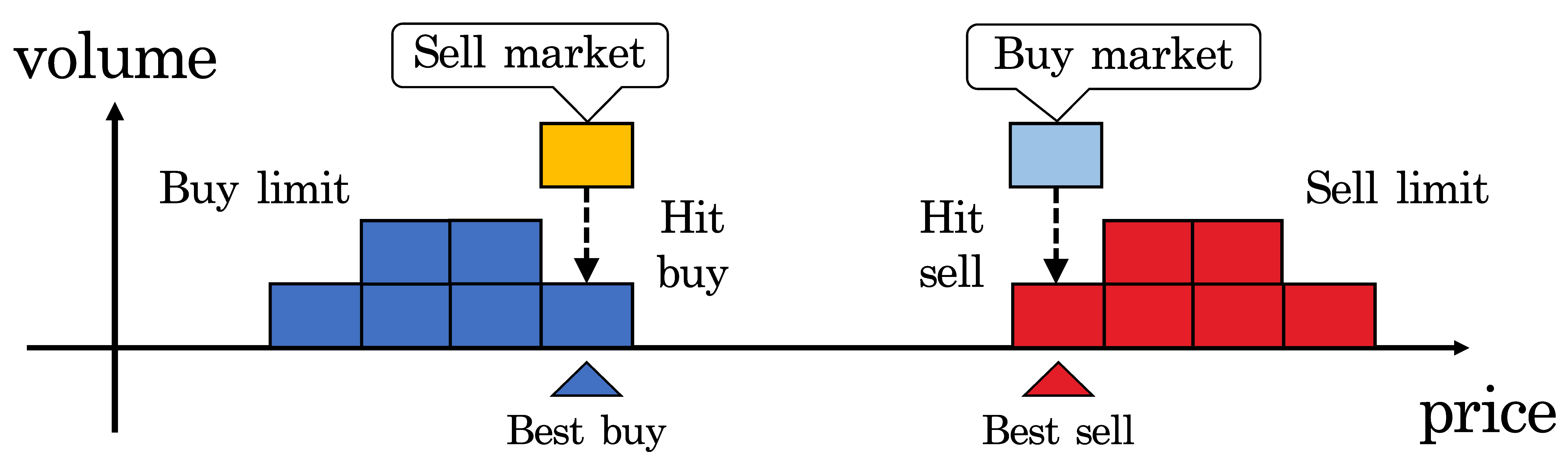
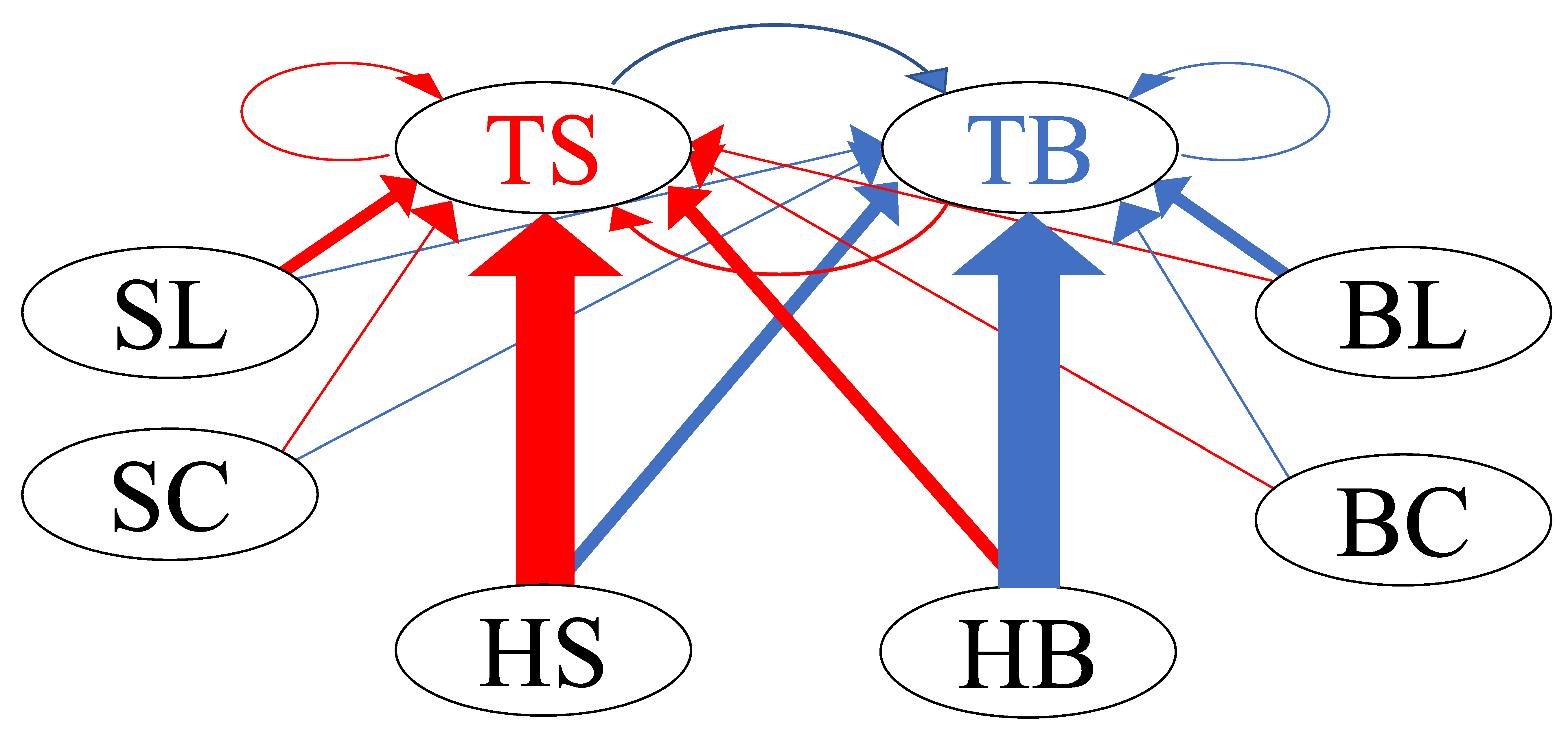
| TS | : | Sell limit of the target HFT itself | TB | : | Buy limit of the target HFT itself |
| SL | : | Sell limit in order book | BL | : | Buy limit in order book |
| SC | : | Sell cancel in order book | BC | : | Buy cancel in order book |
| HS | : | Hit sell | HB | : | Hit buy |
| m | TS | TB | SL | BL | SC | BC | HS | HB | |
|---|---|---|---|---|---|---|---|---|---|
| n | |||||||||
| TS | 0.102 | 0.295 | 0.076 | 0.087 | 0.081 | 0.069 | 0.110 | 0.404 | |
| TB | 0.118 | 0.099 | 0.114 | 0.071 | 0.066 | 0.091 | 0.148 | 0.111 | |
| m | TS | TB | SL | BL | SC | BC | HS | HB | |
|---|---|---|---|---|---|---|---|---|---|
| n | |||||||||
| TS | 0.099 | 0.100 | 0.681 | 0.109 | 0.110 | 0.285 | 0.101 | 0.099 | |
| TB | 0.099 | 0.100 | 0.259 | 0.373 | 0.558 | 0.105 | 0.099 | 0.101 | |
| m | TS | TB | SL | BL | SC | BC | HS | HB | |
|---|---|---|---|---|---|---|---|---|---|
| n | |||||||||
| TS | 0.134 | 17.781 | 0.266 | 0.099 | 0.096 | 0.359 | 0.109 | 0.154 | |
| TB | 11.201 | 0.098 | 0.269 | 0.258 | 0.355 | 0.094 | 0.132 | 0.103 | |
Publisher’s Note: MDPI stays neutral with regard to jurisdictional claims in published maps and institutional affiliations. |
© 2022 by the authors. Licensee MDPI, Basel, Switzerland. This article is an open access article distributed under the terms and conditions of the Creative Commons Attribution (CC BY) license (https://creativecommons.org/licenses/by/4.0/).
Share and Cite
Watari, H.; Takayasu, H.; Takayasu, M. Analysis of Individual High-Frequency Traders’ Buy–Sell Order Strategy Based on Multivariate Hawkes Process. Entropy 2022, 24, 214. https://doi.org/10.3390/e24020214
Watari H, Takayasu H, Takayasu M. Analysis of Individual High-Frequency Traders’ Buy–Sell Order Strategy Based on Multivariate Hawkes Process. Entropy. 2022; 24(2):214. https://doi.org/10.3390/e24020214
Chicago/Turabian StyleWatari, Hiroki, Hideki Takayasu, and Misako Takayasu. 2022. "Analysis of Individual High-Frequency Traders’ Buy–Sell Order Strategy Based on Multivariate Hawkes Process" Entropy 24, no. 2: 214. https://doi.org/10.3390/e24020214
APA StyleWatari, H., Takayasu, H., & Takayasu, M. (2022). Analysis of Individual High-Frequency Traders’ Buy–Sell Order Strategy Based on Multivariate Hawkes Process. Entropy, 24(2), 214. https://doi.org/10.3390/e24020214