Author Contributions
Conceptualization, S.J.M. and D.O.; Formal analysis, S.J.M. and D.Z.; Investigation, S.J.M.; Methodology, S.J.M., D.O., M.P.-C. and G.S.; Software, S.J.M. and D.Z.; Supervision, S.J.M., D.O.; Validation, S.J.M., D.Z. and G.S.; Visualization, S.J.M.; Writing—original draft, S.J.M.; Writing—review & editing, D.O., M.P.-C. and G.S. All authors have read and agreed to the published version of the manuscript.
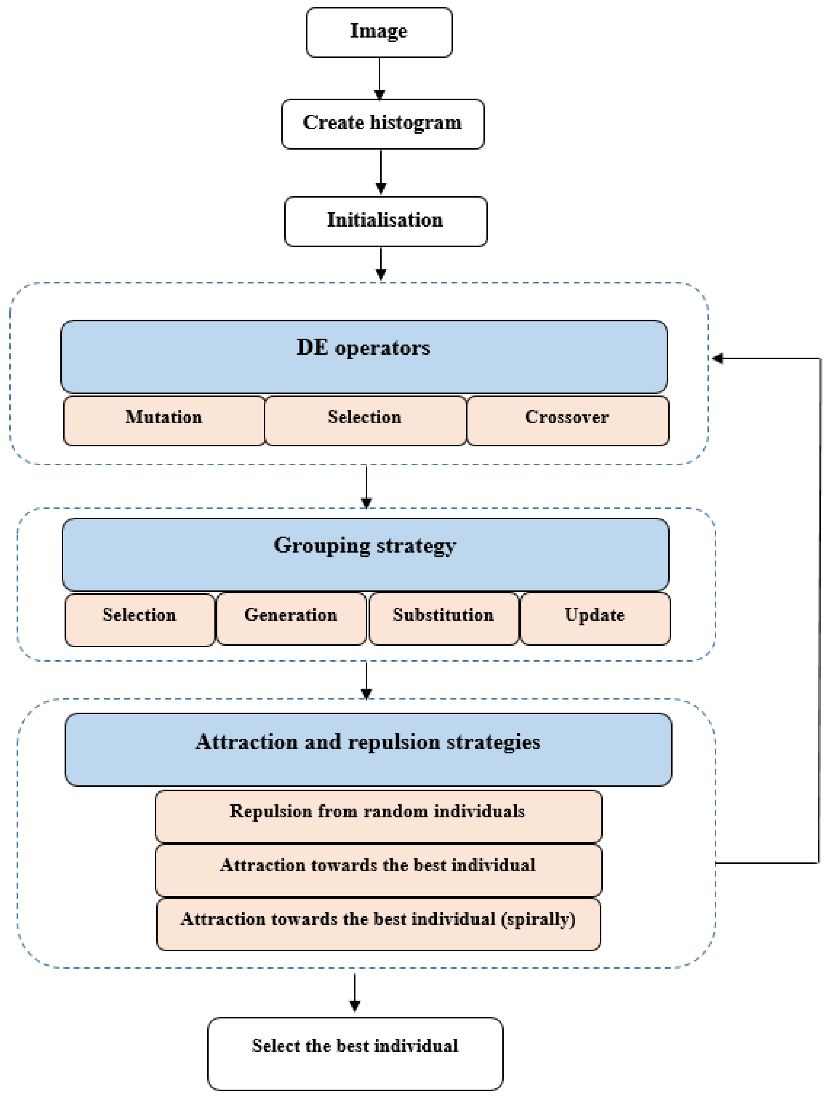
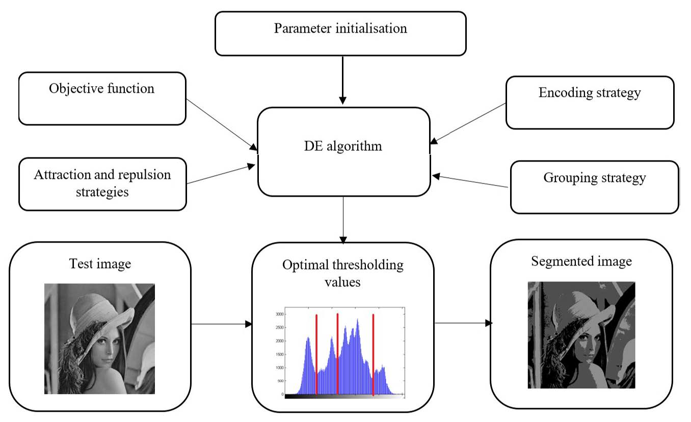
Figure 1.
General structure of the ME-GDEAR algorithm.
Figure 1.
General structure of the ME-GDEAR algorithm.
Figure 2.
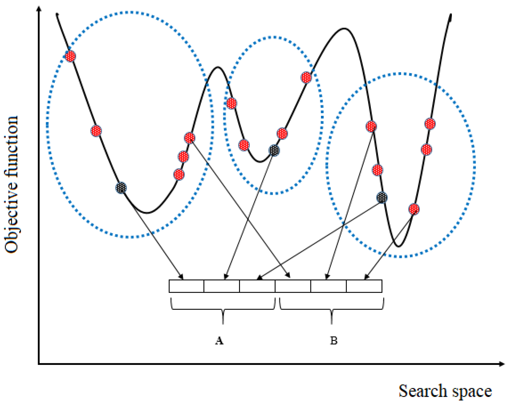
Population clustering: red points represent individuals and black points indicate cluster centres. The population is divided into 3 clusters. A is the set of cluster centres while B contains some random individuals.
Figure 2.
Population clustering: red points represent individuals and black points indicate cluster centres. The population is divided into 3 clusters. A is the set of cluster centres while B contains some random individuals.
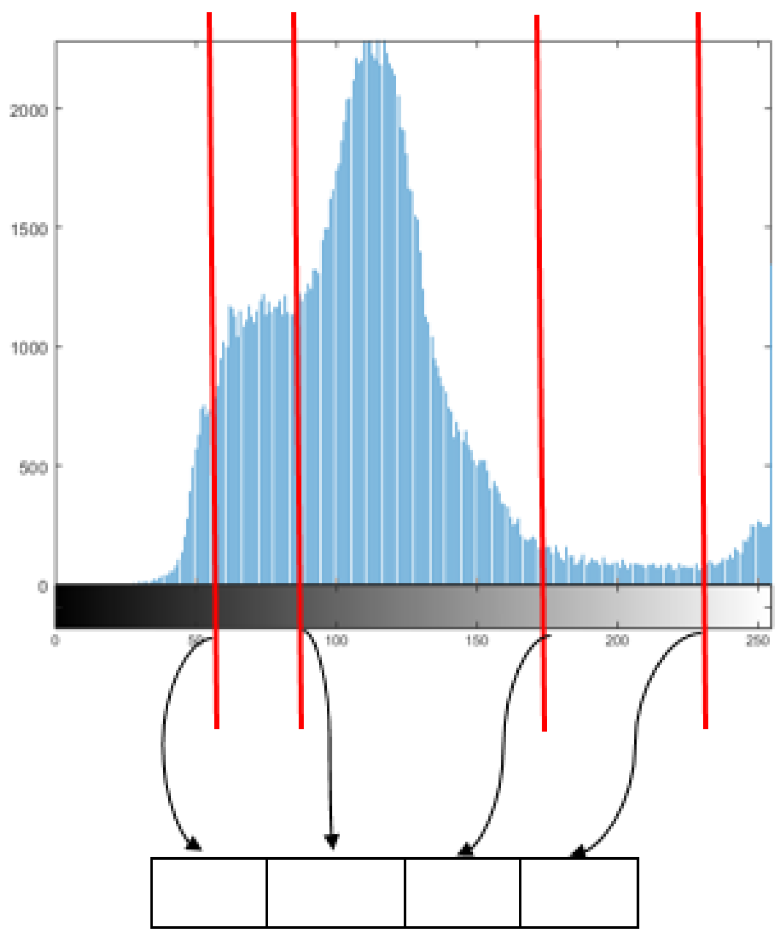
Figure 3.
Encoding strategy in ME-GDEAR.
Figure 3.
Encoding strategy in ME-GDEAR.
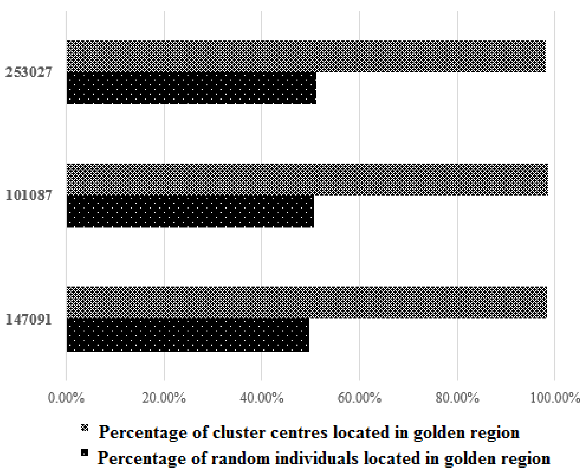
Figure 4.
Fractions of cluster centres and random individuals located in the golden region.
Figure 4.
Fractions of cluster centres and random individuals located in the golden region.
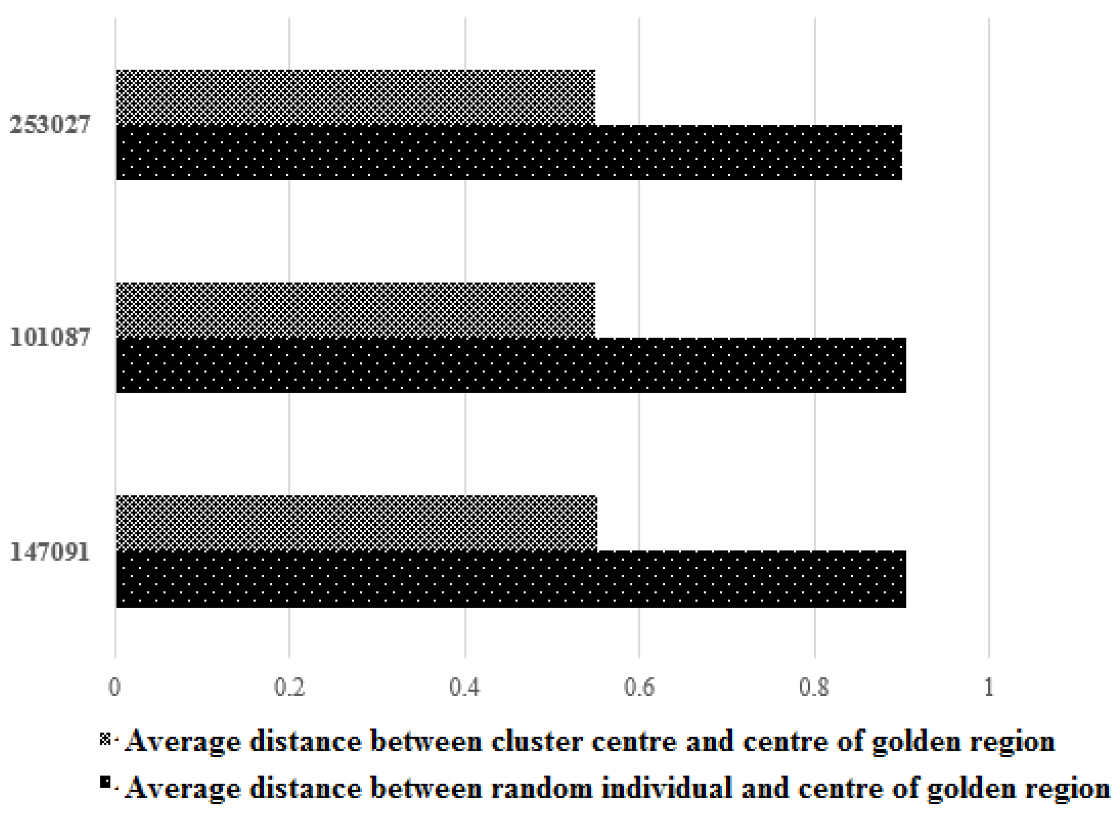
Figure 5.
Distance between the centre of the golden region and the cluster centres/random individuals.
Figure 5.
Distance between the centre of the golden region and the cluster centres/random individuals.
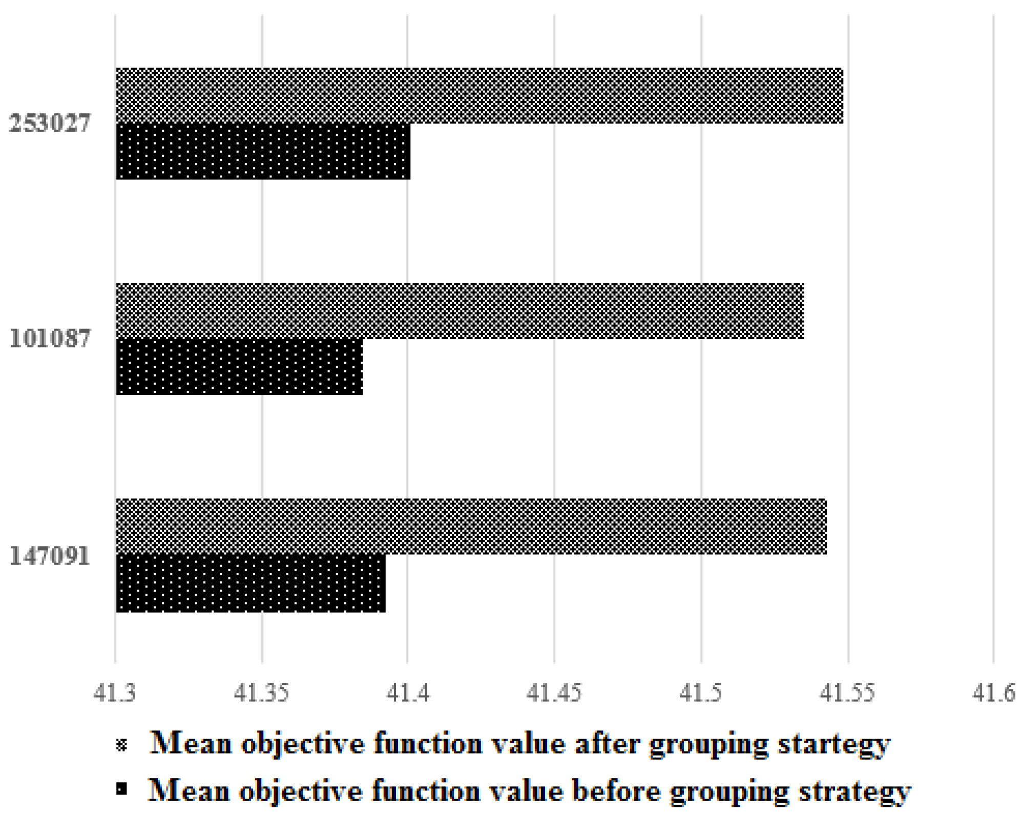
Figure 6.
Mean objective function results with/without grouping strategy.
Figure 6.
Mean objective function results with/without grouping strategy.
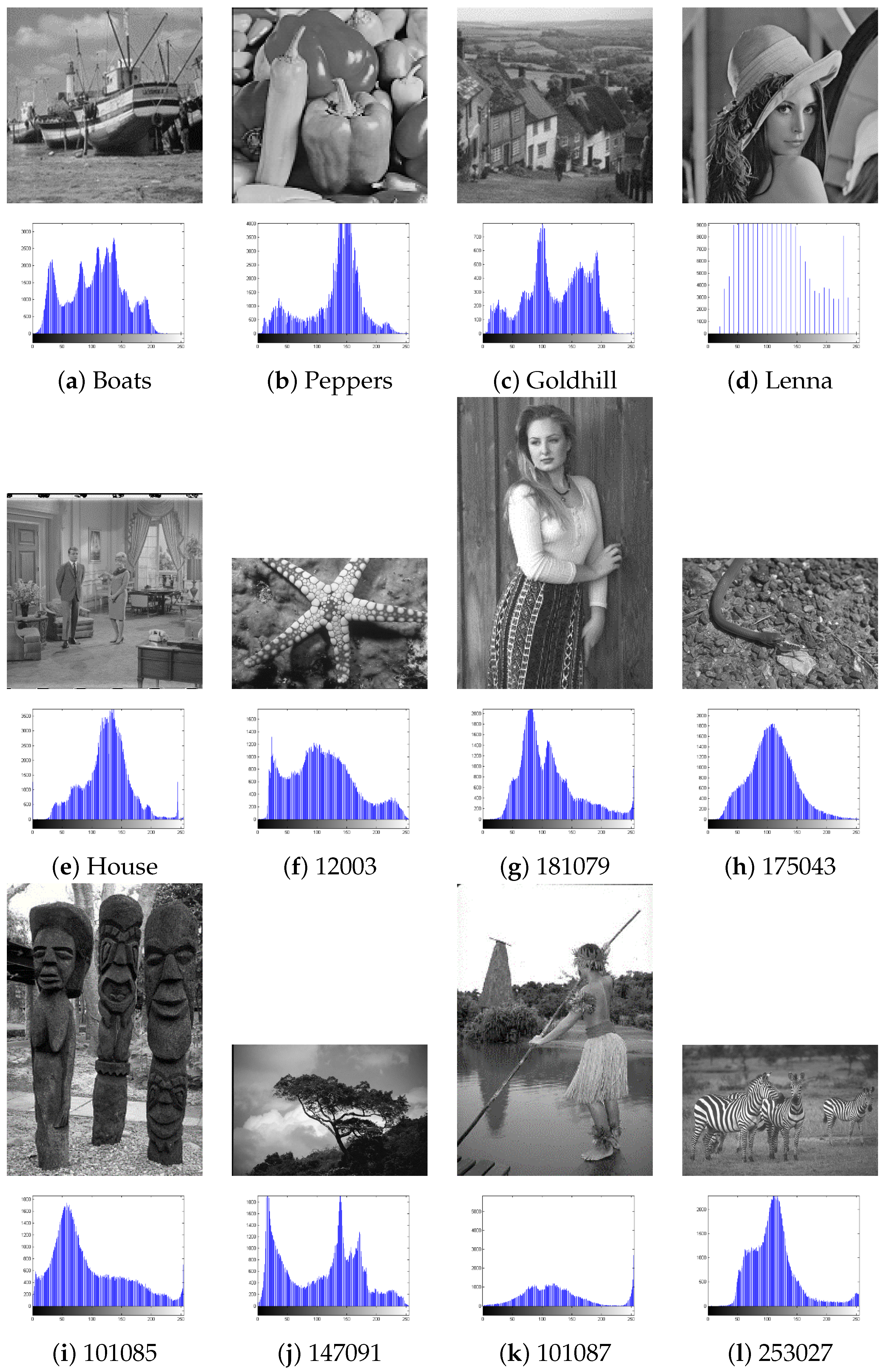
Figure 7.
Test images and their histograms.
Figure 7.
Test images and their histograms.
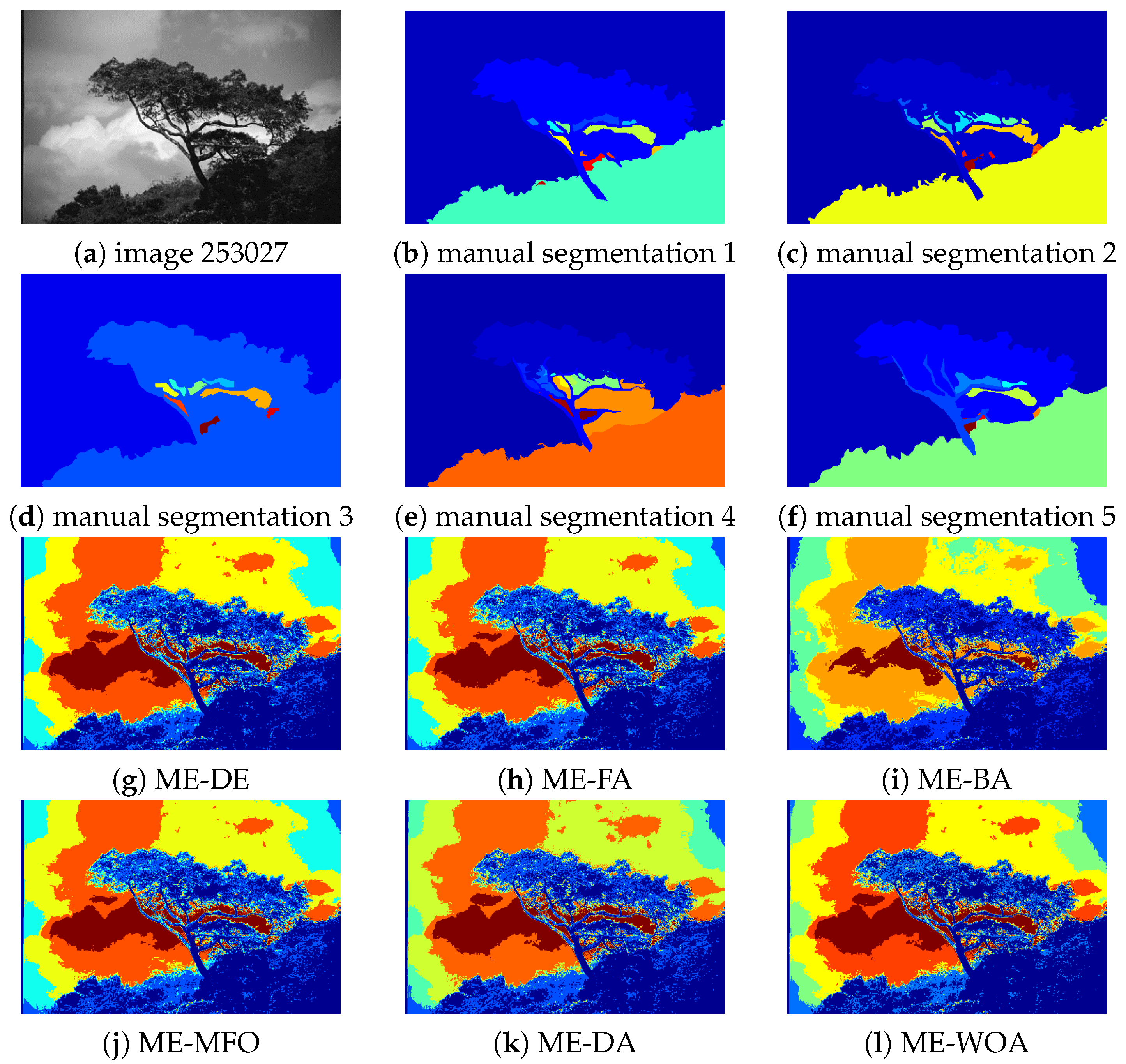
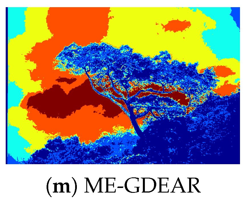
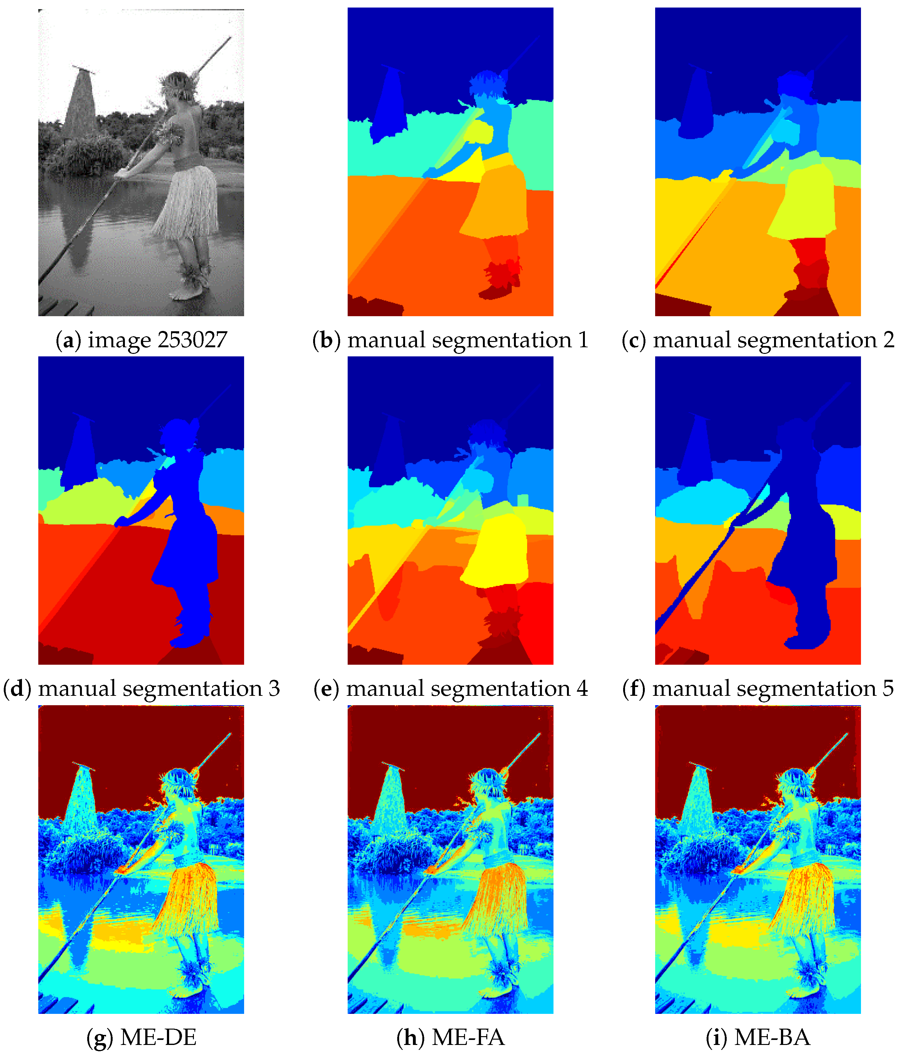
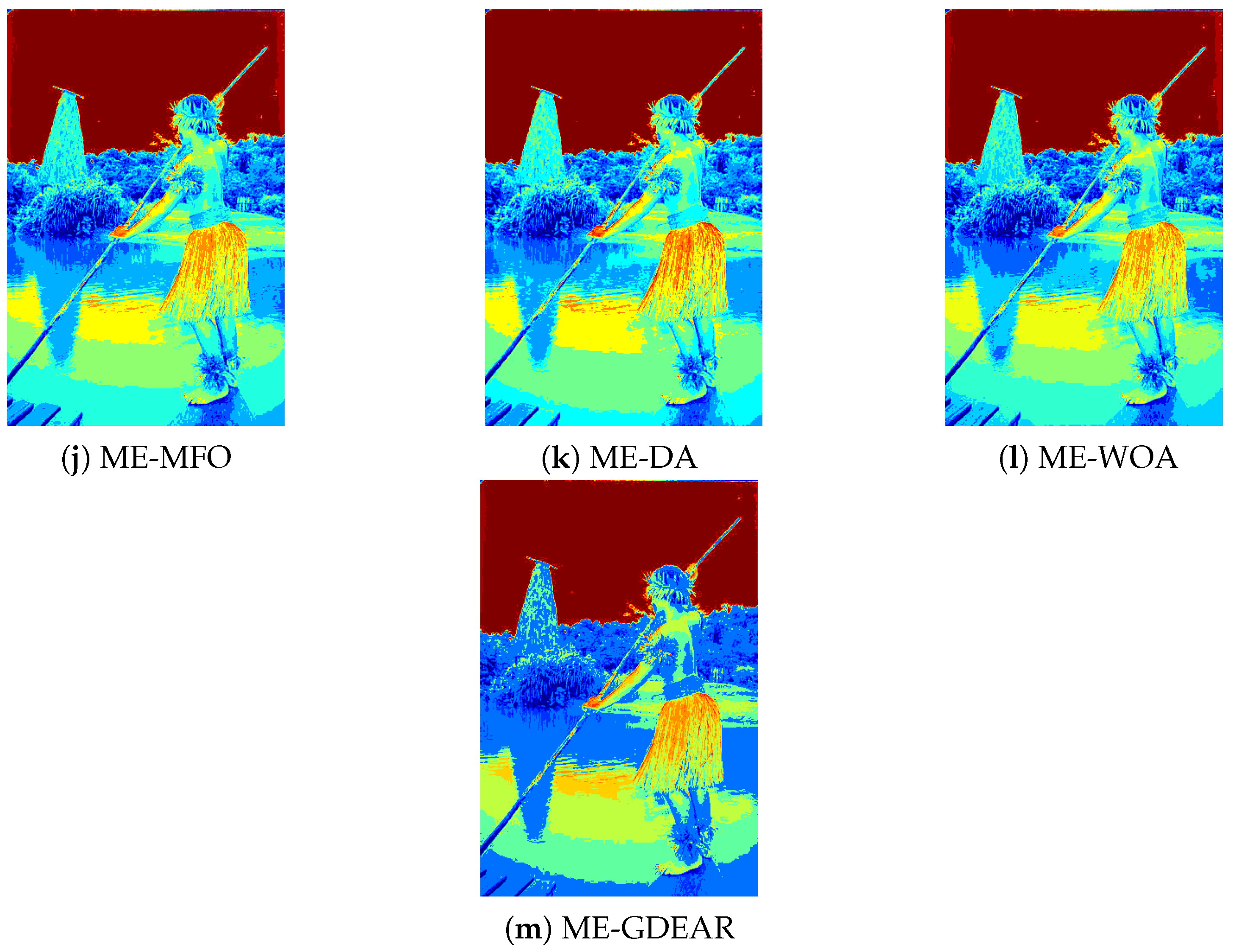
Figure 8.
Thresholding results for image 147091 for . (a) Original image, (b–f) true manual segmentation, (g) segmented image for ME-DE, (h) segmented image for ME-FA, (i) segmented image for ME-BA, (j) segmented image for ME-MFO, (k) segmented image ME-DA, (l) segmented image for ME-WOA, and (m) segmented image for ME-GDEAR.
Figure 9.
Thresholding results for image 101087 for . (a): original image, (b–f): different manual segmentations, (g) segmented image for ME-DE, (h) segmented image for ME-FA,(i) segmented image for ME-BA, (j) segmented image for ME-MFO, (k) segmented image for ME-DA, (l) segmented image for ME-WOA, and (m) segmented image for ME-GDEAR.
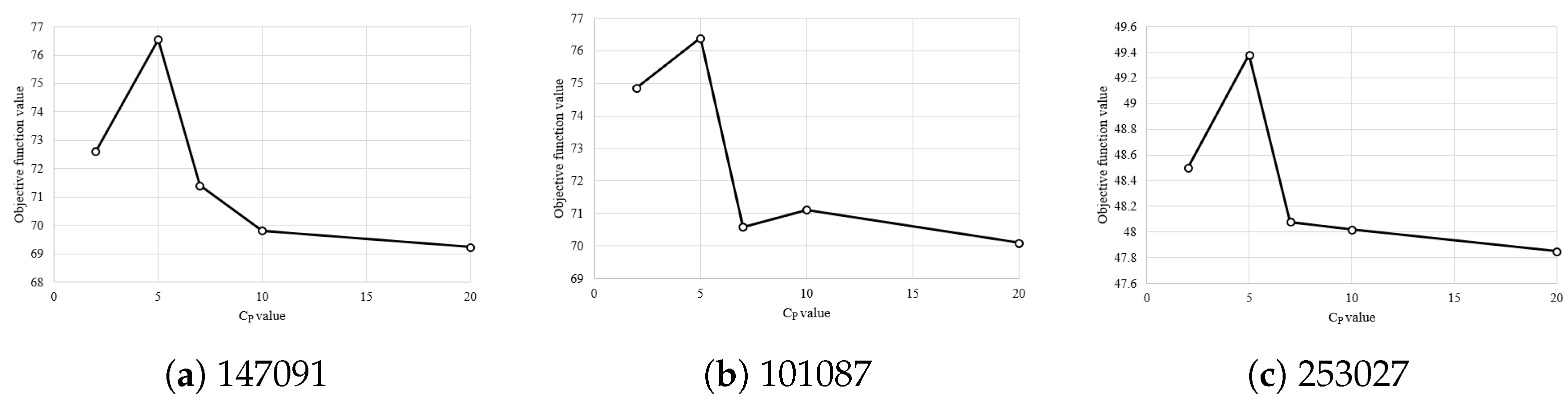
Figure 10.
Effect of on the mean objective function value for images (a) 147091, (b) 101087, and (c) 253027 for .
Figure 10.
Effect of on the mean objective function value for images (a) 147091, (b) 101087, and (c) 253027 for .
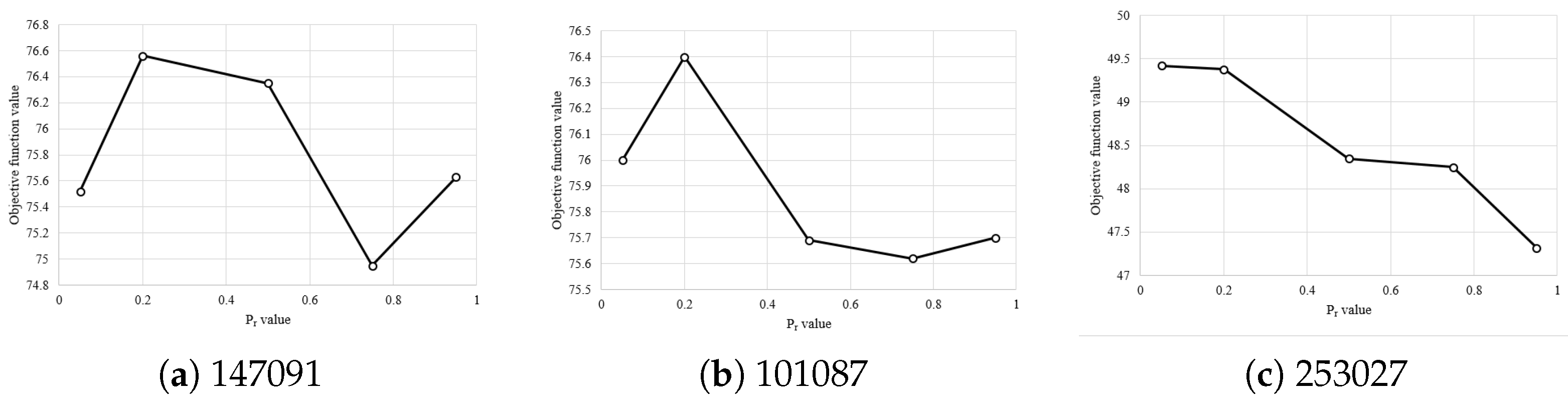
Figure 11.
Effect of on the mean objective function value for images (a) 147091, (b) 101087, and (c) 253027 for .
Figure 11.
Effect of on the mean objective function value for images (a) 147091, (b) 101087, and (c) 253027 for .
Table 1.
Parameter settings for the experiments.
Table 1.
Parameter settings for the experiments.
| Algorithm | Parameter | Value |
|---|
| ME-DE [33] | scaling factor | 0.5 |
| | crossover probability | 0.9 |
| ME-FA [49] | light absorption coefficient () | 1 |
| | attractiveness at () | 1 |
| | scaling factor | 0.25 |
| ME-BA [50] | loudness | 0.5 |
| | pulse rate | 0.5 |
| ME-MFO [51] | a | −1 |
| | b | 1 |
| ME-DA [52] | no parameters | |
| ME-WOA [46] | constant defining shape of logarithmic spiral | 1 |
| ME-GDEAR | scaling factor | 0.5 |
| | crossover probability | 0.9 |
| | clustering period | 0.5 |
| | | 0.2 |
Table 2.
Objective function results for .
Table 2.
Objective function results for .
| Image | | ME-DE | ME-FA | ME-BA | ME-MFO | ME-DA | ME-WOA | ME-GDEAR |
|---|
| Boats | mean | 35.23 | 34.25 | 33.98 | 34.85 | 34.73 | 34.45 | 34.71 |
| | std.dev. | 0.02 | 0.97 | 0.96 | 0.49 | 0.54 | 0.41 | 0.64 |
| | rank | 1 | 6 | 7 | 2 | 3 | 5 | 4 |
| Peppers | mean | 66.20 | 63.92 | 58.27 | 64.23 | 66.42 | 61.71 | 66.33 |
| | std.dev. | 8.75 | 9.26 | 7.95 | 6.94 | 7.98 | 10.34 | 6.51 |
| | rank | 3 | 5 | 7 | 4 | 1 | 6 | 2 |
| Goldhill | mean | 15.56 | 15.77 | 15.28 | 16.03 | 15.76 | 15.42 | 16.05 |
| | std.dev. | 0.21 | 0.57 | 0.93 | 0.12 | 0.31 | 0.89 | 0.03 |
| | rank | 5 | 3 | 7 | 2 | 4 | 6 | 1 |
| Lenna | mean | 70.74 | 64.87 | 62.04 | 65.91 | 61.05 | 63.54 | 67.10 |
| | std.dev. | 2.17 | 5.39 | 5.83 | 5.67 | 4.92 | 6.56 | 5.04 |
| | rank | 1 | 4 | 6 | 3 | 7 | 5 | 2 |
| House | mean | 64.75 | 66.38 | 64.67 | 64.43 | 64.69 | 65.16 | 66.64 |
| | std.dev. | 2.92 | 7.13 | 3.44 | 1.5cm7 | 4.10 | 7.84 | 4.36 |
| | rank | 4 | 2 | 6 | 7 | 5 | 3 | 1 |
| 12003 | mean | 66.30 | 62.38 | 58.57 | 62.06 | 64.88 | 64.44 | 64.29 |
| | std.dev. | 6.61 | 6.47 | 5.77 | 7.10 | 5.17 | 6.29 | 7.17 |
| | rank | 1 | 5 | 7 | 6 | 2 | 3 | 4 |
| 181079 | mean | 66.24 | 63.42 | 60.68 | 67.24 | 61.74 | 61.07 | 63.29 |
| | std.dev. | 3.44 | 7.56 | 5.97 | 3.94 | 5.25 | 7.62 | 6.61 |
| | rank | 2 | 3 | 7 | 1 | 5 | 6 | 4 |
| 175043 | mean | 63.16 | 65.59 | 59.16 | 63.62 | 62.32 | 61.72 | 64.77 |
| | std.dev. | 3.50 | 6.04 | 4.16 | 4.75 | 5.49 | 6.50 | 6.30 |
| | rank | 4 | 1 | 7 | 3 | 5 | 6 | 2 |
| 101085 | mean | 63.96 | 62.49 | 61.59 | 64.08 | 66.85 | 61.21 | 66.20 |
| | std.dev. | 4.86 | 5.71 | 5.09 | 5.41 | 3.05 | 5.94 | 5.69 |
| | rank | 4 | 5 | 6 | 3 | 1 | 7 | 2 |
| 147091 | mean | 67.88 | 67.97 | 65.16 | 67.62 | 66.95 | 65.15 | 68.05 |
| | std.dev. | 1.56 | 2.70 | 3.82 | 1.61 | 1.20 | 4.40 | 2.22 |
| | rank | 3 | 2 | 6 | 4 | 5 | 7 | 1 |
| 101087 | mean | 59.46 | 65.73 | 60.56 | 64.92 | 63.64 | 64.99 | 71.12 |
| | std.dev. | 7.20 | 9.02 | 7.60 | 7.09 | 7.42 | 8.55 | 3.91 |
| | rank | 7 | 2 | 6 | 4 | 5 | 3 | 1 |
| 253027 | mean | 29.99 | 30.07 | 29.87 | 30.03 | 29.92 | 29.97 | 30.03 |
| | std.dev. | 0.07 | 0.07 | 0.23 | 0.13 | 0.17 | 0.16 | 0.13 |
| | rank | 4 | 1 | 7 | 2 | 6 | 5 | 3 |
| average rank | 3.25 | 3.25 | 6.58 | 3.42 | 4.08 | 5.17 | 2.25 |
| overall rank | 2.5 | 2.5 | 7 | 4 | 5 | 6 | 1 |
Table 3.
Objective function results for .
Table 3.
Objective function results for .
| Image | | ME-DE | ME-FA | ME-BA | ME-MFO | ME-DA | ME-WOA | ME-GDEAR |
|---|
| Boats | mean | 35.39 | 35.84 | 35.22 | 35.87 | 35.79 | 35.80 | 35.84 |
| | std.dev. | 0.20 | 0.02 | 0.48 | 0.11 | 0.19 | 0.21 | 0.02 |
| | rank | 6 | 3 | 7 | 1 | 5 | 4 | 2 |
| Peppers | mean | 66.45 | 65.67 | 62.46 | 68.23 | 66.39 | 64.90 | 71.57 |
| | std.dev. | 6.49 | 10.13 | 8.86 | 7.65 | 7.90 | 9.98 | 7.94 |
| | rank | 3 | 5 | 7 | 2 | 4 | 6 | 1 |
| Goldhill | mean | 16.80 | 17.32 | 17.24 | 18.14 | 17.21 | 16.87 | 17.61 |
| | std.dev. | 0.47 | 0.29 | 0.56 | 0.42 | 0.31 | 0.75 | 0.35 |
| | rank | 7 | 3 | 4 | 1 | 5 | 6 | 2 |
| Lenna | mean | 71.57 | 66.49 | 63.34 | 68.87 | 63.74 | 65.17 | 70.22 |
| | std.dev. | 2.06 | 5.90 | 5.44 | 5.58 | 5.09 | 6.61 | 5.22 |
| | rank | 1 | 4 | 7 | 3 | 6 | 5 | 2 |
| House | mean | 64.92 | 67.11 | 64.48 | 67.14 | 65.55 | 64.82 | 68.62 |
| | std.dev. | 2.41 | 8.91 | 2.61 | 4.27 | 3.78 | 7.53 | 4.19 |
| | rank | 5 | 3 | 7 | 2 | 4 | 6 | 1 |
| 12003 | mean | 65.84 | 63.35 | 63.79 | 66.29 | 69.58 | 64.16 | 68.69 |
| | std.dev. | 7.14 | 7.49 | 6.69 | 6.40 | 3.66 | 7.12 | 5.71 |
| | rank | 4 | 7 | 6 | 3 | 1 | 5 | 2 |
| 181079 | mean | 68.29 | 68.97 | 60.33 | 68.33 | 65.18 | 62.18 | 65.78 |
| | std.dev. | 2.79 | 5.29 | 5.14 | 4.08 | 5.40 | 7.61 | 6.79 |
| | rank | 3 | 1 | 7 | 2 | 5 | 6 | 4 |
| 175043 | mean | 62.84 | 67.97 | 61.56 | 63.57 | 62.61 | 59.77 | 66.16 |
| | std.dev. | 3.63 | 5.65 | 4.35 | 3.52 | 5.77 | 6.05 | 6.07 |
| | rank | 4 | 1 | 6 | 3 | 5 | 7 | 2 |
| 101085 | mean | 64.24 | 64.36 | 62.44 | 66.87 | 69.09 | 65.96 | 68.04 |
| | std.dev. | 4.22 | 5.80 | 4.35 | 5.69 | 1.54 | 5.86 | 4.98 |
| | rank | 6 | 5 | 7 | 3 | 1 | 4 | 2 |
| 147091 | mean | 70.11 | 70.11 | 68.22 | 69.73 | 69.41 | 66.69 | 70.68 |
| | std.dev. | 2.28 | 3.40 | 4.16 | 1.88 | 1.64 | 5.46 | 2.28 |
| | rank | 2 | 3 | 6 | 4 | 5 | 7 | 1 |
| 101087 | mean | 62.25 | 69.13 | 62.67 | 68.57 | 69.01 | 66.49 | 70.57 |
| | std.dev. | 5.94 | 10.06 | 6.96 | 7.21 | 8.01 | 9.04 | 7.82 |
| | rank | 7 | 2 | 6 | 4 | 3 | 5 | 1 |
| 253027 | mean | 32.99 | 33.22 | 32.89 | 33.26 | 33.18 | 33.06 | 33.21 |
| | std.dev. | 0.09 | 0.11 | 0.27 | 0.02 | 0.11 | 0.21 | 0.15 |
| | rank | 6 | 2 | 7 | 1 | 4 | 5 | 3 |
| average rank | 4.50 | 3.25 | 6.42 | 2.42 | 4.00 | 5.50 | 1.92 |
| overall rank | 5 | 3 | 7 | 2 | 4 | 6 | 1 |
Table 4.
Objective function results for .
Table 4.
Objective function results for .
| Image | | ME-DE | ME-FA | ME-BA | ME-MFO | ME-DA | ME-WOA | ME-GDEAR |
|---|
| Boats | mean | 37.76 | 38.39 | 37.94 | 38.40 | 38.18 | 38.15 | 38.35 |
| | std.dev. | 0.22 | 0.12 | 0.36 | 0.18 | 0.20 | 0.27 | 0.20 |
| | rank | 7 | 2 | 6 | 1 | 4 | 5 | 3 |
| Peppers | mean | 68.26 | 68.96 | 65.50 | 69.32 | 64.66 | 66.02 | 70.44 |
| | std.dev. | 7.76 | 7.89 | 8.12 | 6.85 | 7.07 | 10.10 | 8.67 |
| | rank | 4 | 3 | 6 | 2 | 7 | 5 | 1 |
| Goldhill | mean | 17.48 | 18.82 | 18.28 | 19.86 | 18.61 | 18.49 | 19.01 |
| | std.dev. | 0.64 | 0.64 | 0.71 | 0.30 | 0.41 | 0.46 | 0.28 |
| | rank | 7 | 3 | 6 | 1 | 4 | 5 | 2 |
| Lenna | mean | 73.16 | 68.20 | 68.15 | 70.58 | 64.39 | 67.49 | 71.51 |
| | std.dev. | 1.51 | 5.73 | 5.63 | 5.42 | 5.67 | 7.35 | 5.43 |
| | rank | 1 | 4 | 5 | 3 | 7 | 6 | 2 |
| House | mean | 67.70 | 42.00 | 64.87 | 65.34 | 61.41 | 58.10 | 68.78 |
| | std.dev. | 3.36 | 12.44 | 3.87 | 9.24 | 7.85 | 8.57 | 4.30 |
| | rank | 2 | 7 | 4 | 3 | 5 | 6 | 1 |
| 12003 | mean | 68.55 | 69.43 | 65.12 | 68.96 | 67.90 | 64.66 | 71.27 |
| | std.dev. | 4.65 | 7.55 | 8.30 | 7.07 | 4.65 | 6.83 | 5.62 |
| | rank | 4 | 2 | 6 | 3 | 5 | 7 | 1 |
| 181079 | mean | 70.16 | 53.32 | 62.10 | 69.29 | 63.59 | 61.53 | 66.81 |
| | std.dev. | 3.02 | 16.02 | 5.33 | 8.51 | 5.27 | 9.09 | 5.89 |
| | rank | 1 | 7 | 6 | 2 | 4 | 5 | 3 |
| 175043 | mean | 63.96 | 54.01 | 61.11 | 64.55 | 59.43 | 60.84 | 68.18 |
| | std.dev. | 4.80 | 13.72 | 3.48 | 4.80 | 4.70 | 6.85 | 6.20 |
| | rank | 3 | 7 | 4 | 2 | 6 | 5 | 1 |
| 101085 | mean | 67.46 | 65.38 | 67.37 | 69.57 | 69.85 | 66.43 | 69.95 |
| | std.dev. | 4.39 | 5.28 | 5.68 | 4.71 | 3.45 | 6.23 | 4.67 |
| | rank | 4 | 7 | 5 | 3 | 2 | 6 | 1 |
| 147091 | mean | 70.68 | 71.75 | 67.48 | 70.72 | 70.01 | 69.16 | 70.73 |
| | std.dev. | 1.67 | 4.51 | 3.65 | 4.44 | 2.49 | 5.00 | 1.49 |
| | rank | 4 | 1 | 7 | 3 | 5 | 6 | 2 |
| 101087 | mean | 65.94 | 72.41 | 64.94 | 71.27 | 67.22 | 68.94 | 74.58 |
| | std.dev. | 7.50 | 8.27 | 5.43 | 8.13 | 7.40 | 9.07 | 5.51 |
| | rank | 6 | 2 | 7 | 3 | 5 | 4 | 1 |
| 253027 | mean | 35.87 | 36.29 | 36.02 | 36.28 | 36.16 | 36.25 | 36.22 |
| | std.dev. | 0.15 | 0.05 | 0.34 | 0.10 | 0.16 | 0.17 | 0.17 |
| | rank | 7 | 1 | 6 | 2 | 5 | 3 | 4 |
| average rank | 4.17 | 3.83 | 5.67 | 2.33 | 4.92 | 5.25 | 1.83 |
| overall rank | 4 | 3 | 7 | 2 | 5 | 6 | 1 |
Table 5.
Objective function results for .
Table 5.
Objective function results for .
| Image | | ME-DE | ME-FA | ME-BA | ME-MFO | ME-DA | ME-WOA | ME-GDEAR |
|---|
| Boats | mean | 50.61 | 51.20 | 51.02 | 51.38 | 50.54 | 51.14 | 51.10 |
| | std.dev. | 0.16 | 0.15 | 0.22 | 0.11 | 0.27 | 0.16 | 0.24 |
| | rank | 6 | 2 | 5 | 1 | 7 | 3 | 4 |
| Peppers | mean | 51.27 | 49.84 | 60.95 | 54.62 | 50.92 | 58.53 | 73.47 |
| | std.dev. | 3.30 | 0.26 | 9.31 | 10.81 | 6.36 | 6.73 | 5.87 |
| | rank | 5 | 7 | 2 | 4 | 6 | 3 | 1 |
| Goldhill | mean | 24.21 | 24.45 | 24.22 | 26.85 | 23.16 | 23.72 | 24.13 |
| | std.dev. | 0.45 | 1.12 | 1.55 | 1.06 | 0.55 | 0.87 | 0.92 |
| | rank | 4 | 2 | 3 | 1 | 7 | 6 | 5 |
| Lenna | mean | 58.84 | 49.93 | 70.03 | 54.82 | 50.07 | 60.99 | 74.63 |
| | std.dev. | 7.21 | 0.23 | 5.47 | 10.61 | 2.08 | 5.09 | 6.31 |
| | rank | 4 | 7 | 2 | 5 | 6 | 3 | 1 |
| House | mean | 49.51 | 50.06 | 63.28 | 50.29 | 49.22 | 51.92 | 64.51 |
| | std.dev. | 0.21 | 0.17 | 6.97 | 0.05 | 0.32 | 5.59 | 8.08 |
| | rank | 6 | 5 | 2 | 4 | 7 | 3 | 1 |
| 12003 | mean | 61.17 | 51.75 | 68.35 | 63.73 | 52.08 | 60.81 | 74.15 |
| | std.dev. | 5.80 | 0.12 | 8.73 | 12.25 | 1.82 | 3.68 | 6.18 |
| | rank | 4 | 7 | 2 | 3 | 6 | 5 | 1 |
| 181079 | mean | 50.30 | 50.74 | 64.51 | 51.17 | 49.90 | 58.92 | 63.68 |
| | std.dev. | 0.36 | 0.39 | 6.95 | 0.03 | 0.52 | 4.47 | 5.65 |
| | rank | 6 | 5 | 1 | 4 | 7 | 3 | 2 |
| 175043 | mean | 50.84 | 51.12 | 61.65 | 51.72 | 50.49 | 56.54 | 62.62 |
| | std.dev. | 0.20 | 0.32 | 4.57 | 0.15 | 0.41 | 4.30 | 6.13 |
| | rank | 6 | 5 | 2 | 4 | 7 | 3 | 1 |
| 101085 | mean | 60.09 | 52.61 | 68.84 | 58.63 | 55.00 | 66.96 | 74.33 |
| | std.dev. | 7.01 | 0.14 | 7.57 | 8.43 | 5.81 | 4.63 | 4.24 |
| | rank | 4 | 7 | 2 | 5 | 6 | 3 | 1 |
| 147091 | mean | 56.56 | 52.43 | 69.47 | 53.44 | 52.45 | 67.77 | 76.56 |
| | std.dev. | 6.64 | 0.13 | 5.98 | 4.03 | 2.52 | 4.69 | 3.45 |
| | rank | 4 | 7 | 2 | 5 | 6 | 3 | 1 |
| 101087 | mean | 55.69 | 50.39 | 62.74 | 56.56 | 49.60 | 56.76 | 76.40 |
| | std.dev. | 6.80 | 0.14 | 9.65 | 11.74 | 0.33 | 11.03 | 8.46 |
| | rank | 5 | 6 | 2 | 4 | 7 | 3 | 1 |
| 253027 | mean | 48.80 | 49.35 | 49.37 | 49.51 | 48.40 | 49.39 | 49.38 |
| | std.dev. | 0.22 | 0.16 | 0.23 | 0.06 | 0.35 | 0.11 | 0.12 |
| | rank | 6 | 5 | 4 | 1 | 7 | 2 | 3 |
| average rank | 5.00 | 5.42 | 2.42 | 3.42 | 6.58 | 3.33 | 1.83 |
| overall rank | 5 | 6 | 2 | 4 | 7 | 3 | 1 |
Table 6.
FSIM results for .
Table 6.
FSIM results for .
| Image | | ME-DE | ME-FA | ME-BA | ME-MFO | ME-DA | ME-WOA | ME-GDEAR |
|---|
| Boats | mean | 0.4784 | 0.5276 | 0.5365 | 0.4737 | 0.4713 | 0.4662 | 0.4855 |
| | std.dev. | 0.0006 | 0.1130 | 0.1262 | 0.0083 | 0.0085 | 0.0077 | 0.0554 |
| | rank | 4 | 2 | 1 | 5 | 6 | 7 | 3 |
| Peppers | mean | 0.6064 | 0.5988 | 0.6048 | 0.6034 | 0.5947 | 0.6089 | 0.6120 |
| | std.dev. | 0.0196 | 0.0179 | 0.0175 | 0.0184 | 0.0175 | 0.0189 | 0.0164 |
| | rank | 3 | 6 | 4 | 5 | 7 | 2 | 1 |
| Goldhill | mean | 0.6152 | 0.6237 | 0.6326 | 0.5951 | 0.6206 | 0.6089 | 0.6258 |
| | std.dev. | 0.0565 | 0.0513 | 0.0418 | 0.0521 | 0.0562 | 0.0352 | 0.0036 |
| | rank | 5 | 3 | 1 | 7 | 4 | 6 | 2 |
| Lenna | mean | 0.6381 | 0.6203 | 0.6129 | 0.6092 | 0.6112 | 0.6219 | 0.6237 |
| | std.dev. | 0.0109 | 0.0271 | 0.0271 | 0.0262 | 0.0271 | 0.0263 | 0.0260 |
| | rank | 1 | 4 | 5 | 7 | 6 | 3 | 2 |
| House | mean | 0.4519 | 0.4575 | 0.4512 | 0.4484 | 0.4524 | 0.4563 | 0.4537 |
| | std.dev. | 0.0137 | 0.0141 | 0.0118 | 0.0105 | 0.0133 | 0.0146 | 0.0138 |
| | rank | 5 | 1 | 6 | 7 | 4 | 2 | 3 |
| 12003 | mean | 0.5288 | 0.5267 | 0.5343 | 0.5329 | 0.5118 | 0.5182 | 0.5327 |
| | std.dev. | 0.0214 | 0.0273 | 0.0276 | 0.0232 | 0.0206 | 0.0239 | 0.0309 |
| | rank | 4 | 5 | 1 | 2 | 7 | 6 | 3 |
| 181079 | mean | 0.5123 | 0.5169 | 0.5152 | 0.5140 | 0.5120 | 0.5141 | 0.5138 |
| | std.dev. | 0.0029 | 0.0048 | 0.0050 | 0.0028 | 0.0016 | 0.0039 | 0.0028 |
| | rank | 6 | 1 | 2 | 4 | 7 | 3 | 5 |
| 175043 | mean | 0.2920 | 0.2918 | 0.2911 | 0.2917 | 0.2918 | 0.2923 | 0.2948 |
| | std.dev. | 0.0033 | 0.0020 | 0.0045 | 0.0033 | 0.0028 | 0.0027 | 0.0023 |
| | rank | 3 | 4 | 7 | 6 | 5 | 2 | 1 |
| 101085 | mean | 0.5475 | 0.5748 | 0.5862 | 0.5853 | 0.5607 | 0.5590 | 0.5631 |
| | std.dev. | 0.0294 | 0.0462 | 0.0485 | 0.0477 | 0.0380 | 0.0445 | 0.0434 |
| | rank | 7 | 3 | 1 | 2 | 5 | 6 | 4 |
| 147091 | mean | 0.5974 | 0.6270 | 0.6138 | 0.6018 | 0.5940 | 0.6541 | 0.6022 |
| | std.dev. | 0.0126 | 0.0591 | 0.0546 | 0.0341 | 0.0016 | 0.0795 | 0.0207 |
| | rank | 6 | 2 | 3 | 5 | 7 | 1 | 4 |
| 101087 | mean | 0.6353 | 0.6323 | 0.6282 | 0.6338 | 0.6349 | 0.6297 | 0.6384 |
| | std.dev. | 0.0076 | 0.0134 | 0.0146 | 0.0111 | 0.0098 | 0.0156 | 0.0025 |
| | rank | 2 | 5 | 7 | 4 | 3 | 6 | 1 |
| 253027 | mean | 0.6052 | 0.6169 | 0.6348 | 0.6173 | 0.6137 | 0.6154 | 0.6171 |
| | std.dev. | 0.0113 | 0.0007 | 0.0462 | 0.0012 | 0.0060 | 0.0062 | 0.0015 |
| | rank | 7 | 4 | 1 | 2 | 6 | 5 | 3 |
| average rank | 4.41 | 3.33 | 3.25 | 4.58 | 5.50 | 4.08 | 2.66 |
| overall rank | 5 | 3 | 2 | 6 | 7 | 4 | 1 |
Table 7.
FSIM results for .
Table 7.
FSIM results for .
| Image | | ME-DE | ME-FA | ME-BA | ME-MFO | ME-DA | ME-WOA | ME-GDEAR |
|---|
| Boats | mean | 0.7608 | 0.7674 | 0.7993 | 0.7549 | 0.7362 | 0.7465 | 0.7661 |
| | std.dev. | 0.0870 | 0.0031 | 0.0272 | 0.0580 | 0.0982 | 0.0836 | 0.0023 |
| | rank | 4 | 2 | 1 | 5 | 7 | 6 | 3 |
| Peppers | mean | 0.6094 | 0.6099 | 0.6057 | 0.6040 | 0.5991 | 0.6016 | 0.6098 |
| | std.dev. | 0.0161 | 0.0201 | 0.0197 | 0.0202 | 0.0151 | 0.0205 | 0.0212 |
| | rank | 3 | 1 | 4 | 5 | 7 | 6 | 2 |
| Goldhill | mean | 0.6856 | 0.6961 | 0.6928 | 0.6126 | 0.6783 | 0.6698 | 0.6937 |
| | std.dev. | 0.0779 | 0.0745 | 0.0526 | 0.0488 | 0.0808 | 0.0787 | 0.0803 |
| | rank | 4 | 1 | 3 | 7 | 5 | 6 | 2 |
| Lenna | mean | 0.6329 | 0.6080 | 0.6028 | 0.6141 | 0.6199 | 0.6207 | 0.6288 |
| | std.dev. | 0.0193 | 0.0267 | 0.0237 | 0.0266 | 0.0270 | 0.0266 | 0.0234 |
| | rank | 1 | 6 | 7 | 5 | 4 | 3 | 2 |
| House | mean | 0.4461 | 0.4617 | 0.4487 | 0.4564 | 0.4518 | 0.4531 | 0.4573 |
| | std.dev. | 0.0076 | 0.0166 | 0.0105 | 0.0148 | 0.0136 | 0.0140 | 0.0146 |
| | rank | 7 | 1 | 6 | 3 | 5 | 4 | 2 |
| 12003 | mean | 0.5347 | 0.5500 | 0.5372 | 0.5353 | 0.5089 | 0.5391 | 0.5324 |
| | std.dev. | 0.0221 | 0.0208 | 0.0267 | 0.0247 | 0.0194 | 0.0268 | 0.0236 |
| | rank | 5 | 1 | 3 | 4 | 7 | 2 | 6 |
| 181079 | mean | 0.5124 | 0.5153 | 0.5163 | 0.5148 | 0.5142 | 0.5160 | 0.5178 |
| | std.dev. | 0.0022 | 0.0040 | 0.0061 | 0.0044 | 0.0034 | 0.0044 | 0.0023 |
| | rank | 7 | 4 | 2 | 5 | 6 | 3 | 1 |
| 175043 | mean | 0.2925 | 0.2904 | 0.2924 | 0.2926 | 0.2913 | 0.2924 | 0.2924 |
| | std.dev. | 0.0028 | 0.0033 | 0.0034 | 0.0028 | 0.0034 | 0.0034 | 0.0028 |
| | rank | 2 | 7 | 4 | 1 | 6 | 5 | 3 |
| 101085 | mean | 0.5573 | 0.5858 | 0.6029 | 0.6112 | 0.5750 | 0.5793 | 0.5761 |
| | std.dev. | 0.0354 | 0.0574 | 0.0577 | 0.0511 | 0.0397 | 0.0474 | 0.0457 |
| | rank | 7 | 3 | 2 | 1 | 6 | 4 | 5 |
| 147091 | mean | 0.6045 | 0.6406 | 0.6226 | 0.6095 | 0.6034 | 0.6438 | 0.6204 |
| | std.dev. | 0.0210 | 0.0570 | 0.0540 | 0.0398 | 0.0197 | 0.0701 | 0.0449 |
| | rank | 6 | 2 | 3 | 5 | 7 | 1 | 4 |
| 101087 | mean | 0.6398 | 0.6292 | 0.6334 | 0.6383 | 0.6392 | 0.6289 | 0.6366 |
| | std.dev. | 0.0082 | 0.0171 | 0.0116 | 0.0094 | 0.0077 | 0.0162 | 0.0116 |
| | rank | 1 | 6 | 5 | 3 | 2 | 7 | 4 |
| 253027 | mean | 0.6512 | 0.6439 | 0.7278 | 0.6341 | 0.6456 | 0.7124 | 0.6538 |
| | std.dev. | 0.0233 | 0.0366 | 0.0807 | 0.0070 | 0.0371 | 0.0856 | 0.0592 |
| | rank | 4 | 6 | 1 | 7 | 5 | 2 | 3 |
| average rank | 4.25 | 3.33 | 3.41 | 4.25 | 5.58 | 4.08 | 3.08 |
| overall rank | 5.5 | 2 | 3 | 5.5 | 7 | 4 | 1 |
Table 8.
FSIM results for .
Table 8.
FSIM results for .
| Image | | ME-DE | ME-FA | ME-BA | ME-MFO | ME-DA | ME-WOA | ME-GDEAR |
|---|
| Boats | mean | 0.8391 | 0.8105 | 0.8440 | 0.8158 | 0.8282 | 0.8374 | 0.8440 |
| | std.dev. | 0.0302 | 0.0188 | 0.0407 | 0.0272 | 0.0279 | 0.0368 | 0.0278 |
| | rank | 3 | 7 | 1 | 6 | 5 | 4 | 2 |
| Peppers | mean | 0.6098 | 0.6067 | 0.6107 | 0.6141 | 0.6020 | 0.6010 | 0.6140 |
| | std.dev. | 0.0169 | 0.0183 | 0.0157 | 0.0131 | 0.0173 | 0.0201 | 0.0208 |
| | rank | 4 | 5 | 3 | 1 | 6 | 7 | 2 |
| Goldhill | mean | 0.7417 | 0.7613 | 0.7859 | 0.6458 | 0.7097 | 0.7432 | 0.7860 |
| | std.dev. | 0.0879 | 0.0581 | 0.0625 | 0.0770 | 0.0768 | 0.0761 | 0.0505 |
| | rank | 5 | 3 | 2 | 7 | 6 | 4 | 1 |
| Lenna | mean | 0.6400 | 0.6028 | 0.6086 | 0.6084 | 0.6082 | 0.6249 | 0.6358 |
| | std.dev. | 0.0105 | 0.0242 | 0.0251 | 0.0259 | 0.0267 | 0.0258 | 0.0187 |
| | rank | 1 | 7 | 4 | 5 | 6 | 3 | 2 |
| House | mean | 0.4565 | 0.4524 | 0.4524 | 0.4877 | 0.4678 | 0.4465 | 0.4565 |
| | std.dev. | 0.0149 | 0.1245 | 0.0108 | 0.1083 | 0.0807 | 0.0083 | 0.0149 |
| | rank | 4 | 6 | 5 | 1 | 2 | 7 | 3 |
| 12003 | mean | 0.5221 | 0.5483 | 0.5273 | 0.5494 | 0.5140 | 0.5422 | 0.5428 |
| | std.dev. | 0.0200 | 0.0219 | 0.0302 | 0.0208 | 0.0192 | 0.0257 | 0.0296 |
| | rank | 6 | 2 | 5 | 1 | 7 | 4 | 3 |
| 181079 | mean | 0.5129 | 0.6074 | 0.5151 | 0.5242 | 0.5141 | 0.5175 | 0.5260 |
| | std.dev. | 0.0021 | 0.1071 | 0.0051 | 0.0456 | 0.0042 | 0.0049 | 0.0050 |
| | rank | 7 | 1 | 5 | 3 | 6 | 4 | 2 |
| 175043 | mean | 0.2919 | 0.2917 | 0.2934 | 0.2922 | 0.2916 | 0.2908 | 0.2911 |
| | std.dev. | 0.0033 | 0.2409 | 0.0021 | 0.0028 | 0.0039 | 0.0047 | 0.0024 |
| | rank | 3 | 4 | 1 | 2 | 5 | 7 | 6 |
| 101085 | mean | 0.5916 | 0.5814 | 0.5914 | 0.6079 | 0.5845 | 0.5987 | 0.5864 |
| | std.dev. | 0.0549 | 0.0594 | 0.0597 | 0.0538 | 0.0455 | 0.0527 | 0.0395 |
| | rank | 3 | 7 | 4 | 1 | 6 | 2 | 5 |
| 147091 | mean | 0.5981 | 0.6270 | 0.6295 | 0.6353 | 0.6149 | 0.6626 | 0.6382 |
| | std.dev. | 0.0016 | 0.0573 | 0.0603 | 0.0607 | 0.0396 | 0.0733 | 0.0016 |
| | rank | 7 | 5 | 4 | 3 | 6 | 1 | 2 |
| 101087 | mean | 0.6419 | 0.6341 | 0.6356 | 0.6381 | 0.6360 | 0.6310 | 0.6405 |
| | std.dev. | 0.0051 | 0.0145 | 0.0091 | 0.0142 | 0.0100 | 0.0163 | 0.0085 |
| | rank | 1 | 6 | 5 | 3 | 4 | 7 | 2 |
| 253027 | mean | 0.7938 | 0.8103 | 0.8062 | 0.8055 | 0.7971 | 0.7917 | 0.8064 |
| | std.dev. | 0.0358 | 0.0315 | 0.0459 | 0.0377 | 0.0448 | 0.0552 | 0.0391 |
| | rank | 6 | 1 | 3 | 4 | 5 | 7 | 2 |
| average rank | 4.17 | 4.50 | 3.50 | 3.08 | 5.33 | 4.75 | 2.67 |
| overall rank | 4 | 5 | 3 | 2 | 7 | 6 | 1 |
Table 9.
FSIM results for .
Table 9.
FSIM results for .
| Image | | ME-DE | ME-FA | ME-BA | ME-MFO | ME-DA | ME-WOA | ME-GDEAR |
|---|
| Boats | mean | 0.9521 | 0.9646 | 0.9585 | 0.9613 | 0.9548 | 0.9575 | 0.9664 |
| | std.dev. | 0.0157 | 0.0053 | 0.0111 | 0.0076 | 0.0119 | 0.0094 | 0.0063 |
| | rank | 7 | 2 | 4 | 3 | 6 | 5 | 1 |
| Peppers | mean | 0.7943 | 0.8648 | 0.6669 | 0.8619 | 0.8301 | 0.8250 | 0.8716 |
| | std.dev. | 0.1394 | 0.0064 | 0.1258 | 0.1083 | 0.1247 | 0.0164 | 0.0137 |
| | rank | 6 | 2 | 7 | 3 | 4 | 5 | 1 |
| Goldhill | mean | 0.8447 | 0.8778 | 0.8766 | 0.8211 | 0.8567 | 0.8258 | 0.8708 |
| | std.dev. | 0.0481 | 0.0328 | 0.0551 | 0.0468 | 0.0260 | 0.0615 | 0.0466 |
| | rank | 5 | 1 | 2 | 7 | 4 | 6 | 3 |
| Lenna | mean | 0.6295 | 0.6345 | 0.6253 | 0.6403 | 0.6409 | 0.6397 | 0.6465 |
| | std.dev. | 0.0902 | 0.0070 | 0.0235 | 0.1175 | 0.1346 | 0.0150 | 0.0281 |
| | rank | 6 | 5 | 7 | 3 | 2 | 4 | 1 |
| House | mean | 0.9525 | 0.9645 | 0.9994 | 0.9637 | 0.9484 | 0.8953 | 0.9600 |
| | std.dev. | 0.0131 | 0.0044 | 0.1913 | 0.0046 | 0.0110 | 0.1675 | 0.2078 |
| | rank | 5 | 2 | 1 | 3 | 6 | 7 | 4 |
| 12003 | mean | 0.5950 | 0.5990 | 0.5357 | 0.5919 | 0.5921 | 0.5820 | 0.5980 |
| | std.dev. | 0.1161 | 0.0112 | 0.0280 | 0.1845 | 0.1593 | 0.0163 | 0.0279 |
| | rank | 3 | 1 | 7 | 5 | 4 | 6 | 2 |
| 181079 | mean | 0.8247 | 0.8753 | 0.8441 | 0.8613 | 0.8572 | 0.8205 | 0.8788 |
| | std.dev. | 0.0950 | 0.0106 | 0.0953 | 0.0069 | 0.0192 | 0.0945 | 0.0053 |
| | rank | 6 | 2 | 5 | 3 | 4 | 7 | 1 |
| 175043 | mean | 0.9327 | 0.9551 | 0.9369 | 0.9486 | 0.9252 | 0.9322 | 0.9488 |
| | std.dev. | 0.0168 | 0.0070 | 0.1852 | 0.0045 | 0.0266 | 0.2206 | 0.0054 |
| | rank | 5 | 1 | 4 | 3 | 7 | 6 | 2 |
| 101085 | mean | 0.8335 | 0.8441 | 0.8773 | 0.8331 | 0.8345 | 0.8270 | 0.8381 |
| | std.dev. | 0.1426 | 0.0070 | 0.0455 | 0.1606 | 0.1413 | 0.0620 | 0.0501 |
| | rank | 5 | 2 | 1 | 6 | 4 | 7 | 3 |
| 147091 | mean | 0.8307 | 0.8958 | 0.8308 | 0.8848 | 0.8706 | 0.8642 | 0.8769 |
| | std.dev. | 0.1192 | 0.0067 | 0.0587 | 0.0541 | 0.0602 | 0.0833 | 0.0591 |
| | rank | 7 | 1 | 6 | 2 | 4 | 5 | 3 |
| 101087 | mean | 0.8122 | 0.8123 | 0.8261 | 0.8417 | 0.8915 | 0.8194 | 0.8376 |
| | std.dev. | 0.1178 | 0.0074 | 0.0082 | 0.1172 | 0.0180 | 0.1316 | 0.0149 |
| | rank | 7 | 6 | 4 | 2 | 1 | 5 | 3 |
| 253027 | mean | 0.9057 | 0.9173 | 0.9069 | 0.9125 | 0.8978 | 0.9079 | 0.9197 |
| | std.dev. | 0.0168 | 0.0106 | 0.0116 | 0.0069 | 0.0199 | 0.0114 | 0.0131 |
| | rank | 6 | 2 | 5 | 3 | 7 | 4 | 1 |
| average rank | 5.67 | 2.25 | 4.42 | 3.58 | 4.42 | 5.58 | 2.08 |
| overall rank | 7 | 2 | 4.5 | 3 | 4.5 | 6 | 1 |
Table 10.
Dice score results for .
Table 10.
Dice score results for .
| Image | | ME-DE | ME-BA | ME-ALO | ME-DA | ME-MVO | ME-WOA | ME-GDEAR |
|---|
| 12003 | mean | 0.7775 | 0.7537 | 0.9412 | 0.7589 | 0.8207 | 0.8203 | 0.8128 |
| | std.dev. | 0.0634 | 0.0706 | 0.0000 | 0.0676 | 0.0000 | 0.0000 | 0.0662 |
| | rank | 5 | 7 | 1 | 6 | 2 | 3 | 4 |
| 181079 | mean | 0.3865 | 0.6533 | 0.7601 | 0.6533 | 0.7848 | 0.7847 | 0.6533 |
| | std.dev. | 0.0651 | 0.0000 | 0.0000 | 0.0000 | 0.0000 | 0.0000 | 0.0000 |
| | rank | 7 | 4 | 3 | 6 | 1 | 2 | 5 |
| 175043 | Mean | 0.8148 | 0.8421 | 0.8355 | 0.8416 | 0.8314 | 0.8537 | 0.9438 |
| | std.dev. | 0.0053 | 0.0521 | 0.0484 | 0.0523 | 0.0426 | 0.0578 | 0.0557 |
| | rank | 7 | 3 | 5 | 4 | 6 | 2 | 1 |
| 101085 | mean | 0.6533 | 0.9412 | 0.6533 | 0.8207 | 0.8203 | 0.6533 | 0.9412 |
| | std.dev. | 0.0000 | 0.0000 | 0.0000 | 0.0000 | 0.0000 | 0.0000 | 0.0000 |
| | rank | 5 | 1.5 | 6.5 | 3 | 4 | 6.5 | 1.5 |
| 147091 | mean | 0.7967 | 0.9412 | 0.7875 | 0.8224 | 0.8271 | 0.7615 | 0.9412 |
| | std.dev. | 0.0268 | 0.0000 | 0.0563 | 0.0058 | 0.0102 | 0.0579 | 0.0000 |
| | rank | 5 | 1.5 | 6 | 4 | 3 | 7 | 1.5 |
| 101087 | mean | 0.6533 | 0.9412 | 0.6533 | 0.8207 | 0.8203 | 0.6533 | 0.9412 |
| | std.dev. | 0.0000 | 0.0000 | 0.0000 | 0.0000 | 0.0000 | 0.0000 | 0.0000 |
| | rank | 5 | 1.5 | 6.5 | 3 | 4 | 6.5 | 1.5 |
| 253027 | mean | 0.8228 | 0.9412 | 0.7889 | 0.8225 | 0.8218 | 0.7966 | 0.9412 |
| | std.dev. | 0.0004 | 0.0000 | 0.0387 | 0.0008 | 0.0013 | 0.0389 | 0.0000 |
| | rank | 3 | 1.5 | 7 | 4 | 5 | 6 | 1.5 |
| average rank | 5.29 | 2.86 | 5.00 | 4.29 | 3.57 | 4.71 | 2.29 |
| overall rank | 7 | 2 | 6 | 4 | 3 | 5 | 1 |
Table 11.
Dice score results for .
Table 11.
Dice score results for .
| Image | | ME-DE | ME-BA | ME-ALO | ME-DA | ME-MVO | ME-WOA | ME-GDEAR |
|---|
| 12003 | mean | 0.7749 | 0.7608 | 0.9394 | 0.7622 | 0.7934 | 0.8192 | 0.7031 |
| | std.dev. | 0.0539 | 0.0617 | 0.0000 | 0.0611 | 0.0197 | 0.0000 | 0.0893 |
| | rank | 4 | 6 | 1 | 5 | 3 | 2 | 7 |
| 181079 | mean | 0.4388 | 0.4603 | 0.7601 | 0.5376 | 0.6531 | 0.7847 | 0.5424 |
| | std.dev. | 0.0500 | 0.0326 | 0.0000 | 0.0024 | 0.0000 | 0.0000 | 0.0140 |
| | rank | 7 | 6 | 2 | 5 | 3 | 1 | 4 |
| 175043 | mean | 0.8226 | 0.8430 | 0.8329 | 0.8287 | 0.8442 | 0.8787 | 0.8383 |
| | std.dev. | 0.0157 | 0.0513 | 0.0421 | 0.0353 | 0.0524 | 0.0637 | 0.0471 |
| | rank | 7 | 3 | 5 | 6 | 2 | 1 | 4 |
| 101085 | mean | 0.5367 | 0.8196 | 0.5406 | 0.6531 | 0.8192 | 0.4894 | 0.9394 |
| | std.dev. | 0.0000 | 0.0000 | 0.0080 | 0.0000 | 0.0000 | 0.0403 | 0.0000 |
| | rank | 6 | 2 | 5 | 4 | 3 | 7 | 1 |
| 147091 | mean | 0.7885 | 0.8221 | 0.7607 | 0.7862 | 0.8251 | 0.7467 | 0.9394 |
| | std.dev. | 0.0311 | 0.0056 | 0.0635 | 0.0450 | 0.0081 | 0.0676 | 0.0000 |
| | rank | 4 | 3 | 6 | 5 | 2 | 7 | 1 |
| 101087 | mean | 0.5367 | 0.8196 | 0.5367 | 0.6531 | 0.8192 | 0.4496 | 0.9394 |
| | std.dev. | 0.0000 | 0.0000 | 0.0000 | 0.0000 | 0.0000 | 0.0000 | 0.0000 |
| | rank | 6 | 2 | 5 | 4 | 3 | 7 | 1 |
| 253027 | mean | 0.8133 | 0.8196 | 0.7710 | 0.8155 | 0.8192 | 0.7820 | 0.9394 |
| | std.dev. | 0.0029 | 0.0000 | 0.0351 | 0.0008 | 0.0000 | 0.0407 | 0.0000 |
| | rank | 5 | 2 | 7 | 4 | 3 | 6 | 1 |
| average rank | 5.57 | 3.43 | 4.43 | 4.71 | 2.71 | 4.43 | 2.71 |
| overall rank | 7 | 3 | 4.5 | 6 | 1.5 | 4.5 | 1.5 |
Table 12.
Dice score results for .
Table 12.
Dice score results for .
| Image | | ME-DE | ME-BA | ME-ALO | ME-DA | ME-MVO | ME-WOA | ME-GDEAR |
|---|
| 12003 | mean | 0.7644 | 0.8196 | 0.9360 | 0.9360 | 0.7414 | 0.7268 | 0.9381 |
| | std.dev. | 0.0405 | 0.0000 | 0.0000 | 0.0000 | 0.0567 | 0.0615 | 0.0000 |
| | rank | 5 | 4 | 2.5 | 2.5 | 6 | 7 | 1 |
| 181079 | mean | 0.4826 | 0.7847 | 0.7597 | 0.7597 | 0.5485 | 0.6527 | 0.7589 |
| | std.dev. | 0.0401 | 0.0000 | 0.0000 | 0.0000 | 0.0247 | 0.0000 | 0.0000 |
| | rank | 7 | 1 | 2.5 | 2.5 | 6 | 5 | 4 |
| 175043 | mean | 0.8285 | 0.8266 | 0.8265 | 0.8398 | 0.8331 | 0.8672 | 0.8436 |
| | std.dev. | 0.0164 | 0.0491 | 0.0347 | 0.0459 | 0.0422 | 0.0665 | 0.0502 |
| | rank | 5 | 6 | 7 | 3 | 4 | 1 | 2 |
| 101085 | mean | 0.8196 | 0.9360 | 0.9360 | 0.5455 | 0.6527 | 0.8199 | 0.9381 |
| | std.dev. | 0.0000 | 0.0000 | 0.0000 | 0.0224 | 0.0000 | 0.0000 | 0.0000 |
| | R | 5 | 2.5 | 2.5 | 7 | 6 | 4 | 1 |
| 147091 | mean | 0.8233 | 0.9360 | 0.9360 | 0.7557 | 0.7748 | 0.8215 | 0.9381 |
| | std.dev. | 0.0049 | 0.0000 | 0.0000 | 0.0711 | 0.0455 | 0.0025 | 0.0000 |
| | rank | 4 | 2.5 | 2.5 | 7 | 6 | 5 | 1 |
| 101087 | mean | 0.8196 | 0.9360 | 0.9360 | 0.5368 | 0.6527 | 0.8199 | 0.9381 |
| | std.dev. | 0.0000 | 0.0000 | 0.0000 | 0.0000 | 0.0000 | 0.0000 | 0.0000 |
| | rank | 5 | 2.5 | 2.5 | 7 | 6 | 4 | 1 |
| 253027 | mean | 0.8196 | 0.9360 | 0.9360 | 0.7290 | 0.7342 | 0.8199 | 0.9381 |
| | std.dev. | 0.0000 | 0.0000 | 0.0000 | 0.0249 | 0.0285 | 0.0000 | 0.0000 |
| | rank | 5 | 2.5 | 2.5 | 7 | 6 | 4 | 1 |
| average rank | 5.14 | 3.00 | 3.14 | 5.14 | 5.71 | 4.29 | 1.57 |
| overall rank | 5.5 | 2 | 3 | 5.5 | 7 | 4 | 1 |
Table 13.
Dice score results for .
Table 13.
Dice score results for .
| Image | | ME-DE | ME-BA | ME-ALO | ME-DA | ME-MVO | ME-WOA | ME-GDEAR |
|---|
| 12003 | mean | 0.6094 | 0.5869 | 0.5886 | 0.6294 | 0.5824 | 0.5020 | 0.6506 |
| | std.dev. | 0.0840 | 0.0210 | 0.1445 | 0.0711 | 0.0472 | 0.0769 | 0.0786 |
| | rank | 3 | 5 | 4 | 2 | 6 | 7 | 1 |
| 181079 | mean | 0.6346 | 0.6297 | 0.5256 | 0.6322 | 0.6273 | 0.7311 | 0.6383 |
| | std.dev. | 0.0147 | 0.0176 | 0.2312 | 0.0100 | 0.0147 | 0.0666 | 0.0274 |
| | rank | 3 | 5 | 7 | 4 | 6 | 1 | 2 |
| 175043 | mean | 0.8067 | 0.8171 | 0.7149 | 0.8165 | 0.8105 | 0.6004 | 0.7849 |
| | std.dev. | 0.0248 | 0.0173 | 0.1576 | 0.0136 | 0.0237 | 0.0864 | 0.0419 |
| | rank | 4 | 1 | 6 | 2 | 3 | 7 | 5 |
| 101085 | mean | 0.6779 | 0.5834 | 0.5608 | 0.6248 | 0.6573 | 0.6934 | 0.7201 |
| | std.dev. | 0.1409 | 0.0375 | 0.2307 | 0.1022 | 0.1205 | 0.2814 | 0.0711 |
| | rank | 3 | 6 | 7 | 5 | 4 | 2 | 1 |
| 147091 | mean | 0.5510 | 0.4469 | 0.6957 | 0.4718 | 0.4815 | 0.5239 | 0.6560 |
| | std.dev. | 0.1039 | 0.0235 | 0.0927 | 0.0452 | 0.0333 | 0.1151 | 0.0479 |
| | rank | 3 | 7 | 1 | 6 | 5 | 4 | 2 |
| 101087 | mean | 0.4310 | 0.4334 | 0.4041 | 0.4234 | 0.4646 | 0.3783 | 0.4421 |
| | std.dev. | 0.0333 | 0.0246 | 0.1592 | 0.0247 | 0.0062 | 0.0971 | 0.0677 |
| | rank | 4 | 3 | 6 | 5 | 1 | 7 | 2 |
| 253027 | mean | 0.5256 | 0.5191 | 0.5210 | 0.5157 | 0.5136 | 0.5233 | 0.5205 |
| | std.dev. | 0.0228 | 0.0268 | 0.0216 | 0.0215 | 0.0406 | 0.0238 | 0.0303 |
| | rank | 1 | 5 | 3 | 6 | 7 | 2 | 4 |
| average rank | 3.00 | 4.57 | 4.86 | 4.29 | 4.57 | 4.29 | 2.43 |
| overall rank | 2 | 4.5 | 7 | 3.5 | 4.5 | 3.5 | 1 |
Table 14.
Results of Wilcoxon signed rank test.
Table 14.
Results of Wilcoxon signed rank test.
| | p-Value |
|---|
| ME-GDEAR vs. ME-DE | |
| ME-GDEAR vs. ME-BA | |
| ME-GDEAR vs. ME-GWO | |
| ME-GDEAR vs. ME-DA | |
| ME-GDEAR vs. ME-MVO | |
| ME-GDEAR vs. ME-WOA | |
Table 15.
Results of Friedman test.
Table 15.
Results of Friedman test.
| Algorithm | Rank |
|---|
| ME-DE | 4.24 |
| ME-BA | 3.92 |
| ME-GWO | 5.27 |
| ME-DA | 2.91 |
| ME-MVO | 4.90 |
| ME-WOA | 4.81 |
| ME-GDEAR | 1.96 |
| p-value | |
| chi-squared | 87.6 |


 ,
, 


