
Belief and Possibility Belief Interval-Valued N-Soft Set and Their Applications in Multi-Attribute Decision-Making Problems

 ,
,  , and
, and 
Abstract
:1. Introduction
2. Preliminaries
| 4 | 2 | 5 | |
| 2 | 1 | 3 | |
| 3 | 5 | 0 |
3. Belief Interval-Valued N-Soft Set
4. Operations on
- (1)
- (2)
- (3)
- (4)
- (5)
- ,
- (6)
- ,
- (7)
- ,
- (8)
- ,
- (9)
- ,
- (10)
- ,
- (11)
- ,
- (12)
- .
- (1)
- ,
- (2)
- ,
- (3)
- ,
- (4)
- ,
- (5)
- .
5. Possibility Belief Interval-Valued -Soft Set
6. Operations on
- (1)
- ,
- (2)
- ,
- (3)
- ,
- (4)
- ,
- (5)
- ,
- (6)
- ,
- (7)
- ,
- (8)
- ,
- (9)
- ,
- (10)
- ,
- (11)
- ,
- (12)
- .
- (1)
- ,
- (2)
- ,
- (3)
- ,
- (4)
- ,
- (5)
- .
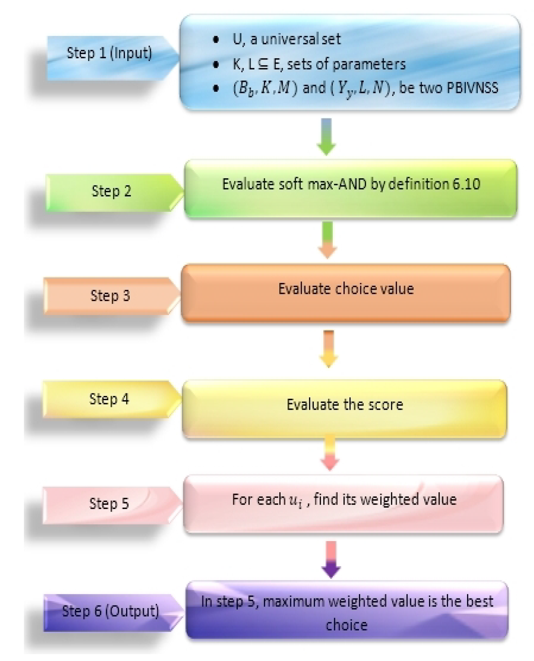
7. Algorithms
| Algorithm 1 Soft max-AND operations |
Step 1: We have two and (where and on universal set . Step 2: Evaluate
Step 3: Evaluate the choice value defined as: Step 4: Evaluate the score defined as: Step 5: For each it’s weighted value is: Step 6: Now the optimal decision is: |
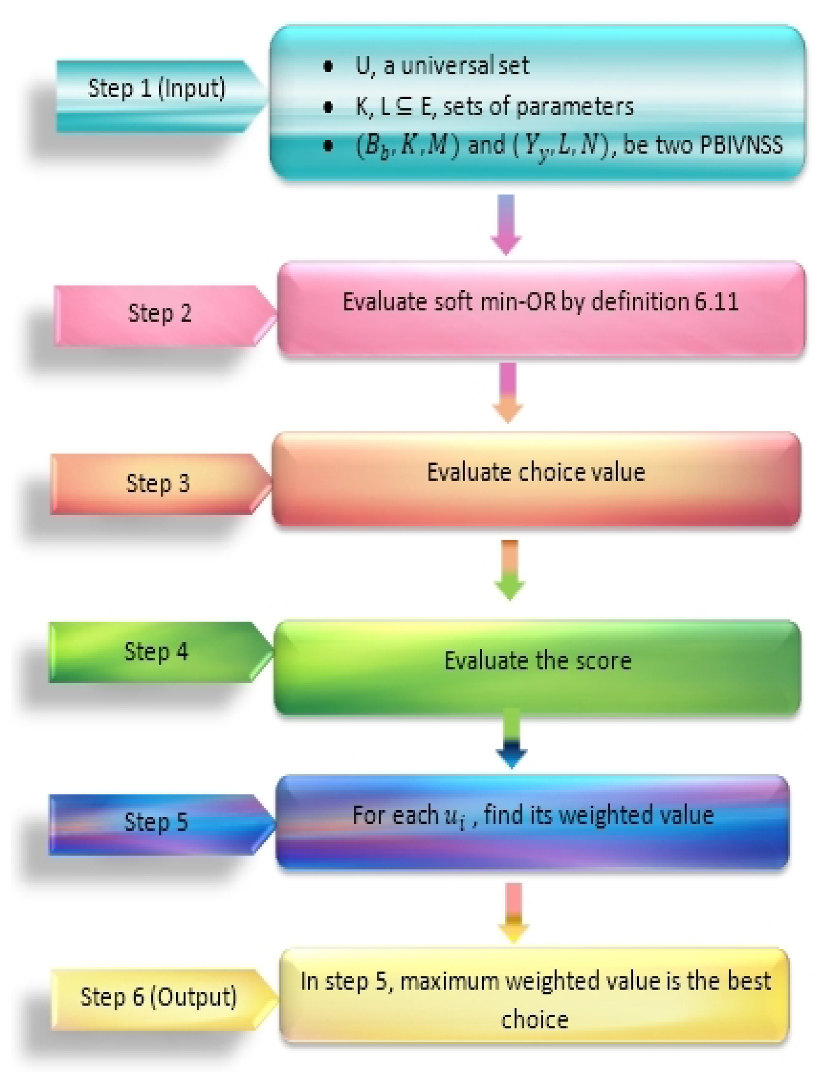
| Algorithm 2 Soft min-OR operations |
Step 1: Let we have two and (where and on universal set . Step 2: Evaluate
Step 3: Evaluate the choice value defined as: Step 4: Evaluate the score defined as: Step 5: For each it’s weighted value is: Step 6: Now the optimal decision is: |
8. Applications
| (Grading, Interval Value) | (Grading, Interval Value) | ||
| (3, [0.46,1.20]) | (3, [0.66,1.23]) | ||
| (3, [0.73,1.56]) | (3, [0.76,1.53]) | ||
| (4, [0.50,0.90]) | (4, [0.63,0.83]) | ||
| (2, [0.73,1.36]) | (2, [0.56,1.06]) | ||
| (6, [1.16,1.63]) | (6, [0.86,1.50]) | ||
| (3, [0.60,1.50]) | (1, [0.53,1.66]) | ||
| (1, [0.43,1.40]) | (0, [0.46,1.46]) | ||
| (3, [1.13,1.70]) | (3, [1.13,1.66]) | ||
| (6, [0.43,1.13]) | (6, [0.56,1.06]) | ||
| (5, [1.06,1.40]) | (5, [0.76,1.10]) | ||
| (1, [1.00,1.40]) | (1, [0.76,1.26]) | ||
| (3, [1.06,1.40]) | (3, [0.96,1.53]) | ||
| (1, [0.46,1.16]) | (1, [0.53,1.20]) | ||
| (5, [1.03,1.36]) | (5, [0.90,1.33]) | ||
| (1, [0.60,1.26]) | (2, [0.80,1.13]) | ||
| (6, [0.60,0.93]) | (6, [0.43,0.76]) | ||
| (4, [1.10,1.46]) | (4, [0.83,1.36]) | ||
| (6, [0.73,1.46]) | (6, [0.63,1.63]) |
| The Score | The Score | ||
| −52.14 | −10.34 | ||
| 31.02 | 42.46 | ||
| −102.18 | −79.3 | ||
| 4.41 | −41.8 | ||
| 158.76 | 84.6 | ||
| 5.94 | 25.27 | ||
| −48.64 | −21.24 | ||
| 79.12 | 92.92 | ||
| −150.48 | −107.28 | ||
| 37.82 | −47.74 | ||
| 16.34 | −11.02 | ||
| 28.06 | 51.52 | ||
| −55.89 | −27.6 | ||
| 70.08 | 59.2 | ||
| −22.77 | 1.25 | ||
| −106.92 | −158.04 | ||
| 93.09 | 46.69 | ||
| 35.64 | 73.08 |
| (Grading, Interval Value) | (Grading, Interval Value) | ||
| (1, [0.73,1.40]) | (0, [0.73,1.46]) | ||
| (1, [0.96,1.63]) | (1, [0.93,1.66]) | ||
| (1, [0.70,1.20]) | (2, [0.86,1.06]) | ||
| (1, [0.96,1.43]) | (1, [0.63,1.33]) | ||
| (0, [1.23,1.76]) | (1, [1.03,1.60]) | ||
| (0, [0.80,1.60]) | (0, [0.86,1.73]) | ||
| (0, [0.46,1.50]) | (0, [0.63,1.53]) | ||
| (2, [1.26,1.70]) | (2, [1.26,1.73]) | ||
| (1, [0.56,1.36]) | (2, [0.73,1.23]) | ||
| (2, [1.13,1.50]) | (2, [0.93,1.40]) | ||
| (0, [1.20,1.60]) | (1, [0.93,1.43]) | ||
| (3, [1.13,1.50]) | (1, [1.23,1.66]) | ||
| (1, [0.53,1.33]) | (0, [0.66,1.40]) | ||
| (3, [1.06,1.53]) | (3, [1.20,1.56]) | ||
| (0, [0.80,1.43]) | (0, [0.90,1.36]) | ||
| (2, [0.90,1.16]) | (2, [0.56,0.93]) | ||
| (0, [1.20,1.63]) | (1, [0.96,1.43]) | ||
| (3, [0.86,1.53]) | (1, [0.96,1.66]) |
| The Score | The Score | ||
| −9.72 | −3.7 | ||
| 6.84 | 11.62 | ||
| −18 | −28.32 | ||
| −0.36 | −14.84 | ||
| 14.16 | 13.3 | ||
| 0 | 8.3 | ||
| −25.12 | −13.84 | ||
| 37.18 | 39 | ||
| −33.8 | −35.16 | ||
| 11.44 | −8.52 | ||
| 15.2 | −4.77 | ||
| 15.84 | 23.85 | ||
| −30.8 | −8.54 | ||
| 28.44 | 53.64 | ||
| −5.22 | −0.14 | ||
| −22.4 | −60.32 | ||
| 27.18 | 6.84 | ||
| 6.84 | 19.26 |
| (Grading, Interval Value) | (Grading, Interval Value) | ||
| (5, [0.53,1.33]) | (5, [0.83,1.23]) | ||
| (6, [0.66,1.46]) | (4, [1.10,1.63]) | ||
| (3, [0.40,0.80]) | (4, [0.46,0.96]) | ||
| (7, [0.40,0.86]) | (7, [0.86,1.43]) | ||
| (4, [0.76,1.56]) | (4, [0.90,1.50]) | ||
| (3, [0.63,1.30]) | (5, [0.53,1.73]) | ||
| (2, [0.76,1.16]) | (3, [0.43,1.13]) | ||
| (3, [0.53,1.53]) | (2, [0.73,1.06]) | ||
| (0, [0.30,1.73]) | (6, [0.63,1.03]) | ||
| (5, [0.76,1.10]) | (5, [0.40,1.30]) | ||
| (4, [0.90,1.60]) | (6, [0.67,1.50]) | ||
| (3, [0.63,1.16]) | (3, [0.93,1.23]) | ||
| (7, [0.93,1.33]) | (7, [0.60,1.13]) | ||
| (4, [0.66,1.53]) | (4, [0.56,1.23]) | ||
| (5, [0.20,1.03]) | (2, [0.73,1.53]) | ||
| (3, [0.40,1.00]) | (4, [0.63,1.13]) | ||
| (4, [0.60,1.06]) | (3, [0.53,1.53]) | ||
| (6, [0.83,1.30]) | (2, [0.73,1.10]) | ||
| (5, [0.50,1.43]) | (5, [1.10,1.43]) | ||
| (6, [0.93,1.46]) | (4, [0.70,1.30]) | ||
| (3, [1.90,1.26]) | (3, [0.73,1.33]) | ||
| (7, [0.43,1.00]) | (7, [0.73,1.26]) | ||
| (4, [0.93,1.50]) | (4, [0.66,1.56]) | ||
| (4, [0.46,1.06]) | (5, [0.53,1.70]) | ||
| (2, [0.73,1.26]) | (3, [0.60,1.23]) | ||
| (4, [0.70,1.46]) | (2, [0.46,0.86]) | ||
| (1, [0.73,1.13]) | (6, [1.00,1.46]) |
| The Score | The Score | ||
| 15.51 | 4.2 | ||
| 75.11 | 104 | ||
| −97.72 | −92.5 | ||
| −131.46 | 74.76 | ||
| 96.9 | 73.2 | ||
| 24.92 | 52.8 | ||
| −12.16 | −72.8 | ||
| 4.2 | −32.94 | ||
| 0.34 | −74 | ||
| −30 | −53.13 | ||
| 71 | 44.77 | ||
| −29.82 | 32.2 | ||
| 112.98 | −60.06 | ||
| 68.1 | −32.1 | ||
| −115.17 | 47.25 | ||
| −71.63 | −42 | ||
| −27.3 | 2.64 | ||
| 70.67 | −26.46 | ||
| −9.24 | 88.2 | ||
| 91.76 | −6 | ||
| 31.9 | 2.64 | ||
| −137.76 | −4.62 | ||
| 81.6 | 38.1 | ||
| −82.2 | 43.89 | ||
| −5.88 | −29.96 | ||
| 18.5 | −111.51 | ||
| −21.2 | 100.27 |
| (Grading, Interval Value) | (Grading, Interval Value) | ||
| (1, [0.66,1.46]) | (3, [0.96,1.36]) | ||
| (3, [0.83,1.53]) | (2, [1.30,1.66]) | ||
| (0, [0.60,0.90]) | (3, [0.53,1.03]) | ||
| (2, [0.50,1.03]) | (0, [1.03,1.46]) | ||
| (4, [0.83,1.63]) | (4, [1.00,1.60]) | ||
| (2, [0.76,1.40]) | (1, [0.86,1.76]) | ||
| (1, [0.93,1.33]) | (3, [0.56,1.16]) | ||
| (1, [0.56,1.56]) | (2, [0.96,1.33]) | ||
| (0, [0.40,0.76]) | (4, [0.76,1.16]) | ||
| (2, [0.93,1.30]) | (4, [0.50,1.40]) | ||
| (4, [1.10,1.70]) | (3, [0.83,1.60]) | ||
| (3, [0.76,1.23]) | (2, [1.06,1.46]) | ||
| (1, [1.06,1.36]) | (3, [0.90,1.26]) | ||
| (3, [0.83,1.56]) | (0, [0.73,1.46]) | ||
| (0, [0.20,1.36]) | (1, [0.96,1.66]) | ||
| (2, [0.50,1.10]) | (2, [0.76,1.26]) | ||
| (2, [0.70,1.33]) | (1, [0.56,1.66]) | ||
| (3, [0.96,1.30]) | (0, [0.96,1.40]) | ||
| (0, [0.60,1.56]) | (3, [1.20,1.46]) | ||
| (4, [0.96,1.53]) | (0, [1.00,1.50]) | ||
| (1, [1.10,1.53]) | (1, [0.96,1.56]) | ||
| (3, [0.56,1.10]) | (4, [0.96,1.33]) | ||
| (2, [1.06,1.70]) | (3, [0.83,1.63]) | ||
| (2, [0.53,1.23]) | (2, [0.86,1.70]) | ||
| (0, [0.86,1.43]) | (3, [0.90,1.36]) | ||
| (1, [0.80,1.63]) | (0, [0.53,1.03]) | ||
| (0, [0.96,1.46]) | (1, [1.10,1.63]) |
| The Score | The Score | ||
| 7.67 | −1.08 | ||
| 38.57 | 52.92 | ||
| −37.56 | −83.16 | ||
| −44.25 | 18.2 | ||
| 63.12 | 47.04 | ||
| 12.45 | 31.2 | ||
| 12 | −66.4 | ||
| 1.92 | 1.7 | ||
| −61.6 | −50.88 | ||
| 12.3 | −58.08 | ||
| 101.76 | 14.44 | ||
| −11.78 | 20.8 | ||
| 27.12 | −16.34 | ||
| 37.44 | −8.84 | ||
| −31.9 | 26.6 | ||
| −37.24 | −28.08 | ||
| −1.12 | −8.64 | ||
| 23.4 | −0.84 | ||
| −6 | 30.24 | ||
| 35.52 | 5.04 | ||
| 30.16 | 7.56 | ||
| −66.5 | −2.88 | ||
| 46.5 | 17.1 | ||
| −43.5 | 24 | ||
| −2.16 | −5.7 | ||
| 6.6 | −58.5 | ||
| 4.86 | 35.28 |
9. Conclusions
Author Contributions
Funding
Data Availability Statement
Conflicts of Interest
References
- Xiao, F.; Zhang, Z.; Abawajy, J. Workflow scheduling in distributed systems under fuzzy environment. J. Intell. Fuzzy Syst. 2019, 37, 5323–5333. [Google Scholar] [CrossRef]
- Cao, Z.; Lin, C.T.; Lai, K.L.; Ko, L.W.; King, J.T.; Liao, K.K.; Fuh, J.L.; Wang, S.J. Extraction of SSVEPs-based inherent fuzzy entropy using a wearable headband EEG in migraine patients. IEEE Trans. Fuzzy Syst. 2019, 28, 14–27. [Google Scholar] [CrossRef] [Green Version]
- Liu, F.; Gao, X.; Zhao, J.; Deng, Y. Generalized belief entropy and its application in identifying conflict evidence. IEEE Access 2019, 7, 126625–126633. [Google Scholar] [CrossRef]
- Seiti, H.; Hafezalkotob, A.; Najafi, S.E.; Khalaj, M. A risk-based fuzzy evidential framework for FMEA analysis under uncertainty: An interval-valued DS approach. J. Intell. Fuzzy Syst. 2018, 35, 1419–1430. [Google Scholar] [CrossRef]
- Wang, Q.; Li, Y.; Liu, X. Analysis of feature fatigue EEG signals based on wavelet entropy. Int. J. Pattern Recognit. Artif. Intell. 2018, 32, 1854023. [Google Scholar] [CrossRef]
- Jiang, W.; Cao, Y.; Deng, X. A novel Z-network model based on Bayesian network and Z-number. IEEE Trans. Fuzzy Syst. 2019, 28, 1585–1599. [Google Scholar] [CrossRef]
- Fu, C.; Chang, W.; Xue, M.; Yang, S. Multiple criteria group decision making with belief distributions and distributed preference relations. Eur. J. Oper. Res. 2019, 273, 623–633. [Google Scholar] [CrossRef]
- Gao, X.; Deng, Y. Quantum model of mass function. Int. J. Intell. Syst. 2020, 35, 267–282. [Google Scholar] [CrossRef]
- Luo, Z.; Deng, Y. A vector and geometry interpretation of basic probability assignment in Dempster-Shafer theory. Int. J. Intell. Syst. 2020, 35, 944–962. [Google Scholar] [CrossRef]
- Zadeh, L.A. Information and control. Fuzzy Sets 1965, 8, 338–353. [Google Scholar]
- Fei, L. On interval-valued fuzzy decision-making using soft likelihood functions. Int. J. Intell. Syst. 2019, 34, 1631–1652. [Google Scholar] [CrossRef]
- Song, Y.; Wang, X.; Quan, W.; Huang, W. A new approach to construct similarity measure for intuitionistic fuzzy sets. Soft Comput. 2019, 23, 1985–1998. [Google Scholar] [CrossRef]
- Xue, Y.; Deng, Y. Entailment for intuitionistic fuzzy sets based on generalized belief structures. Int. J. Intell. Syst. 2020, 35, 963–982. [Google Scholar] [CrossRef]
- Zhou, D.; Al-Durra, A.; Zhang, K.; Ravey, A.; Gao, F. A robust prognostic indicator for renewable energy technologies: A novel error correction grey prediction model. IEEE Trans. Ind. Electron. 2019, 66, 9312–9325. [Google Scholar] [CrossRef]
- Molodtsov, D. Soft set theory—First results. Comput. Math. Appl. 1999, 37, 19–31. [Google Scholar] [CrossRef] [Green Version]
- Feng, F.; Cho, J.; Pedrycz, W.; Fujita, H.; Herawan, T. Soft set based association rule mining. Knowl.-Based Syst. 2016, 111, 268–282. [Google Scholar] [CrossRef]
- Feng, F.; Li, Y. Soft subsets and soft product operations. Inf. Sci. 2013, 232, 44–57. [Google Scholar] [CrossRef]
- Xu, W.; Ma, J.; Wang, S.; Hao, G. Vague soft sets and their properties. Comput. Math. Appl. 2010, 59, 787–794. [Google Scholar] [CrossRef] [Green Version]
- Maji, P.K.; Biswas, R.; Roy, A.R. Soft set theory. Comput. Math. Appl. 2003, 45, 555–562. [Google Scholar] [CrossRef] [Green Version]
- Majumdar, P.; Samanta, S.K. Generalised fuzzy soft sets. Comput. Math. Appl. 2010, 59, 1425–1432. [Google Scholar] [CrossRef] [Green Version]
- Maji, P.K.; Biswas, R.; Roy, A.R. Intuitionistic fuzzy soft sets. J. Fuzzy Math. 2001, 9, 677–692. [Google Scholar]
- Maji, P.K. More on intuitionistic fuzzy soft sets. In International Workshop on Rough Sets, Fuzzy Sets, Data Mining, and Granular-Soft Computing; Springer: Berlin/Heidelberg, Germany, 2009; pp. 231–240. [Google Scholar]
- Dinda, B.; Bera, T.; Samanta, T.K. Generalised intuitionistic fuzzy soft sets and its application in decision making. arXiv 2010, arXiv:1010.2468. [Google Scholar]
- Dempster, A.P. Upper and lower probabilities induced by a multivalued mapping. In Classic Works of the Dempster-Shafer Theory of Belief Functions; Springer: Berlin/Heidelberg, Germany, 2008; pp. 57–72. [Google Scholar]
- Cheng, C.; Cao, Z.; Xiao, F. A generalized belief interval-valued soft set with applications in decision making. Soft Comput. 2020, 24, 9339–9350. [Google Scholar] [CrossRef]
- Jiang, Y.; Tang, Y.; Chen, Q.; Liu, H.; Tang, J. Interval-valued intuitionistic fuzzy soft sets and their properties. Comput. Math. Appl. 2010, 60, 906–918. [Google Scholar] [CrossRef] [Green Version]
- Khalil, A.M.; Li, S.G.; Garg, H.; Li, H.; Ma, S. New operations on interval-valued picture fuzzy set, interval-valued picture fuzzy soft set and their applications. IEEE Access 2019, 7, 51236–51253. [Google Scholar] [CrossRef]
- Deli, I. Interval-valued neutrosophic soft sets and its decision making. Int. J. Mach. Learn. Cybern. 2017, 8, 665–676. [Google Scholar] [CrossRef] [Green Version]
- Khan, M.J.; Kumam, P.; Ashraf, S.; Kumam, W. Generalized picture fuzzy soft sets and their application in decision support systems. Symmetry 2019, 11, 415. [Google Scholar] [CrossRef] [Green Version]
- Alkhazaleh, S.; Salleh, A.R.; Hassan, N. Possibility fuzzy soft set. Adv. Decis. Sci. 2011, 2011, 479756. [Google Scholar] [CrossRef]
- Khalil, A.M.; Li, S.G.; Li, H.X.; Ma, S.Q. Possibility m-polar fuzzy soft sets and its application in decision-making problems. J. Intell. Fuzzy Syst. 2019, 37, 929–940. [Google Scholar] [CrossRef]
- Jia-hua, D.; Zhang, H.; He, Y. Possibility Pythagorean fuzzy soft set and its application. J. Intell. Fuzzy Syst. 2019, 36, 413–421. [Google Scholar] [CrossRef]
- Karaaslan, F. Possibility neutrosophic soft sets and PNS-decision making method. Appl. Soft Comput. 2017, 54, 403–414. [Google Scholar] [CrossRef] [Green Version]
- Zhang, H.D.; Shu, L. Possibility multi-fuzzy soft set and its application in decision making. J. Intell. Fuzzy Syst. 2014, 27, 2115–2125. [Google Scholar] [CrossRef]
- Shafer, G. A Mathematical Theory of Evidence; Princeton University Press: Princeton, NJ, USA, 1976; Volume 42. [Google Scholar]
- Shenoy, P.P. Using Dempster-Shafer’s belief-function theory in expert systems. In Applications of Artificial Intelligence X: Knowledge-Based Systems; International Society for Optics and Photonics: Bellingham, WA, USA, March 1992; Volume 1707, pp. 2–14. [Google Scholar]
- Huang, Z.; Yang, L.; Jiang, W. Uncertainty measurement with belief entropy on the interference effect in the quantum-like Bayesian Networks. Appl. Math. Comput. 2019, 347, 417–428. [Google Scholar] [CrossRef] [Green Version]
- Zhou, M.; Liu, X.B.; Chen, Y.W.; Yang, J.B. Evidential reasoning rule for MADM with both weights and reliabilities in group decision making. Knowl.-Based Syst. 2018, 143, 142–161. [Google Scholar] [CrossRef]
- Zhou, M.; Liu, X.B.; Yang, J.B.; Chen, Y.W.; Wu, J. Evidential reasoning approach with multiple kinds of attributes and entropy-based weight assignment. Knowl.-Based Syst. 2019, 163, 358–375. [Google Scholar] [CrossRef]
- Kang, B.; Zhang, P.; Gao, Z.; Chhipi-Shrestha, G.; Hewage, K.; Sadiq, R. Environmental assessment under uncertainty using Dempster–Shafer theory and Z-numbers. J. Ambient. Intell. Humaniz. Comput. 2020, 11, 2041–2060. [Google Scholar] [CrossRef]
- He, Z.; Jiang, W. An evidential dynamical model to predict the interference effect of categorization on decision making results. Knowl.-Based Syst. 2018, 150, 139–149. [Google Scholar] [CrossRef]
- Zhou, M.; Liu, X.; Yang, J. Evidential reasoning approach for MADM based on incomplete interval value. J. Intell. Fuzzy Syst. 2017, 33, 3707–3721. [Google Scholar] [CrossRef] [Green Version]
- Liu, Z.G.; Pan, Q.; Dezert, J.; Martin, A. Combination of classifiers with optimal weight based on evidential reasoning. IEEE Trans. Fuzzy Syst. 2017, 26, 1217–1230. [Google Scholar] [CrossRef] [Green Version]
- Pan, L.; Deng, Y. An association coefficient of a belief function and its application in a target recognition system. Int. J. Intell. Syst. 2020, 35, 85–104. [Google Scholar] [CrossRef]
- Fatimah, F.; Rosadi, D.; Hakim, R.F.; Alcantud, J.C.R. N-soft sets and their decision making algorithms. Soft Comput. 2018, 22, 3829–3842. [Google Scholar] [CrossRef]
- Akram, M.; Adeel, A.; Alcantud, J.C.R. Group decision-making methods based on hesitant N-soft sets. Expert Syst. Appl. 2019, 115, 95–105. [Google Scholar] [CrossRef]
- Akram, M.; Adeel, A.; Alcantud, J.C.R. Fuzzy N-soft sets: A novel model with applications. J. Intell. Fuzzy Syst. 2018, 35, 4757–4771. [Google Scholar] [CrossRef]
- Zeng, S.; Shoaib, M.; Ali, S.; Smarache, F.; Rashmanlou, H.; Mofidnakhaei, F. Certain properties of singlevalued neutrosophic graph with application in food and agriculture organization. Int. J. Comput. Intell. Syst. 2021, 14, 1516–1540. [Google Scholar] [CrossRef]
- Gulfam, M.; Mahmood, M.K.; Smarandache, F.; Ali, S. New Dombi aggregation operators on bipolar neutrosophic set with application in multi-attribute decision-making problems. J. Intell. Fuzzy Syst. 2021, 40, 5043–5060. [Google Scholar] [CrossRef]
- Hameed, M.S.; Mukhtar, S.; Khan, H.N.; Ali, S.; Mateen, M.H.; Gulzar, M. Pythagorean fuzzy N-Soft groups. Int. J. Electr. Comput. Eng. 2021, 21, 1030–1038. [Google Scholar]
- Liu, J.B.; Ali, S.; Mahmood, M.K.; Mateen, M.H. On m-polar diophantine fuzzy Nsoft set with applications. Comb. Chem. High Throughput Screen. 2020, 23. [Google Scholar] [CrossRef] [PubMed]
- Zeng, S.; Shoaib, M.; Ali, S.; Abbas, Q.; Nadeem, M.S. Complex vague graphs and their application in decision-making problems. IEEE Access 2020, 8, 174094–174104. [Google Scholar] [CrossRef]
- Mahmood, M.K.; Zeng, S.; Gulfam, M.; Ali, S.; Jin, Y. Bipolar neutrosophic dombi aggregation operators with application in multi-attribute decision making problems. IEEE Access 2020, 8, 156600–156614. [Google Scholar] [CrossRef]
- Akram, M.; Amjad, U.; Davvaz, B. Decision-making analysis based on bipolar fuzzy N-soft information. Comput. Appl. Math. 2021, 40, 182. [Google Scholar] [CrossRef]
- Akram, M.; Luqman, A.; Kahraman, C. Hesitant Pythagorean fuzzy ELECTRE-II method for multi-criteria decision-making problems. Appl. Soft Comput. 2021, 108, 107479. [Google Scholar] [CrossRef]
- Adeel, A.; Akram, M.; Cagman, N. Decision-making analysis based on hesitant fuzzy N-Soft ELECTRE-I approach. Soft Comput. 2021. [Google Scholar] [CrossRef]
- Akram, M.; Kahraman, C.; Zahid, K. Extension of TOPSIS model to the decision-making under complex spherical fuzzy information. Soft Comput. 2021, 25, 10771–10795. [Google Scholar] [CrossRef]
- Akram, M.; Alsulami, S.; Zahid, K. A hybrid method for complex pythagorean fuzzy decision making. Math. Probl. Eng. 2021, 2021, 9915432. [Google Scholar] [CrossRef]
- Liu, Y.T.; Pal, N.R.; Marathe, A.R.; Lin, C.T. Weighted fuzzy Dempster–Shafer framework for multimodal information integration. IEEE Trans. Fuzzy Syst. 2017, 26, 338–352. [Google Scholar] [CrossRef]
- Gong, Y.; Su, X.; Qian, H.; Yang, N. Research on fault diagnosis methods for the reactor coolant system of nuclear power plant based on DS evidence theory. Ann. Nucl. Energy 2018, 112, 395–399. [Google Scholar] [CrossRef]
- Mo, H.; Deng, Y. Identifying node importance based on evidence theory in complex networks. Phys. A Stat. Mech. Its Appl. 2019, 529, 121538. [Google Scholar] [CrossRef]
- Seiti, H.; Hafezalkotob, A. Developing pessimistic–optimistic risk-based methods for multi-sensor fusion: An interval-valued evidence theory approach. Appl. Soft Comput. 2018, 72, 609–623. [Google Scholar] [CrossRef]
- Deng, X.; Jiang, W.; Wang, Z. Zero-sum polymatrix games with link uncertainty: A Dempster-Shafer theory solution. Appl. Math. Comput. 2019, 340, 101–112. [Google Scholar] [CrossRef]
- Xiao, F. A new divergence measure for belief functions in D–S evidence theory for multisensor data fusion. Inf. Sci. 2020, 514, 462–483. [Google Scholar] [CrossRef]
- Xiao, F. EFMCDM: Evidential fuzzy multicriteria decision making based on belief entropy. IEEE Trans. Fuzzy Syst. 2019, 28, 1477–1491. [Google Scholar] [CrossRef]
- Cui, H.; Liu, Q.; Zhang, J.; Kang, B. An improved deng entropy and its application in pattern recognition. IEEE Access 2019, 7, 18284–18292. [Google Scholar] [CrossRef]
- Ozkan, K. Comparing Shannon entropy with Deng entropy and improved Deng entropy for measuring biodiversity when a priori data is not clear. Forestist 2018, 68, 136–140. [Google Scholar]
- Xiao, F. Generalization of Dempster-Shafer theory: A complex belief function. arXiv 2019, arXiv:1906.11409. [Google Scholar]
- Jiang, W. A correlation coefficient for belief functions. Int. J. Approx. Reason. 2018, 103, 94–106. [Google Scholar] [CrossRef] [Green Version]


Publisher’s Note: MDPI stays neutral with regard to jurisdictional claims in published maps and institutional affiliations. |
© 2021 by the authors. Licensee MDPI, Basel, Switzerland. This article is an open access article distributed under the terms and conditions of the Creative Commons Attribution (CC BY) license (https://creativecommons.org/licenses/by/4.0/).
Share and Cite
Ali, S.; Kousar, M.; Xin, Q.; Pamučar, D.; Hameed, M.S.; Fayyaz, R. Belief and Possibility Belief Interval-Valued N-Soft Set and Their Applications in Multi-Attribute Decision-Making Problems. Entropy 2021, 23, 1498. https://doi.org/10.3390/e23111498
Ali S, Kousar M, Xin Q, Pamučar D, Hameed MS, Fayyaz R. Belief and Possibility Belief Interval-Valued N-Soft Set and Their Applications in Multi-Attribute Decision-Making Problems. Entropy. 2021; 23(11):1498. https://doi.org/10.3390/e23111498
Chicago/Turabian StyleAli, Shahbaz, Muneeba Kousar, Qin Xin, Dragan Pamučar, Muhammad Shazib Hameed, and Rabia Fayyaz. 2021. "Belief and Possibility Belief Interval-Valued N-Soft Set and Their Applications in Multi-Attribute Decision-Making Problems" Entropy 23, no. 11: 1498. https://doi.org/10.3390/e23111498
APA StyleAli, S., Kousar, M., Xin, Q., Pamučar, D., Hameed, M. S., & Fayyaz, R. (2021). Belief and Possibility Belief Interval-Valued N-Soft Set and Their Applications in Multi-Attribute Decision-Making Problems. Entropy, 23(11), 1498. https://doi.org/10.3390/e23111498