1. Introduction
Multi-input multi-output (MIMO) systems, defined as systems with multiple control inputs and outputs, are widely used in industrial systems. Many common industrial control systems can be modeled as MIMO systems, such as chemical reactors, distillers, generators, and automobile transmission systems [
1,
2,
3,
4,
5]. A consensus is that the control of the MIMO systems is more complex than the control of the single-input single-output (SISO) systems. In the MIMO systems, the outputs are affected by each input. In other words, there is a coupled interaction between the input and output variables of the MIMO systems. Due to the interaction in the MIMO systems, it is not easy to directly apply the advanced control methods based on the SISO systems.
Currently, the control strategies of the MIMO systems are mainly based on the methods of decoupling. Decoupling strategies can be divided into static decoupling and dynamic decoupling. The former achieves decoupling based on steady-state gain, which can effectively reduce the impact of model uncertainty, but the high-frequency response of MIMO systems is often not ideal [
6]. The dynamic decoupling can achieve a trade-off between complexity and decoupling performance. In recent years, various dynamic decoupling strategies have been developed, such as ideal decoupling, simplified decoupling, and reverse decoupling. The ideal decoupler can provide a simple decoupling system, but the ideal decoupler is difficult to realize in practical applications. The opposite is simplified decoupling. Although simplified decoupling can obtain simple decoupling and decoupling, the decoupling system will be very complicated. In [
7], Hagglund T proposed a decoupling method that approximates the sum of elements to reduce the system’s complexity after decoupling. Reverse decoupling takes into account the advantages of ideal decoupling and simplified decoupling. However, when there is a time-delay element in the MIMO systems, reverse decoupling cannot guarantee the system’s stability. In addition, researchers have used intelligent algorithms for MIMO systems and proposed various intelligent decoupling algorithms [
8,
9,
10,
11,
12]. However, because the design of this kind of method is difficult to understand and the controller is complicated, it is difficult for engineers to adopt.
As an algebraic design method, the CDM proposed by S. Manabe is simple and easy to implement [
13]. Compared with other control methods, CDM only requires the designer to define one parameter: the equivalent time constant [
14]. At the same time, all algebraic equations in the CDM are expressed in the form of polynomials, which facilitates the elimination of poles and zeros in the design and analysis of the control systems. CDM has been proven to be a method to ensure the robustness of the control system, and its effectiveness has been proven through a series of experiments [
15,
16,
17]. Therefore, with the continuous improvement of CDM, CDM has been continuously applied to existing control systems. Mohamed T. H. combined CDM with ecological optimization technology (ECO) for load frequency design in multi-regional power systems in [
18]. Experimental results show that the proposed method is robust in the presence of disturbance uncertainty. Because CDM is simple, effective and robust, it is also applied in MIMO system control [
19]. CDM was be used to design a PI controller with two cone-shaped official position research objects in [
20]. The simulation results prove the effectiveness of CDM on disturbance suppression. In [
21], CDM was used to solve the controller gain to suppress the vibration in the flexible robot system.
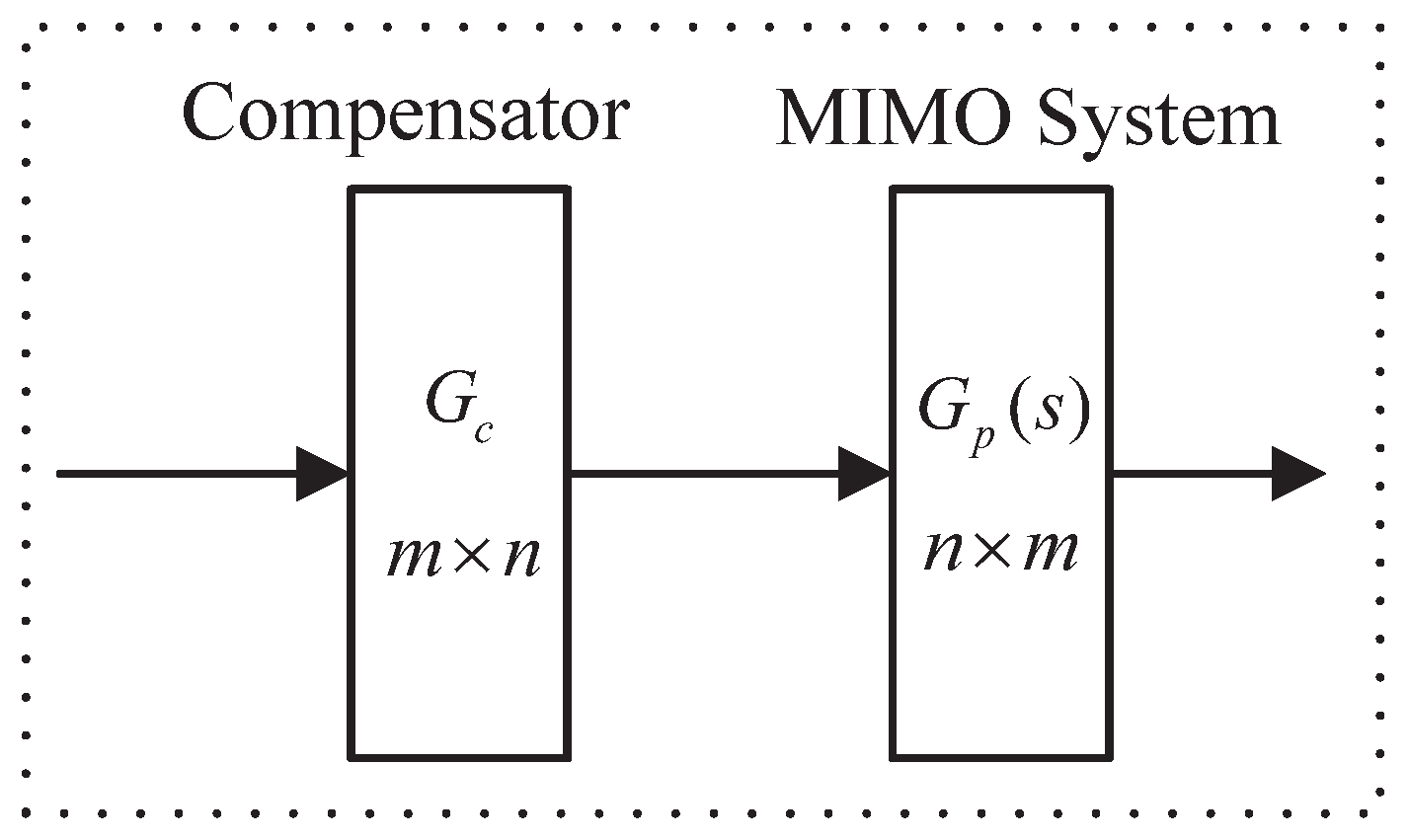
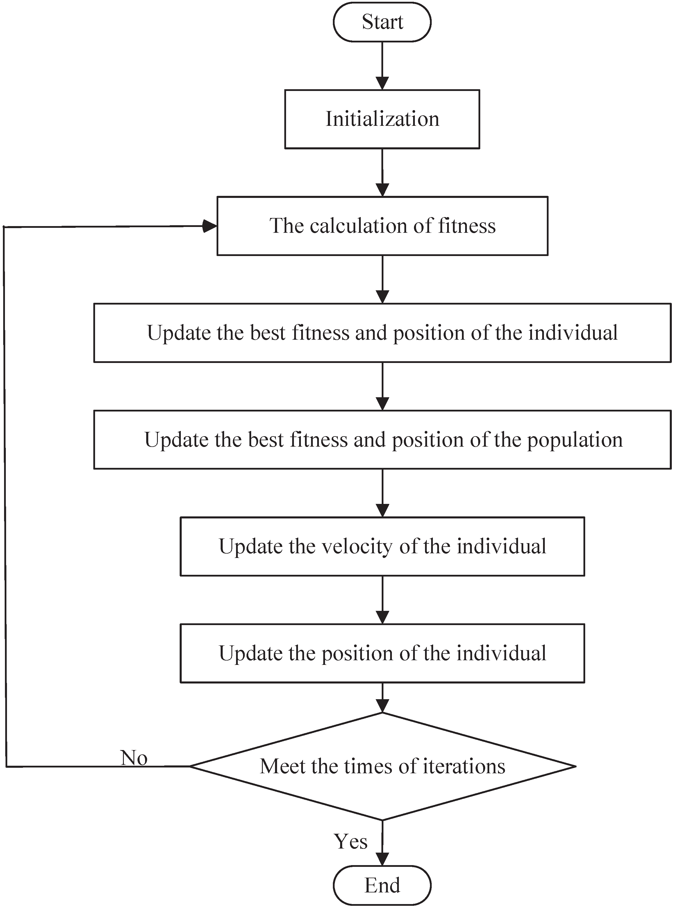
The first problem to be solved in the controller design of the MIMO system is how to achieve decoupling. Compared with other existing results, this article transforms the decoupling problem into the parameter optimization problem and gives an interaction measurement to evaluate the decoupling degree of the MIMO systems. The PSO algorithm is used to optimize the parameters of the compensator to achieve decoupling. After decoupling, the systems tend to have high order. The CDM considers the robustness and interference suppression performance of the system and the simplicity of design. Therefore, motivated by the advantages of CDM, this paper applies the CDM to the field of controller design for MIMO systems. At the same time, considering measurement noise can generate undesired control activity resulting in wear of actuators and reduced performance, this article analyzes the controller’s suppression effect on measurement noise based on the CDM. To verify the effectiveness and universality of the proposed method, this paper gives four typical design examples of MIMO systems in the hope of providing engineers and technicians a reference.
The main innovations of this paper are as follows:
- (1)
Converts the compensator design problem used for decoupling into parameter optimization problems to reduce the difficulty of decoupling.
- (2)
Gives an interaction measurement to quantify the interaction of coupled systems.
- (3)
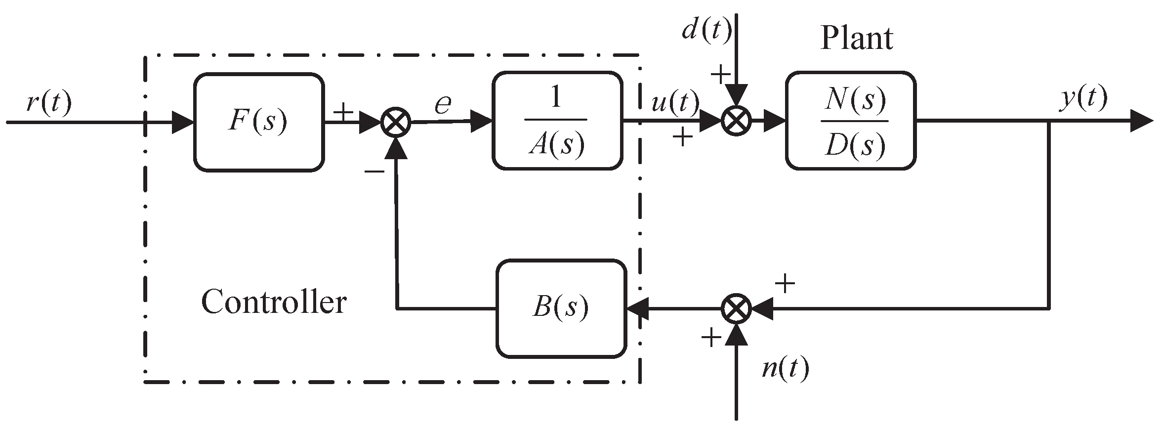
Analyzes the controller’s suppression effect on measurement noise based on the CDM.
- (4)
Research on the application of CDM methods to MIMO systems needs to be promoted. In order to make up for the shortcomings of existing research, this paper presents a design strategy of a robust controller based on CDM, which provides a reference for the design of the MIMO system controller in other articles.
The rest of this article is organized as follows:
Section 2 gives an interaction measurement of the coupling interaction and uses the PSO algorithm to design the compensator to achieve decoupling;
Section 3 summarizes the design process of the CDM controller and analyzes the controller’s suppression effect on measurement noise based on the CDM.
Section 4 outlines a set of controller design procedures for MIMO systems; four unique objects are simulated to verify the effectiveness of the proposed method in
Section 5. Finally, a conclusion is given.
5. Simulation Experiment
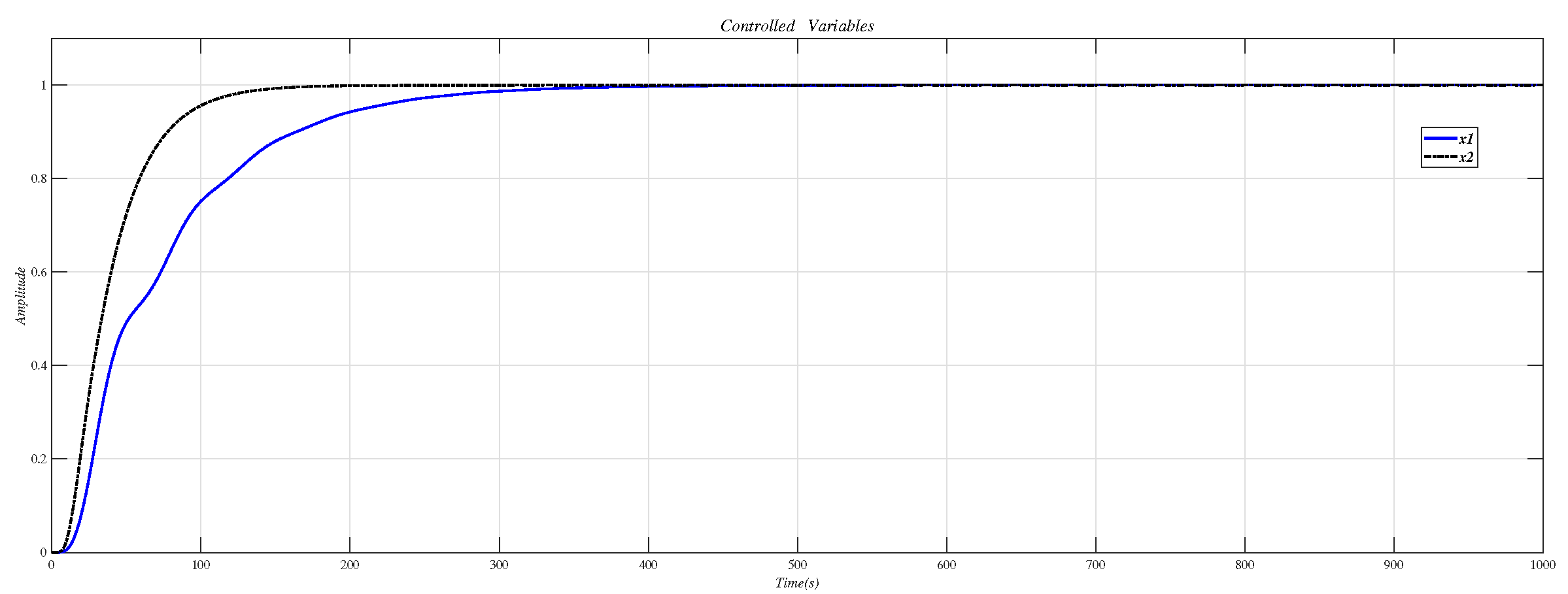
This section conducts simulation experiments on four unique control targets to prove the effectiveness of this method. The experiments are evaluated with a step response of 1. The state variable is set to , and the system output is set to . Use the compensator for decoupling. When the interaction of the MIMO system is minimized, treat it as n SISO systems, and set each SISO system as .
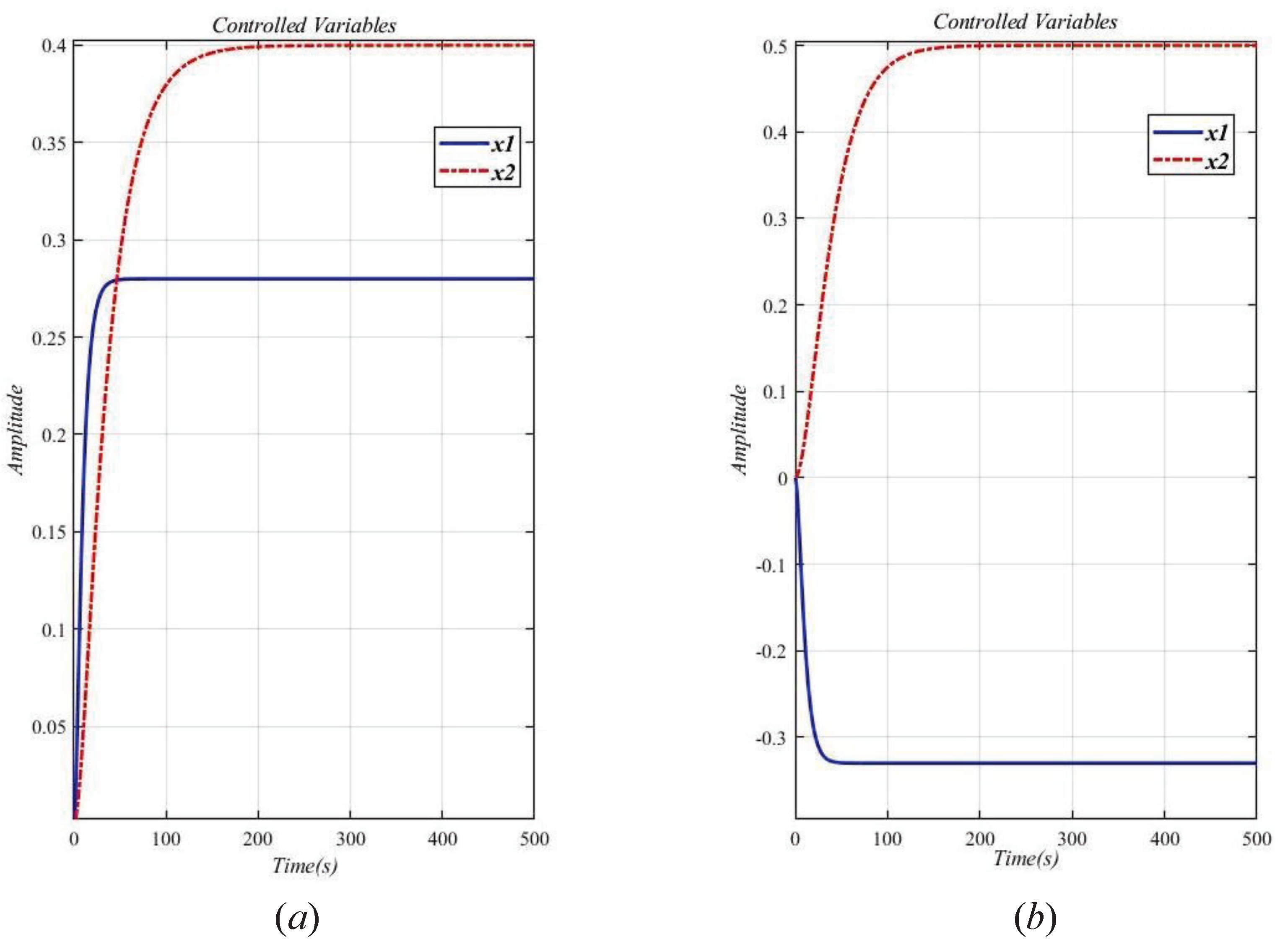
Example 2. Consider the two-input two-output second-order inertial system (sugar factory model) in [27]. The transfer function is: Without the decoupling design, the step response curve is shown in
Figure 8.
It can be seen from
Figure 8a that
. As shown in
Figure 8b,
. The two loops are obviously related, so the system (29) is a related system to the interaction. Therefore a decoupling design method is used to eliminate the interaction of the original system.
Select the angular frequency
, and obtain the compensator as Equation (
30).
Apply the compensator (30) to the original system (29), then the decoupling system
is obtained.
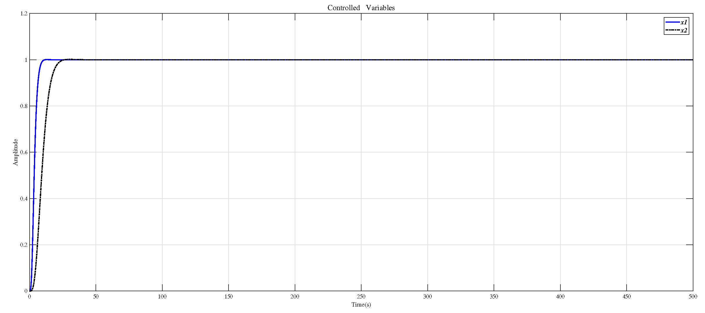
Figure 9 draws the step response curve of the original system (29) after the decoupling design. As can be seen from
Figure 9, the interaction of
is effectively suppressed, especially in the static response part of the system. However, there is still a weak interaction in the dynamic response part. Overall, the decoupling effect is good.
The two SISO systems after decoupling are set to
and
. For
and
, use the stability index
and equivalent time constant
in
Table 4 to calculate CDM control polynomial parameters.
Table 4 shows the equivalent time constant
and CDM control polynomial parameter values.
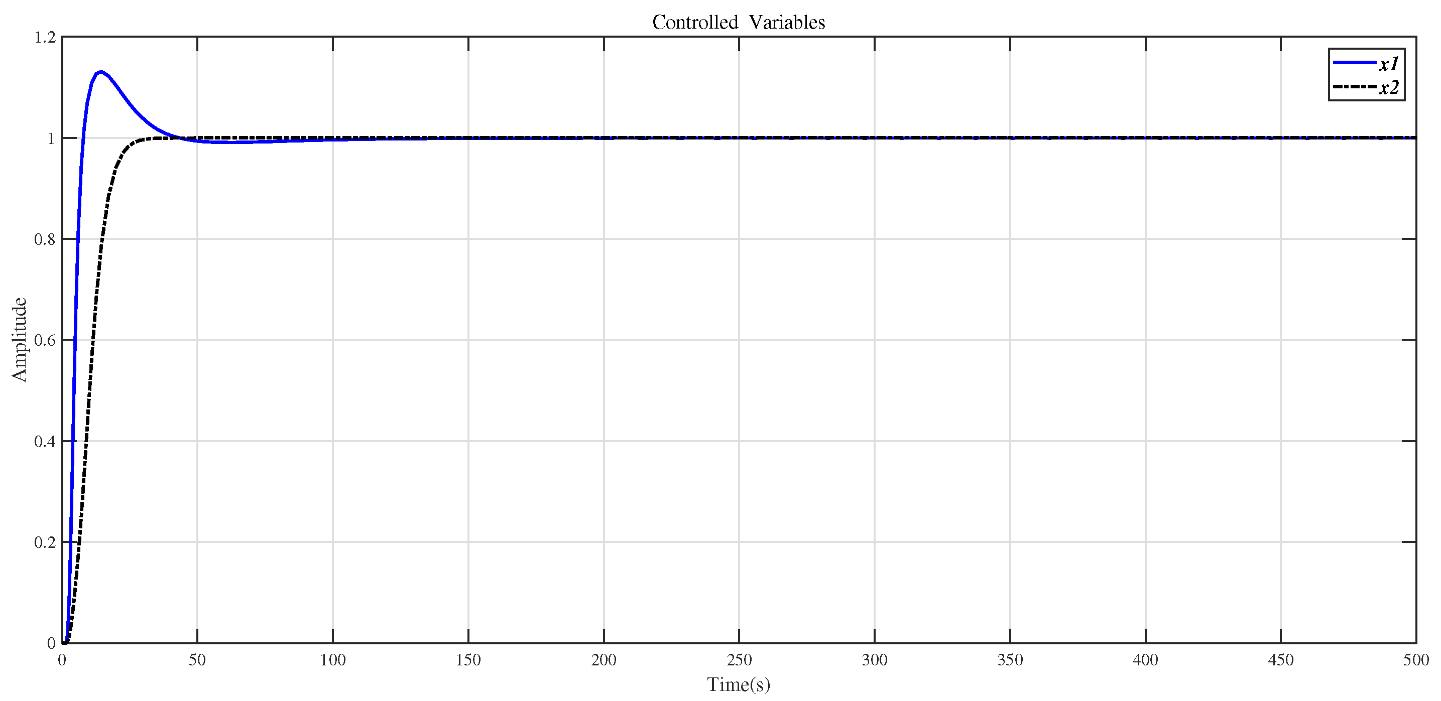
Using the CDM control polynomial parameters in
Table 4 to control
and
, the results are shown in
Figure 10.
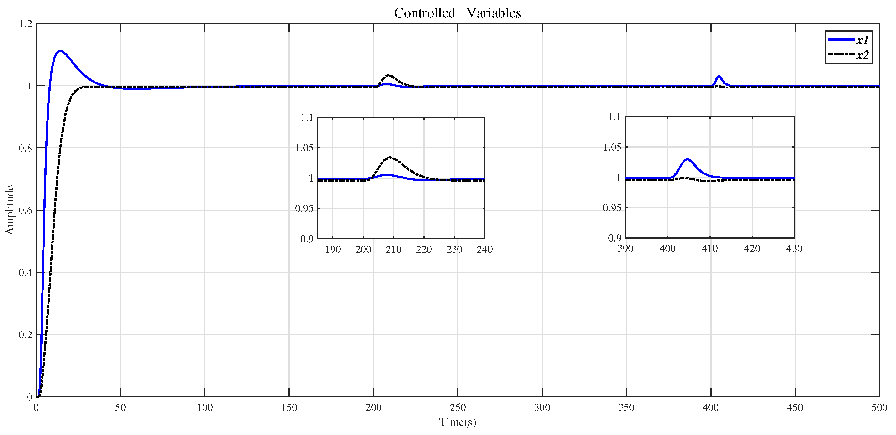
Figure 11 shows the result of inserting the compensator (30) in front of the controlled object (29) and using the CDM parameters in
Table 4 for control. Affected by the interaction of the dynamic response part, the system overshoot increases.
Here, the compensator (31) designed in [
27] is compared with the method in this paper.
Table 5 summarizes the results of evaluating the compensators (30) and (31) using formula (12).
Table 5 shows that the decoupling effect of the compensator designed by the method in this paper is better.
In [
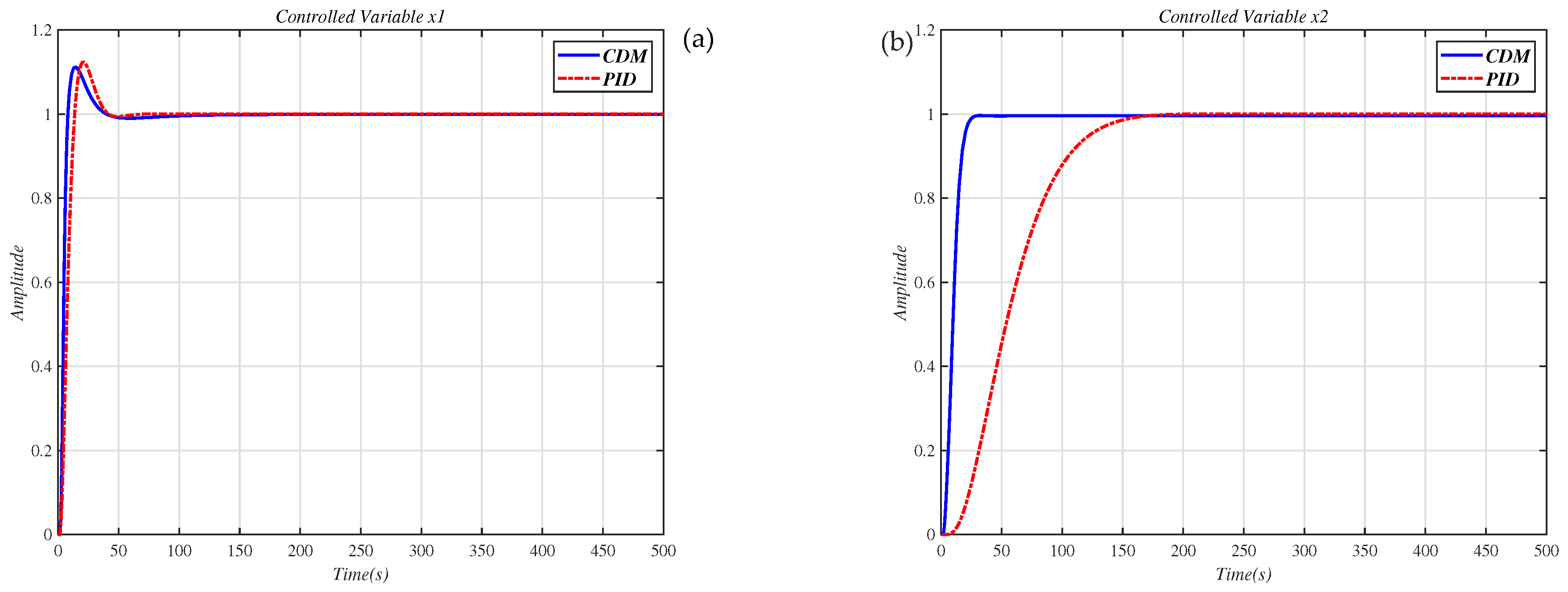
27], Masaya et al. designed a PID controller according to Shunji’s optimization method. We also use the design method proposed in [
27] to design the controller for the decoupling system
, which uses the compensator (30), and
Figure 12 shows the results of the Masaya-PID controller and the CDM controller in this paper to control the decoupling system
. From this figure and the performance values appearing in
Table 6, it is seen that the CDM controller has a more successful time-domain performance.
In order to verify the robustness of the method in this paper, the system with disturbances and modeling errors is simulated. When there is a step disturbance in the original system, the control result is shown in
Figure 13. According to
Figure 13, the influence of the disturbance signal subsides in a short time. Suppose that the correct system model is represented by Equation (
32), and the system model with errors is represented by Equation (
29). The changes in the parameter of Equation (
29) are in the interval
. The compensator (30) is applied to the correct system model (32), and the CDM controller is used to control. The experimental results are shown in
Figure 14. From the results in
Figure 14, it can be seen that when the model has measurement errors, the control effect of the method in this paper is good.
Figure 13 and
Figure 14 show that the method proposed in this paper is robust.
Example 3. The multivariable four-tank system has a tunable transmission of zero [28,29]. With appropriate "tuning", this system will exhibit nonminimum-phase characteristics. Applying the nominal operating parameters given in [28,29] yields the four-tank system model: For the four-tank system of the controlled object (33), the frequency
is selected, and the precompensator is obtained.
Use the evaluation formula (12) to evaluate the decoupling system after the compensator formula (34) acts on the controlled object formula (33), and the result is 0.000013. It shows that after the decoupling design, the interaction of the controlled object (33) is weak, and the decoupling effect is well.
The two SISO systems after decoupling are set to
and
. In order to suppress measurement noise, we select the controller coefficient
. Then, use the stability index
and equivalent time constant
in
Table 7 to calculate CDM control polynomial parameters.
Table 7 shows the equivalent time constant
and CDM control polynomial parameter values.
Use the CDM controller in
Table 7 to control
and
, the result is shown in
Figure 15.
Figure 16 shows the result of inserting the compensator (34) in front of the controlled object (33) and using the CDM parameters in
Table 7 for control. It can be seen that the system overshoot is slightly increased due to the interaction.
Figure 17 shows the result of the controlled MIMO system (33) under the measurement noise whose magnitude is limited within [−0.0016, 0.0016]. It can be seen that the system response has not changed, and the measurement noise does not affect performance.
Example 4. The controlled object (29) increases the delay link to become the accused object (35). Using the method in this paper, select the angular frequency
and obtain the compensator.
Use Equation (
12) to evaluate the effect of the compensator (Equation (
36)) on the controlled object (Equation (
35)) to obtain the decoupling system
, and the result is 0.000000057. It shows that the system interaction effect of using compensator decoupling is minimal, and the decoupling effect is good.
The two SISO systems after decoupling are set to
and
. For
and
, the delay link is approximated by the improved Padé approximation method in [
26]. Then use the stability index
and
Table 8 equivalent time constant
to calculate the CDM control polynomial parameters.
Table 8 shows the equivalent time constant
and CDM control polynomial parameter values.
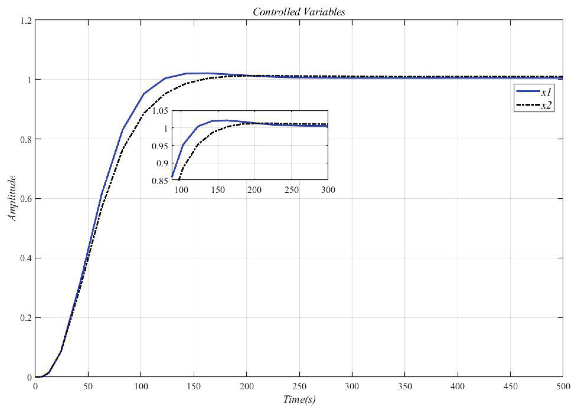
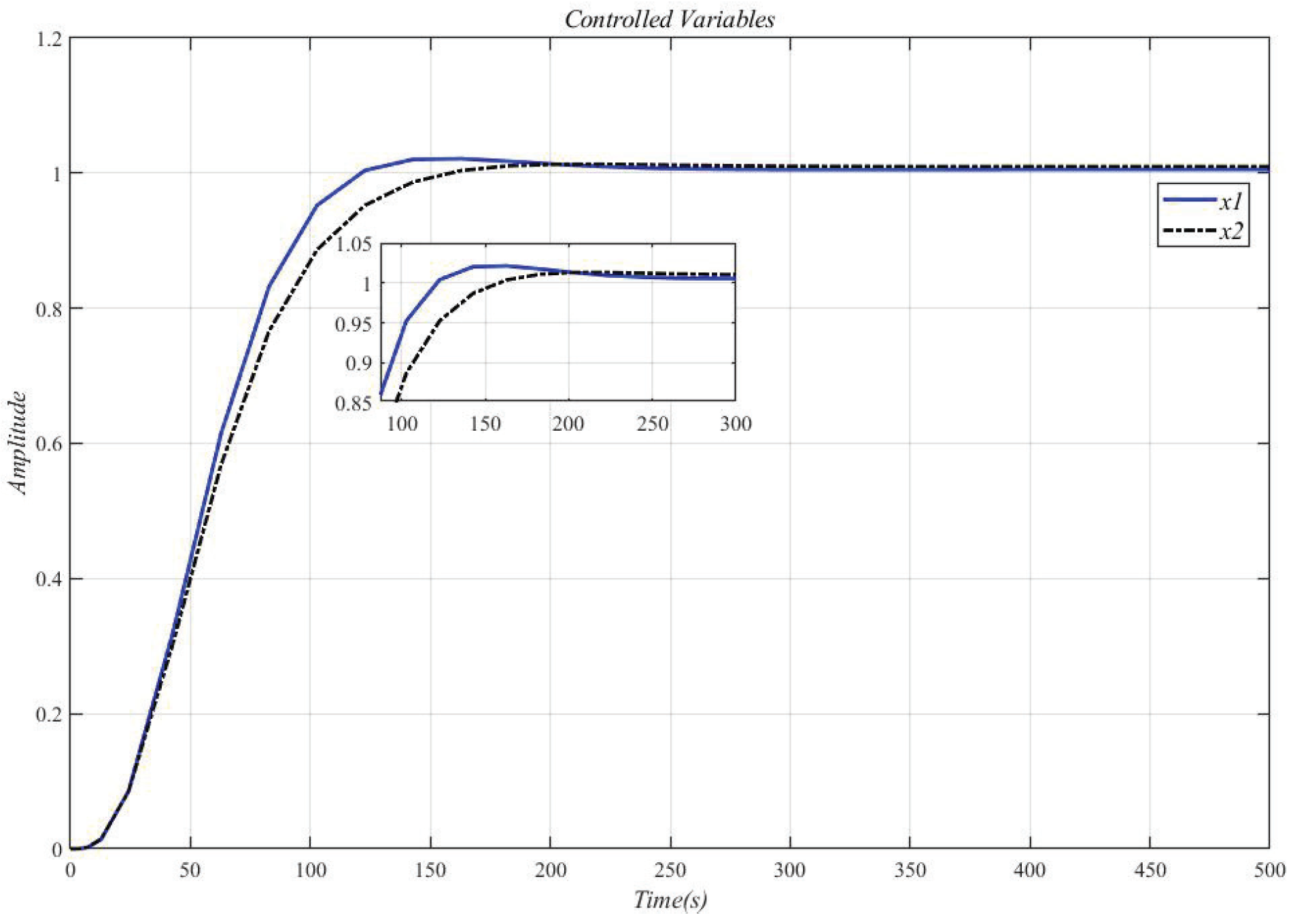
Using the CDM control polynomial parameters in
Table 8 to control
and
, the results are shown in
Figure 18.
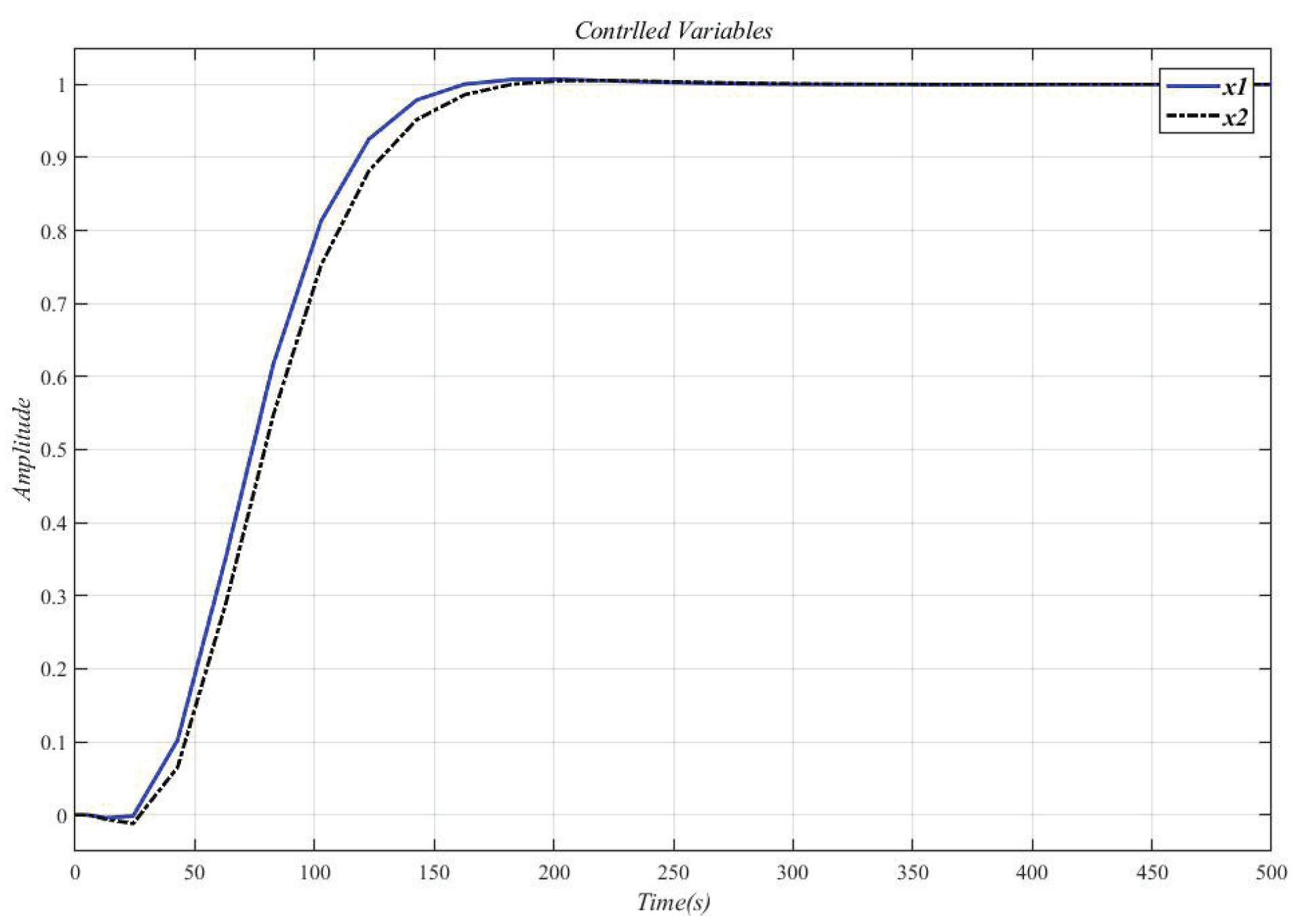
Figure 19 is the result of inserting the compensator (36) before the controlled object (35) and using the CDM parameters in
Table 8 for control.
Figure 18 is the same as
Figure 19, which proves that the decoupling effect is well.
Example 5. The controlled object (29) adds a line of input and a column output to become the controlled object (37). Using the method in this paper, select the angular frequency
, and obtain the compensator:
Use the evaluation (12) to evaluate the decoupling system
after the compensator formula (38) acts on the controlled object formula (37), and the result is 0.0005411. The two SISO systems after decoupling are set to
,
and
. For
,
and
, use the stability index
and
Table 9 equivalent time constant
to calculate the CDM control polynomial parameters.
Table 9 shows the equivalent time constant
and CDM control polynomial parameter values.
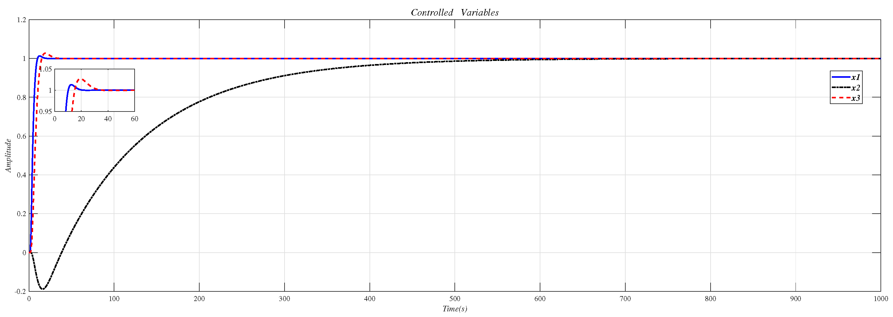
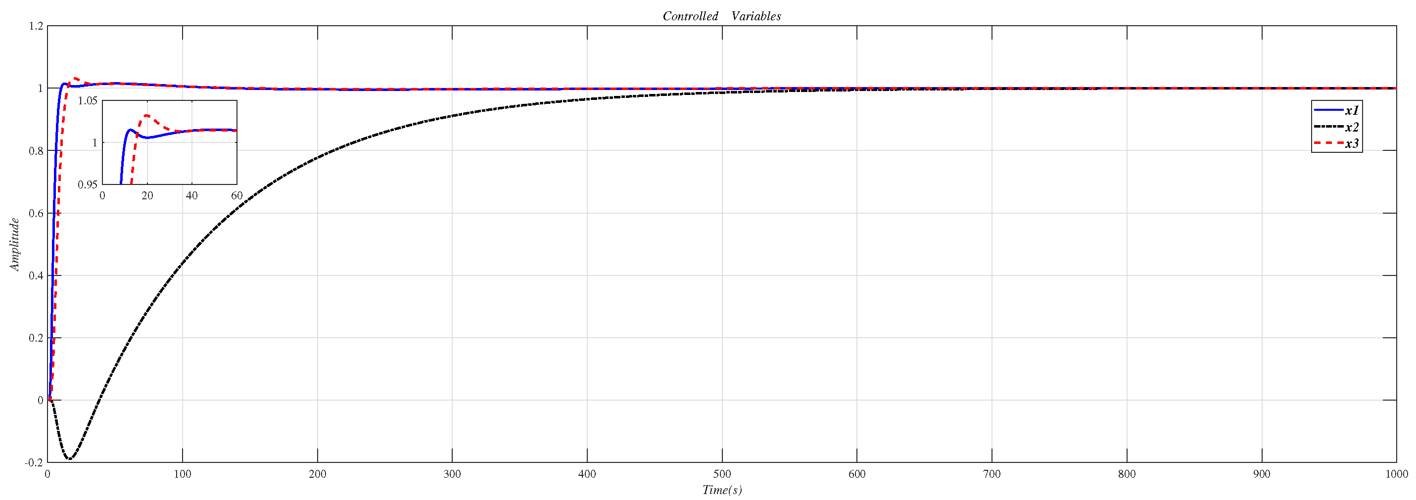
Using the CDM control polynomial parameters in
Table 9 to control
,
and
, the results are shown in
Figure 20.
Figure 21 is the result of inserting the compensator (38) before the controlled object (37) and using the CDM parameters in
Table 9 for control.


