
Ordinal Time Series Forecasting of the Air Quality Index


Abstract
:1. Introduction
2. Models and Methods
3. Data Collection
- (1)
- PRE or TEM with missing values: If PRE (TEM) is missing at day t, then we select the valid data of the nearest station to impute the missing value.
- (2)
- AQI with missing values: We use in the knn algorithm in terms of the smallest MAE and RMSE to impute the missing AQI value. We first identify the four days with PRE, TEM, WD, , and seasonal dummy values closest to the day with missing AQI, and the missing AQI is then substituted by the weighted average of the AQI values of these four days. The weights decrease as the distance of the case to its neighbor lengthens. We use a Gaussian kernel function to obtain the weights from the distances and refer for a detailed description of the distance to Torgo [21] on pages 61–62.
- (3)
- WD with missing values: We again use in the knn algorithm to impute the missing WD value. We first identify the four days with PRE, TEM, AQI, , and seasonal dummy values closest to the day with missing WD, and the missing WD is then substituted by the weighted average of the WD values of these four days.
4. Results
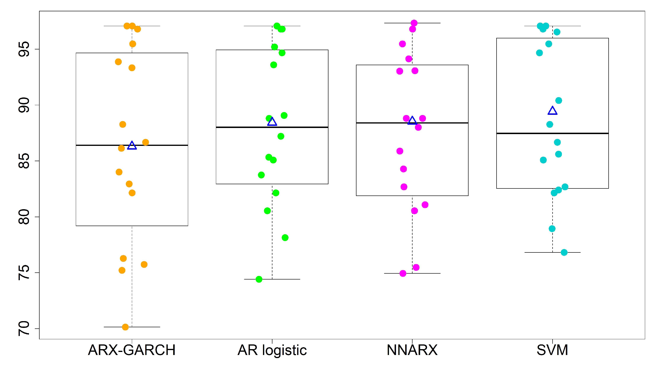
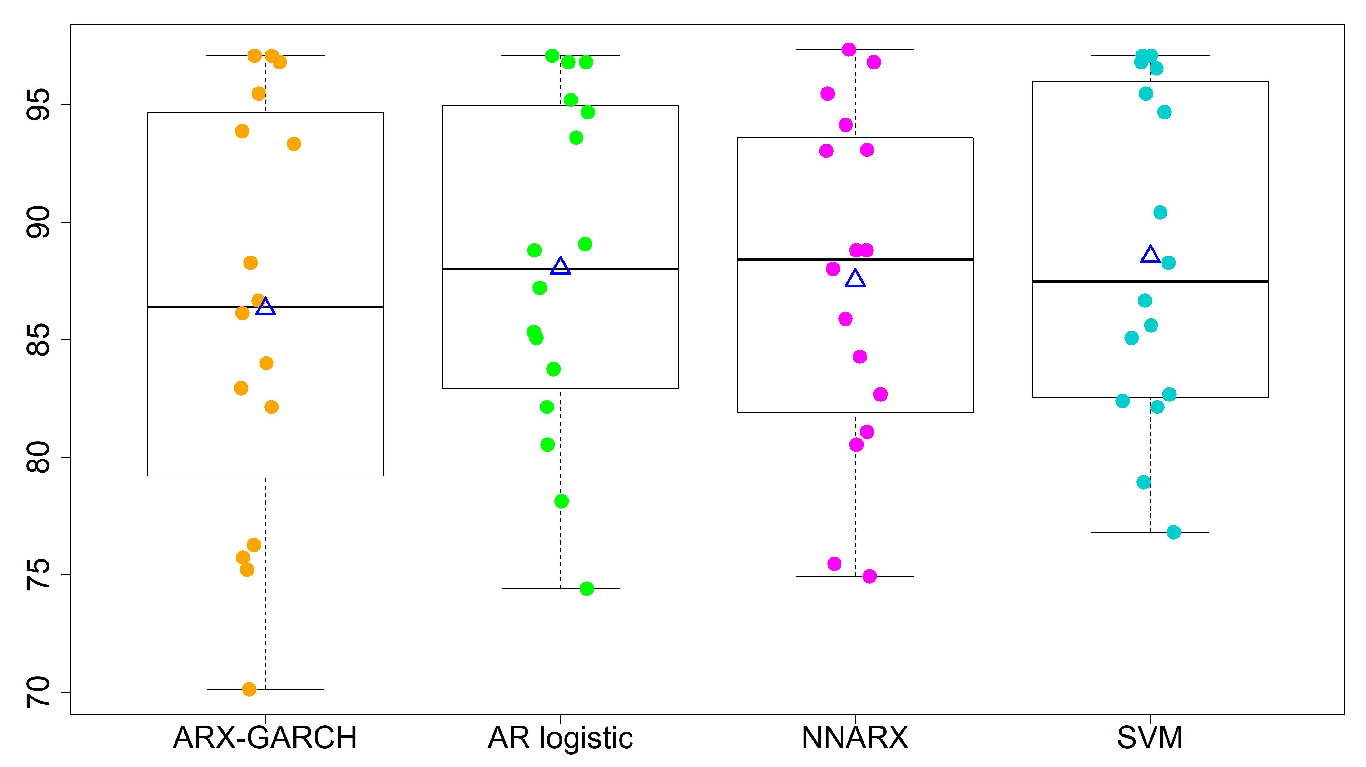
- The overall performances of the AR logistic regression, SVM, and NNARX are similar. Most accuracy rates by the three models are over 80%, except for sites 13 and 15. The SVM classification method has the highest average accuracy rate (88.53%) and the lowest standard deviation (7.00%) in the four-level predictions. The SVM method and AR logistic regression provide the lowest CV values among the four forecasting techniques. A lower CV is favored because it provides the most optimal forecasting performance with low variability, but a high average accuracy rate.
- The prediction performance is relatively low at sites 13 and 15, and so we need to scrutinize the time series data carefully. We perceive that the major misspecified levels occur in October. The three classification models (AR logistic regression, SVM, and NNARX) tend to misspecify the rare level.
- The lag-1 weather covariates of PRE and TEM with the hour-lag effect of WD are able to generate a reliable prediction level. We also consider wind speed and weekly/monthly weighted moving averages of AQI as extra covariates. However, these covariates do not improve forecast accuracy. Therefore, we do not include their results in the paper.
- The ARX-GARCH model is for quantitative forecasting purposes. The classification of wind directions in the sixteen sectors may not be suitable as an explanatory variable for this model.
5. Conclusions
Author Contributions
Funding
Institutional Review Board Statement
Informed Consent Statement
Data Availability Statement
Acknowledgments
Conflicts of Interest
Abbreviations
| AQI | Air quality index |
| AR logistic regression | Autoregressive multinomial logistic regression |
| ARX | Autoregression with exogenous variables |
| ARCH | Autoregressive conditional heteroskedasticity |
| GARCH | Generalized autoregressive conditional heteroskedasticity |
| NNARX | Neural network autoregression with exogenous variables |
| SVM | Support vector machine |
References
- Ferlito, S.; Bosso, F.; De Vito, S.; Esposito, E.; Di Francia, G. LSTM Networks for Particulate Matter Concentration Forecasting in AISEM Annual Conference on Sensors and Microsystems; Springer: Cham, Switzeland, 2019; pp. 409–415. [Google Scholar]
- Song, C.; Fu, X. Research on different weight combination in air quality forecasting models. J. Clean. Prod. 2020, 261, 121–169. [Google Scholar] [CrossRef]
- Wu, Q.; Lin, H. Daily urban air quality index forecasting based on variational mode decomposition, sample entropy and LSTM neural network. Sustain. Cities Soc. 2019, 50, 101–657. [Google Scholar] [CrossRef]
- Xiao, F.; Yang, M.; Fan, H.; Fan, G.; Al-Qaness, M.A. An improved deep learning model for predicting daily PM2.5 concentration. Sci. Rep. 2020, 10, 20988. [Google Scholar] [CrossRef] [PubMed]
- de Medrano, R.; Buen Remiro, V.; Aznarte, J.L. SOCAIRE: Forecasting and monitoring urban air quality in Madrid. Environ. Model. Softw. 2021, 143, 105084. [Google Scholar] [CrossRef]
- Liu, M.; Zhu, F.; Zhu, K. Modeling normalcy-dominant ordinal time series: An application to air quality level. J. Time Ser. Anal. 2021. [Google Scholar] [CrossRef]
- Kim, S.E. Ordinal time series model for forecasting air quality index for ozone in Southern California. Environ. Model. Assess. 2017, 22, 175–182. [Google Scholar] [CrossRef]
- Henry, R.C.; Chang, Y.; Spiegelman, C.H. Locating nearby sources of air pollution by nonparametric regression of atmospheric concentrations on wind direction. Atmos. Environ. 2002, 36, 2237–2244. [Google Scholar] [CrossRef]
- Carbajal-Hernàndez, J.J.; Sànchez-Fernàndez, L.P.; Carrasco-Ochoa, J.A.; Martìnez-Trinidad, J.F. Assessment and prediction of air quality using fuzzy logic and autoregressive models. Atmos. Environ. 2012, 60, 37–50. [Google Scholar] [CrossRef]
- So, M.K.P.; Chen, C.W.S.; Liu, F.C. Best subset selection of autoregressive models with exogenous variables and generalized autoregressive conditional heteroscedasticity errors. J. R. Stat. Soc. C Appl. Stat. 2006, 55, 201–224. [Google Scholar] [CrossRef]
- Chen, C.W.S.; Gerlach, R.; So, M.K.P. Bayesian model selection for heteroskedastic models. Bayesian Econom. 2008, 23, 567–594. [Google Scholar]
- Engle, R.F. Autoregressive conditional heteroscedasticity with estimates of the variance of United Kingdom inflation. Econometrica 1982, 50, 987–1007. [Google Scholar] [CrossRef]
- Bollerslev, T. Generalized autoregressive conditional heteroskedasticity. J. Econom. 1986, 31, 307–327. [Google Scholar] [CrossRef] [Green Version]
- Guanche, Y.; Minguez, R.; Méendez, F.J. Autoregressive logistic regression applied to atmospheric circulation patterns. Clim. Dyn. 2014, 42, 537–552. [Google Scholar] [CrossRef]
- Jiang, P.; Dong, Q.; Li, P. A novel hybrid strategy for PM2.5 concentration analysis and prediction. J. Environ. Manag. 2017, 196, 443–457. [Google Scholar] [CrossRef] [PubMed]
- Liu, B.C.; Binaykia, A.; Chang, P.C.; Tiwari, M.K.; Tsao, C.C. Urban air quality forecasting based on multi-dimensional collaborative support vector machines (SVM): A case study of Beijing-Tianjin-Shijiazhuang. PLoS ONE 2017, 12, e0179763. [Google Scholar]
- Liu, B.C.; Wang, H.; Binaykia, A.; Fu, C.C.; Xiang, B.P. Multi-level air quality classification in China using information gain and support vector machine hybrid model. Nat. Environ. Pollut. Technol. 2019, 18, 697–708. [Google Scholar]
- Hertz, J.A.; Krogh, A.S.; Palmer, R.G. Introduction to the Theory of Neural Computation; Westview Press: Boulder, CO, USA, 1991. [Google Scholar]
- Hyndman, R.J.; Athanasopoulos, G. Forecasting: Principles and Practice, 2rd ed.; OTexts: Melbourne, Australia, 2018. [Google Scholar]
- Cover, T.M.; Hart, P.E. Nearest neighbor pattern classification. IEEE Trans. Inf. Theory 1967, 13, 21–27. [Google Scholar] [CrossRef]
- Torgo, L. Data Mining with R, Learning with Case Studies; Chapman and Hall/CRC: Boca Raton, FL, USA, 2020. [Google Scholar]
- Hansen, B.E. Autoregressive conditional density estimation. J. Int. Econ. 1994, 35, 705–730. [Google Scholar] [CrossRef]
- Weiß, C.H. Distance-based analysis of ordinal data and ordinal time series. J. Am. Stat. Assoc. 2020, 115, 1189–1200. [Google Scholar] [CrossRef]
- Hsu, C.Y.; Chiang, H.C.; Lin, S.L.; Chen, M.J.; Lin, T.Y.; Chen, Y.C. Elemental characterization and source apportionment of PM10 and PM2.5 in the western coastal area of central Taiwan. Sci. Total Environ. 2016, 541, 1139–1150. [Google Scholar] [CrossRef]
- Chen, C.W.S.; Hsieh, Y.H.; Su, H.C.; Wu, J.J. Causality test of ambient fine particles and human influenza in Taiwan: Age group-specific disparity and geographic heterogeneity. Environ. Int. 2018, 111, 354–361. [Google Scholar] [CrossRef] [PubMed]
- Tseng, C.H.; Tsuang, B.J.; Chiang, C.J. et al. The relationship between air pollution and lung cancer in nonsmokers in Taiwan. J. Thorac. Oncol. 2019, 14, 784–792. [Google Scholar] [CrossRef] [PubMed]
- Tang, K.T.; Ku, K.C.; Chen, D.Y.; Lin, C.H.; Tsuang, B.J.; Chen, Y.H. Adult atopic dermatitis and exposure to air pollutants—A nationwide population-based study. Ann. Allergy Asthma Immunol. 2017, 118, 351–355. [Google Scholar] [CrossRef] [PubMed]
- Ghalanos, A.; Kley, T. Rugarch: Univariate GARCH Models; R Package Version 1.4-4; 2021; Available online: https://cran.r-project.org/web/packages/rugarch/index.html (accessed on 29 June 2021).
- Ripley, B.; Venables, B.; Bates, D.M.; Hornik, K. MASS: Support Functions and Datasets for Venables and Ripley’s MASS, R Package Version 7.3-54; 2021. Available online: http://www.stats.ox.ac.uk/pub/MASS4/ (accessed on 29 June 2021).
- Meyer, D.; Dimitriadou, E.; Hornik, K.; Weingessel, A.; Leisch, F. e1071: Misc Functions of the Department of Statistics, Probability Theory Group (Formerly: E1071), TU Wien, R Package Version 1.7-8; 2021. Available online: https://cran.r-project.org/web/packages/e1071/index.html (accessed on 29 June 2021).


| Value | Color | AQI Levels of Health Concern |
|---|---|---|
| 0–50 | Green | Good |
| 51–100 | Yellow | Satisfactory |
| 101–150 | Orange | Moderately |
| 151–200 | Red | Poor |
| 201–300 | Purple | Very poor |
| 301–500 | Maroon | Hazardous |
| Site | City/County | Mean | Std | Min | Max | ARCH Test (p-Value) |
|---|---|---|---|---|---|---|
| 1 | Shilin, Taipei | 54.888 | 23.799 | 13 | 185 | <0.0001 |
| 2 | Taoyuan, Taoyuan | 54.925 | 24.443 | 15 | 197 | <0.0001 |
| 3 | Dongqu, Hsinchu | 57.873 | 27.444 | 12 | 203 | <0.0001 |
| 4 | Miaoli, Miaoli | 61.197 | 25.893 | 13 | 172 | <0.0001 |
| 5 | Xitun, Taichung | 67.271 | 32.275 | 19 | 190 | <0.0001 |
| 6 | Fengyuan, Taichung | 62.861 | 29.702 | 15 | 207 | <0.0001 |
| 7 | Changhua, Changhua | 65.298 | 31.092 | 15 | 190 | <0.0001 |
| 8 | Douliu, Yunlin | 80.409 | 38.347 | 1 | 195 | <0.0001 |
| 9 | Xingang, Chiayi | 74.014 | 34.615 | 6 | 179 | <0.0001 |
| 10 | West, Chiayi | 75.400 | 36.941 | 16 | 179 | <0.0001 |
| 11 | West Central, Tainan | 74.512 | 37.539 | 17 | 195 | <0.0001 |
| 12 | Xinying, Tainan | 74.445 | 34.831 | 15 | 179 | <0.0001 |
| 13 | Zuoying, Kaohsiung | 81.031 | 42.767 | 17 | 210 | <0.0001 |
| 14 | Quian, Kaohsiung | 79.332 | 41.196 | 17 | 197 | <0.0001 |
| 15 | Pingtung, Pingtung | 81.964 | 39.995 | 15 | 206 | <0.0001 |
| 16 | Hengchun, Pingtung | 43.935 | 21.498 | 3 | 182 | <0.0001 |
| Category | Degree | Direction |
|---|---|---|
| 1 | 348.75–11.25 | N |
| 2 | 11.25–33.75 | NNE |
| 3 | 33.75–56.25 | NE |
| 4 | 56.25–78.75 | ENE |
| 5 | 78.75–101.25 | E |
| 6 | 101.25–123.75 | ESE |
| 7 | 123.75–146.25 | SE |
| 8 | 146.25–168.75 | SSE |
| 9 | 168.75–191.25 | S |
| 10 | 191.25–213.75 | SSW |
| 11 | 213.75–236.25 | SW |
| 12 | 236.25–258.75 | WSW |
| 13 | 258.75–281.25 | W |
| 14 | 281.25–303.75 | WNW |
| 15 | 303.75–326.25 | NW |
| 16 | 326.25–348.75 | NNW |
| Site | City/County | PRE | TEM | |||||
|---|---|---|---|---|---|---|---|---|
| Mean | Std | Max | Mean | Std | Min | Max | ||
| 1 | Shilin, Taipei | 4.70 | 14.40 | 202.0 | 23.94 | 5.32 | 8.10 | 33.10 |
| 2 | Taoyuan, Taoyuan | 5.02 | 15.28 | 175.0 | 22.25 | 5.56 | 6.90 | 32.40 |
| 3 | Dongqu, Hsinchu | 4.03 | 14.64 | 260.0 | 23.41 | 5.35 | 7.60 | 31.80 |
| 4 | Miaoli, Miaoli | 3.73 | 12.53 | 151.0 | 23.32 | 5.35 | 7.50 | 31.60 |
| 5 | Xitun, Taichung | 4.22 | 15.23 | 179.0 | 23.80 | 5.03 | 7.90 | 31.60 |
| 6 | Fengyuan, Taichung | 5.17 | 19.28 | 279.0 | 23.20 | 4.84 | 6.40 | 30.80 |
| 7 | Changhua, Changhua | 4.54 | 15.97 | 164.5 | 23.38 | 4.63 | 7.80 | 31.20 |
| 8 | Douliu, Yunlin | 4.67 | 19.41 | 415.0 | 23.70 | 4.64 | 8.20 | 31.30 |
| 9 | Xingang, Chiayi | 3.87 | 16.43 | 332.5 | 23.93 | 4.71 | 9.00 | 31.20 |
| 10 | West, Chiayi | 4.85 | 19.32 | 417.0 | 24.35 | 4.59 | 9.20 | 31.70 |
| 11 | West Central, Tainan | 5.00 | 21.71 | 373.0 | 24.97 | 4.44 | 9.70 | 31.60 |
| 12 | Xinying, Tainan | 4.62 | 20.50 | 451.5 | 24.33 | 4.57 | 9.00 | 31.50 |
| 13 | Zuoying, Kaohsiung | 4.62 | 19.24 | 283.5 | 24.97 | 4.03 | 10.20 | 30.90 |
| 14 | Qiangin, Kaohsiung | 5.06 | 21.02 | 291.5 | 25.32 | 3.85 | 10.90 | 30.30 |
| 15 | Pingtung, Pingtung | 6.44 | 24.92 | 357.0 | 25.14 | 3.57 | 11.00 | 31.20 |
| 16 | Hengchun, Pingtung | 5.42 | 20.18 | 326.0 | 25.91 | 3.12 | 15.50 | 31.00 |
| Site | City/County | Accuracy (%) | |||
|---|---|---|---|---|---|
| ARX-GARCH | AR Logistic | SVM | NNARX | ||
| 1 | Shilin, Taipei | 95.20 | 95.20 | 95.47 | 95.47 |
| 2 | Taoyuan, Taoyuan | 95.20 | 95.44 | 96.53 | 96.53 |
| 3 | Dongqu, Hsinchu | 93.60 | 93.16 | 97.07 | 93.07 |
| 4 | Miaoli, Miaoli | 96.00 | 96.71 | 96.80 | 97.33 |
| 5 | Xitun, Taichung | 86.13 | 87.85 | 90.93 | 89.07 |
| 6 | Fengyuan, Taichung | 88.53 | 89.62 | 88.27 | 89.07 |
| 7 | Changhua, Changhua | 91.73 | 91.20 | 94.67 | 94.13 |
| 8 | Douliu, Yunlin | 78.13 | 81.52 | 84.27 | 82.93 |
| 9 | Xingang, Chiayi | 83.47 | 86.58 | 85.60 | 84.27 |
| 10 | West, Chiayi | 81.87 | 85.32 | 85.60 | 88.27 |
| 11 | West Central, Tainan | 80.53 | 83.04 | 83.20 | 82.93 |
| 12 | Xinying, Tainan | 84.00 | 87.85 | 87.20 | 86.13 |
| 13 | Zuoying, Kaohsiung | 78.93 | 82.67 | 81.60 | 79.73 |
| 14 | Qianjin, Kaohsiung | 76.80 | 82.40 | 83.47 | 82.13 |
| 15 | Pingtung, Pingtung | 73.07 | 78.13 | 82.93 | 78.40 |
| 16 | Hengchun, Pingtung | 97.60 | 98.23 | 97.07 | 97.07 |
| Site | City/County | Accuracy (%) | |||
|---|---|---|---|---|---|
| ARX-GARCH | AR Logistic | SVM | NNARX | ||
| 1 | Shilin, Taipei | 95.47 | 95.20 | 95.47 | 95.47 |
| 2 | Taoyuan, Taoyuan | 96.80 | 96.80 | 96.53 | 93.03 |
| 3 | Dongqu, Hsinchu | 93.33 | 93.60 | 97.07 | 93.07 |
| 4 | Miaoli, Miaoli | 97.07 | 97.07 | 96.80 | 97.33 |
| 5 | Xitun, Taichung | 86.67 | 89.07 | 90.40 | 88.80 |
| 6 | Fengyuan, Taichung | 88.27 | 88.80 | 88.27 | 88.80 |
| 7 | Changhua, Changhua | 93.87 | 94.67 | 94.67 | 94.13 |
| 8 | Douliu, Yunlin | 76.27 | 82.13 | 82.13 | 81.07 |
| 9 | Xingang, Chiayi | 84.00 | 85.07 | 85.60 | 84.27 |
| 10 | West, Chiayi | 82.93 | 85.33 | 85.07 | 88.00 |
| 11 | West Central, Tainan | 82.13 | 83.73 | 82.67 | 82.67 |
| 12 | Xinying, Tainan | 86.13 | 87.20 | 86.67 | 85.87 |
| 13 | Zuoying, Kaohsiung | 75.73 | 78.13 | 76.80 | 75.47 |
| 14 | Qianjin, Kaohsiung | 75.20 | 80.53 | 82.40 | 80.53 |
| 15 | Pingtung, Pingtung | 70.13 | 74.40 | 78.93 | 74.93 |
| 16 | Hengchun, Pingtung | 97.07 | 96.80 | 97.07 | 96.80 |
| Average (%) | 86.32 | 88.03 | 88.53 | 87.52 | |
| Std (%) | 8.825 | 7.182 | 7.000 | 7.234 | |
| CV | 0.1022 | 0.0816 | 0.0790 | 0.0826 | |
Publisher’s Note: MDPI stays neutral with regard to jurisdictional claims in published maps and institutional affiliations. |
© 2021 by the authors. Licensee MDPI, Basel, Switzerland. This article is an open access article distributed under the terms and conditions of the Creative Commons Attribution (CC BY) license (https://creativecommons.org/licenses/by/4.0/).
Share and Cite
Chen, C.W.S.; Chiu, L.M. Ordinal Time Series Forecasting of the Air Quality Index. Entropy 2021, 23, 1167. https://doi.org/10.3390/e23091167
Chen CWS, Chiu LM. Ordinal Time Series Forecasting of the Air Quality Index. Entropy. 2021; 23(9):1167. https://doi.org/10.3390/e23091167
Chicago/Turabian StyleChen, Cathy W. S., and L. M. Chiu. 2021. "Ordinal Time Series Forecasting of the Air Quality Index" Entropy 23, no. 9: 1167. https://doi.org/10.3390/e23091167
APA StyleChen, C. W. S., & Chiu, L. M. (2021). Ordinal Time Series Forecasting of the Air Quality Index. Entropy, 23(9), 1167. https://doi.org/10.3390/e23091167