
Quantum Heat Engines with Complex Working Media, Complete Otto Cycles and Heuristics


Abstract
:1. Introduction
2. Quantum Otto Cycle
2.1. The Heat Cycle
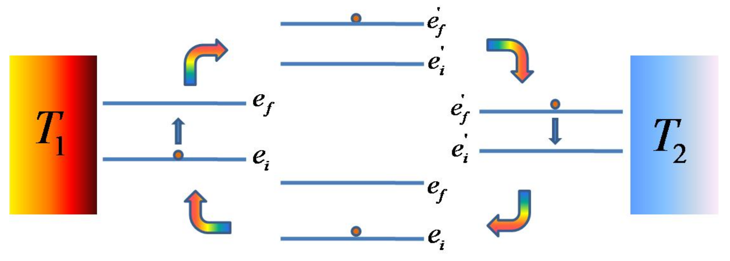
- Stage 1:
- The system is at thermal equilibrium with a heat reservoir at temperature with energy for which its occupation probabilities are , and the corresponding density matrix is (here, we are considering two non interacting spins with energy eigenvalues denoted by and occupation probabilities by ).
- Stage 2:
- The system undergoes a quantum adiabatic process after it is isolated from the hot bath, and the magnetic field is changed from to a smaller value . Here, the quantum adiabatic theorem is assumed to hold according to which the process should be slow enough so that no transitions are induced as the energy levels change from to .
- Stage 3:
- Here, the system is brought in contact with a cold bath at temperature (<). The energy eigenvalues remain at , and the occupation probabilities change from to with the external magnetic field at , and the density matrix of the system is .
- Stage 4:
- The system is detached from the cold bath, and the magnetic field is changed from to with occupation probabilities remaining unchanged at and energy eigenvalues changing back from to such that only work is performed on the system during this step. Finally, the system is attached to the hot bath again, and the cycle is completed such that the average heat absorbed is , and the net work performed per cycle is . Here, denotes the trace operation, and . In this paper, we consider the free Hamiltonian of the form (), where is an operator. We now have ; therefore, the efficiency in the absence of interaction is as follows.
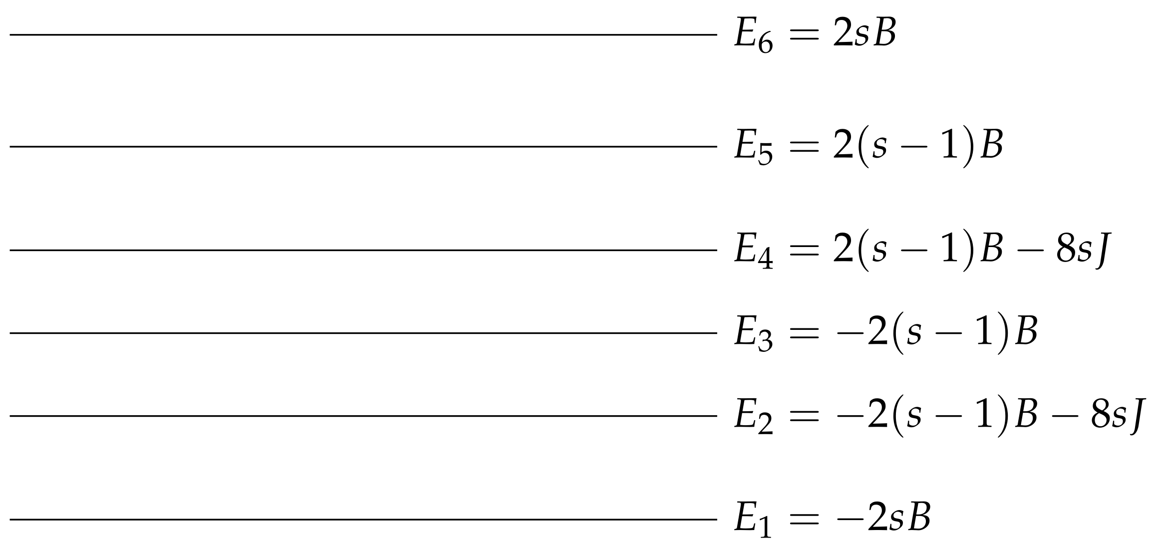
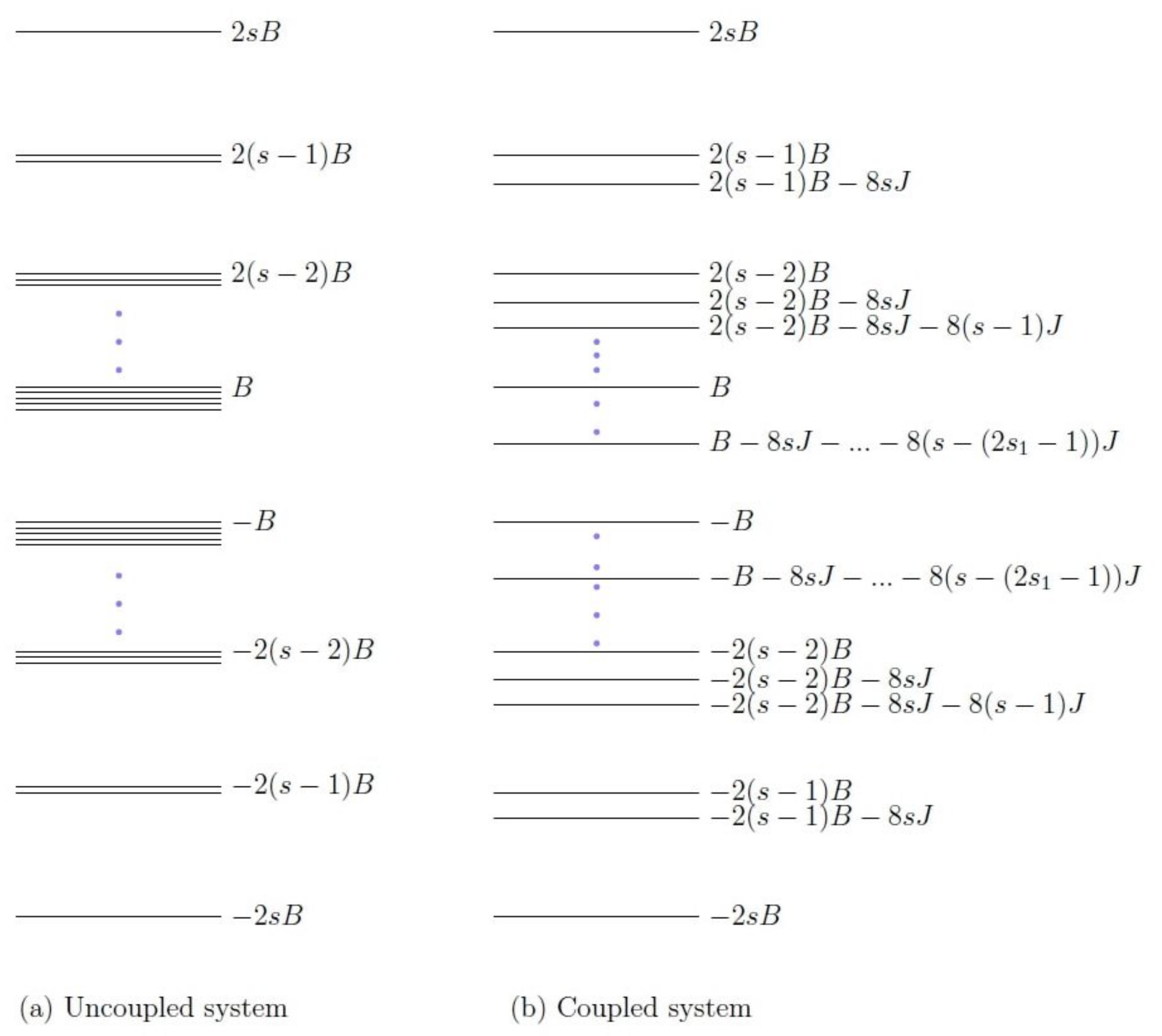
3. The Coupled Model
3.1. Majorization
3.2. Energy Level Ordering
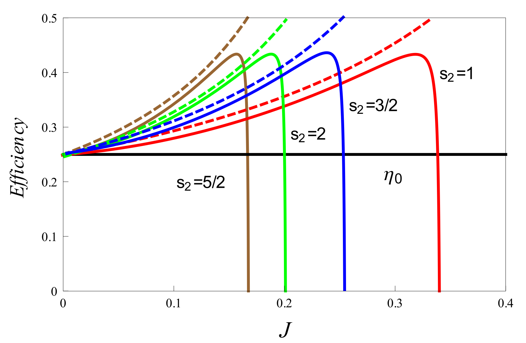
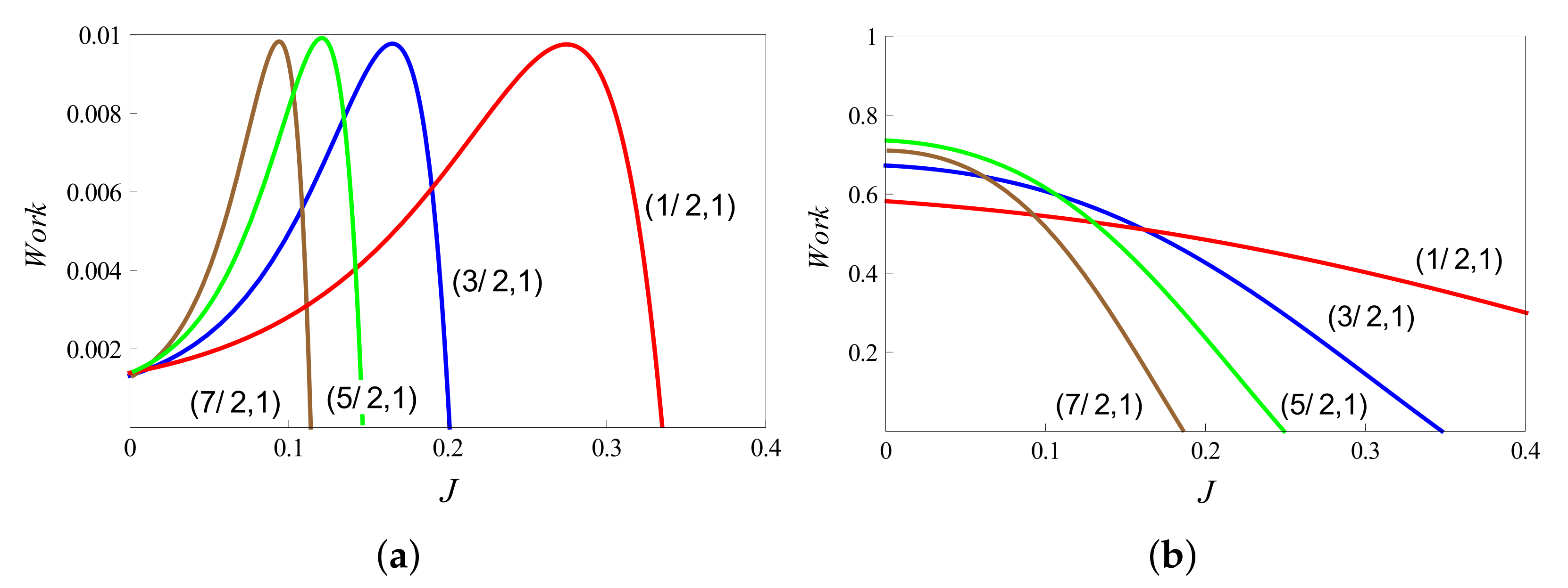
4. Efficiency Enhancement and the Upper Bound
- When one spin value is a half-integer and the other is an integer;
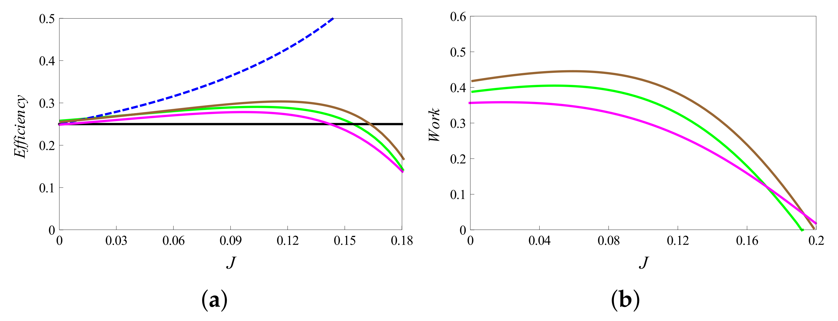
- When both values are half-integer or both are integers;
- When both are of the same magnitude (both as half-integer or integer).
5. Complete Otto Cycles
- : These cycles occur between any two different energy bands having the same . Therefore, if such a cycle proceeds as an engine (), its efficiency is . From Equation (24), this COC is consistent with the second law for .
- : These cycles are possible between energy levels of the same band, i.e., having same . The work performed is zero, and the heat exchanged is . Thus, for , the corresponding efficiency is also zero.
- with the same sign: These cycles are possible between different bands for levels with different and . If such cycles proceed as engine, i.e., (and ), then the corresponding efficiency is the following.From Equation (24), this type of COC is consistent with the second law for , without imposing any further condition on the coupling strength . Therefore, if the second law allows COCs with , then it also allows COCs with .
- with opposite signs: These cycles occur between energy levels of different bands with different and . If for such cycles (and ), the corresponding efficiency is as follows.
6. Discussion
Author Contributions
Funding
Institutional Review Board Statement
Informed Consent Statement
Data Availability Statement
Conflicts of Interest
Appendix A. PWC for the Coupled Model
Appendix B. PWC for the Coupled Model

| . |
| . |
| . |
| . |
| . |
| . |
| . |
| . |
| . |
| . |
| . |
| . |
- (a)
- , which implies the following:
- 1
- ;
- 2
- , thereby proving that under , it is not possible for the coupled system to work as an engine at all.
- (b)
- , which implies the following:
- 1
- does not bear a definite sign. Although the term () in is positive definite, yet the sign of the other term () is not definite;
- 2
- Under WCS, we are able to prove for , thereby implying that it is a necessary condition for . However, WCS also demands or . Therefore, the latter constitutes a sufficient condition for .
- 3
- When does not hold, does not have definite sign. Thus, depending on the control parameters, other terms in X can be positive. In this case, we cannot predict the sign of .
- a
- If (which happens for ), then .
- b
- If (which happens for and ), then .
- c
- If no definite sign can be assigned to (which may happen even when holds, but with no condition on the range of J), the system may or may not work as an engine.
Appendix C. Condition on J from Wav > 0
| k | ||
|---|---|---|
| 0 | 1 | |
| . | . | . |
| . | . | . |
| . | . | . |
| . | . | . |
| 0 | n |
Appendix D. Proof for X > Y1
- We first consider the lower half levels. With being negative for all (see Table A2), the total contribution from these levels to X takes the following form.Similarly, the coefficients of these terms in can be calculated from Table A2 as (note that holds for all k).Now, we add these to obtain the coefficients of these terms in U, denoted by , which have been listed in Table A3. As can be observed, has a positive part given by "s" and a negative part, say . The total contribution from the lower half levels to U is therefore written as follows.With , the second part is positive because of Equation (A29), and the first part is considered later on.
| k | |
|---|---|
| 1 | s |
| . | . |
| . | . |
- 2.
- We now consider the upper half levels. The total contribution of these levels to X and is considered separately. The former is given as the following.With being positive (Table A2) for all , the above expression is positive because of Equation (A29).As for these levels’ contribution to , it is given as the following.
| k | ||
|---|---|---|
| . | . | |
| . | . | |
| n | 0 | 0 |
- 3.
- Adding up the total contribution to U from all the energy levels we have the following.From the first and second points, we now have two parts which are yet to be proved positive. Their sum is given as follows.Using relations such as and (from Equation (A29)) and in the normalization condition of the following probabilities:we have the following.As shown below, . Therefore, with , we can safely replace s by in the above inequality, thereby proving .
Proof for m5 < s
| k | ||
|---|---|---|
| 0 | 1 | |
| 0 | 6 |
- We first consider the lower half () of the levels. With being negative (see Table A5), the total contribution from these levels to X takes the form of the following.Similarly, contribution of lower half levels to is written as follows.The total contribution of the lower half levels to U is as follows.The second part is positive because of Equation (A29), and the first part is considered later on.
- We now consider the upper half levels. The total contribution of these levels to X and is considered separately. The former is given as follows.The above expression is positive because of Equation (A29).As for these levels’ contribution to , it is given as the following.This part is negative and will be considered later on.
- From points one and two the following terms in U are yet to be shown positive.Using relations such , (from Equation (A29)) and in the normalization condition of probabilities, given as the following:we have the following.With and ( for the present case), we can safely replace s by 1 in the the above expression, thereby proving .
References
- Gemmer, J.; Michel, M.; Mahler, G. Quantum Thermodynamics: Emergence of Thermodynamic Behavior within Composite Quantum Systems; Springer: Berlin/Heidelberg, Germany, 2009; Volume 784. [Google Scholar]
- Kosloff, R. Quantum thermodynamics: A dynamical viewpoint. Entropy 2013, 15, 2100–2128. [Google Scholar] [CrossRef] [Green Version]
- Binder, F.; Correa, L.A.; Gogolin, C.; Anders, J.; Adesso, G. Thermodynamics in the quantum regime. Fundam. Theor. Phys. 2018, 195. [Google Scholar] [CrossRef]
- Quan, H.T.; Liu, Y.X.; Sun, C.P.; Nori, F. Quantum thermodynamic cycles and quantum heat engines. Phys. Rev. E 2007, 76, 031105. [Google Scholar] [CrossRef] [Green Version]
- Allahverdyan, A.E.; Johal, R.S.; Mahler, G. Work extremum principle: Structure and function of quantum heat engines. Phys. Rev. E 2008, 77, 041118. [Google Scholar] [CrossRef] [PubMed] [Green Version]
- Thomas, G.; Johal, R.S. Coupled quantum Otto cycle. Phys. Rev. E 2011, 83, 031135. [Google Scholar] [CrossRef] [Green Version]
- Esposito, M.; Kumar, N.; Lindenberg, K.; Van den Broeck, C. Stochastically driven single-level quantum dot: A nanoscale finite-time thermodynamic machine and its various operational modes. Phys. Rev. E 2012, 85, 031117. [Google Scholar] [CrossRef] [PubMed] [Green Version]
- Kolář, M.; Gelbwaser-Klimovsky, D.; Alicki, R.; Kurizki, G. Quantum bath refrigeration towards absolute zero: Challenging the unattainability principle. Phys. Rev. Lett. 2012, 109, 090601. [Google Scholar] [CrossRef] [Green Version]
- Levy, A.; Kosloff, R. Quantum absorption refrigerator. Phys. Rev. Lett. 2012, 108, 070604. [Google Scholar] [CrossRef] [PubMed] [Green Version]
- Hewgill, A.; Ferraro, A.; De Chiara, G. Quantum correlations and thermodynamic performances of two-qubit engines with local and common baths. Phys. Rev. A 2018, 98, 042102. [Google Scholar] [CrossRef] [Green Version]
- Agarwal, G.S.; Chaturvedi, S. Quantum dynamical framework for Brownian heat engines. Phys. Rev. E 2013, 88, 012130. [Google Scholar] [CrossRef] [PubMed] [Green Version]
- Correa, L.A.; Palao, J.P.; Adesso, G.; Alonso, D. Performance bound for quantum absorption refrigerators. Phys. Rev. E 2013, 87, 042131. [Google Scholar] [CrossRef] [Green Version]
- Del Campo, A.; Goold, J.; Paternostro, M. More bang for your buck: Super-adiabatic quantum engines. Sci. Rep. 2014, 4, 1–5. [Google Scholar]
- Gelbwaser-Klimovsky, D.; Alicki, R.; Kurizki, G. Minimal universal quantum heat machine. Phys. Rev. E 2013, 87, 012140. [Google Scholar] [CrossRef] [PubMed] [Green Version]
- Venturelli, D.; Fazio, R.; Giovannetti, V. Minimal self-contained quantum refrigeration machine based on four quantum dots. Phys. Rev. Lett. 2013, 110, 256801. [Google Scholar] [CrossRef] [Green Version]
- Long, R.; Liu, W. Performance of quantum Otto refrigerators with squeezing. Phys. Rev. E 2015, 91, 062137. [Google Scholar] [CrossRef] [PubMed]
- Ou, C.; Abe, S. Exotic properties and optimal control of quantum heat engine. EPL (Europhys. Lett.) 2016, 113, 40009. [Google Scholar] [CrossRef] [Green Version]
- Mehta, V.; Johal, R.S. Quantum Otto engine with exchange coupling in the presence of level degeneracy. Phys. Rev. E 2017, 96, 032110. [Google Scholar] [CrossRef] [Green Version]
- Erdman, P.A.; Mazza, F.; Bosisio, R.; Benenti, G.; Fazio, R.; Taddei, F. Thermoelectric properties of an interacting quantum dot based heat engine. Phys. Rev. B 2017, 95, 245432. [Google Scholar] [CrossRef] [Green Version]
- Watanabe, G.; Venkatesh, B.P.; Talkner, P.; del Campo, A. Quantum Performance of Thermal Machines over Many Cycles. Phys. Rev. Lett. 2017, 118, 050601. [Google Scholar] [CrossRef] [Green Version]
- Chand, S.; Biswas, A. Measurement-induced operation of two-ion quantum heat machines. Phys. Rev. E 2017, 95, 032111. [Google Scholar] [CrossRef] [Green Version]
- Agarwalla, B.K.; Jiang, J.H.; Segal, D. Quantum efficiency bound for continuous heat engines coupled to noncanonical reservoirs. Phys. Rev. B 2017, 96, 104304. [Google Scholar] [CrossRef] [Green Version]
- Niedenzu, W.; Mukherjee, V.; Ghosh, A.; Kofman, A.G.; Kurizki, G. Quantum engine efficiency bound beyond the second law of thermodynamics. Nat. Commun. 2018, 9, 1–13. [Google Scholar] [CrossRef] [Green Version]
- Zhang, K.; Zhang, W. Quantum optomechanical straight-twin engine. Phys. Rev. A 2017, 95, 053870. [Google Scholar] [CrossRef] [Green Version]
- Türkpençe, D.; Altintas, F. Coupled quantum Otto heat engine and refrigerator with inner friction. Quantum Inf. Process. 2019, 18, 255. [Google Scholar] [CrossRef]
- Çakmak, B.; Müstecaplıoğlu, Ö.E. Spin quantum heat engines with shortcuts to adiabaticity. Phys. Rev. E 2019, 99, 032108. [Google Scholar] [CrossRef] [PubMed] [Green Version]
- Xu, H.; Yung, M.H. Unruh quantum Otto heat engine with level degeneracy. Phys. Lett. B 2020, 801, 135201. [Google Scholar] [CrossRef]
- de Assis, R.J.; Sales, J.S.; Mendes, U.C.; de Almeida, N.G. Two-level quantum Otto heat engine operating with unit efficiency far from the quasi-static regime under a squeezed reservoir. J. Phys. B At. Mol. Opt. Phys. 2021, 54, 095501. [Google Scholar] [CrossRef]
- Huang, X.; Yang, A.; Zhang, H.; Zhao, S.; Wu, S. Two particles in measurement-based quantum heat engine without feedback control. Quantum Inf. Process. 2020, 19, 1–14. [Google Scholar] [CrossRef]
- Zhang, Y. Optimization performance of quantum Otto heat engines and refrigerators with squeezed thermal reservoirs. Phys. A Stat. Mech. Its Appl. 2020, 559, 125083. [Google Scholar] [CrossRef]
- Lee, S.; Ha, M.; Park, J.M.; Jeong, H. Finite-time quantum Otto engine: Surpassing the quasistatic efficiency due to friction. Phys. Rev. E 2020, 101, 022127. [Google Scholar] [CrossRef] [PubMed] [Green Version]
- Chand, S.; Biswas, A. Critical-point behavior of a measurement-based quantum heat engine. Phys. Rev. E 2018, 98, 052147. [Google Scholar] [CrossRef] [Green Version]
- Hong, Y.; Xiao, Y.; He, J.; Wang, J. Quantum Otto engine working with interacting spin systems: Finite power performance in stochastic thermodynamics. Phys. Rev. E 2020, 102, 022143. [Google Scholar] [CrossRef]
- Dey, A.; Bhakuni, D.S.; Agarwalla, B.K.; Sharma, A. Quantum entanglement and transport in a non-equilibrium interacting double-dot system: The curious role of degeneracy. J. Phys. Condens. Matter 2019, 32, 075603. [Google Scholar] [CrossRef] [Green Version]
- Latune, C.L.; Sinayskiy, I.; Petruccione, F. Apparent temperature: Demystifying the relation between quantum coherence, correlations, and heat flows. Quantum Sci. Technol. 2019, 4, 025005. [Google Scholar] [CrossRef] [Green Version]
- Halpern, N.Y.; White, C.D.; Gopalakrishnan, S.; Refael, G. Quantum engine based on many-body localization. Phys. Rev. B 2019, 99, 024203. [Google Scholar] [CrossRef] [Green Version]
- de Assis, R.J.; de Mendonça, T.M.; Villas-Boas, C.J.; de Souza, A.M.; Sarthour, R.S.; Oliveira, I.S.; de Almeida, N.G. Efficiency of a quantum Otto heat engine operating under a reservoir at effective negative temperatures. Phys. Rev. Lett. 2019, 122, 240602. [Google Scholar] [CrossRef] [PubMed] [Green Version]
- Park, J.M.; Lee, S.; Chun, H.M.; Noh, J.D. Quantum mechanical bound for efficiency of quantum Otto heat engine. Phys. Rev. E 2019, 100, 012148. [Google Scholar] [CrossRef] [Green Version]
- Johnson, C.V. Holographic heat engines as quantum heat engines. Class. Quantum Gravity 2020, 37, 034001. [Google Scholar] [CrossRef] [Green Version]
- Abiuso, P.; Miller, H.J.; Perarnau-Llobet, M.; Scandi, M. Geometric optimisation of quantum thermodynamic processes. Entropy 2020, 22, 1076. [Google Scholar] [CrossRef]
- Abah, O.; Paternostro, M.; Lutz, E. Shortcut-to-adiabaticity quantum Otto refrigerator. Phys. Rev. Res. 2020, 2, 023120. [Google Scholar] [CrossRef]
- Singh, V.; Pandit, T.; Johal, R.S. Optimal performance of a three-level quantum refrigerator. Phys. Rev. E 2020, 101, 062121. [Google Scholar] [CrossRef]
- Myers, N.M.; Deffner, S. Bosons outperform fermions: The thermodynamic advantage of symmetry. Phys. Rev. E 2020, 101, 012110. [Google Scholar] [CrossRef] [Green Version]
- Wang, Q. Performance of quantum heat engines under the influence of long-range interactions. Phys. Rev. E 2020, 102, 012138. [Google Scholar] [CrossRef]
- Makarov, D.N. Quantum entanglement and reflection coefficient for coupled harmonic oscillators. Phys. Rev. E 2020, 102, 052213. [Google Scholar] [CrossRef]
- Peña, F.J.; Zambrano, D.; Negrete, O.; De Chiara, G.; Orellana, P.A.; Vargas, P. Quasistatic and quantum-adiabatic Otto engine for a two-dimensional material: The case of a graphene quantum dot. Phys. Rev. E 2020, 101, 012116. [Google Scholar] [CrossRef] [PubMed] [Green Version]
- Shirai, Y.; Hashimoto, K.; Tezuka, R.; Uchiyama, C.; Hatano, N. Non-Markovian effect on quantum Otto engine: Role of system-reservoir interaction. Phys. Rev. Res. 2021, 3, 023078. [Google Scholar] [CrossRef]
- Camati, P.A.; Santos, J.F.G.; Serra, R.M. Employing non-Markovian effects to improve the performance of a quantum Otto refrigerator. Phys. Rev. A 2020, 102, 012217. [Google Scholar] [CrossRef]
- Gelbwaser-Klimovsky, D.; Kopylov, W.; Schaller, G. Cooperative efficiency boost for quantum heat engines. Phys. Rev. A 2019, 99, 022129. [Google Scholar] [CrossRef] [Green Version]
- Jiao, G.; Zhu, S.; He, J.; Ma, Y.; Wang, J. Fluctuations in irreversible quantum Otto engines. Phys. Rev. E 2021, 103, 032130. [Google Scholar] [CrossRef] [PubMed]
- Adesso, G.; Ragy, S.; Lee, A.R. Continuous variable quantum information: Gaussian states and beyond. Open Syst. Inf. Dyn. 2014, 21, 1440001. [Google Scholar] [CrossRef] [Green Version]
- Scappucci, G.; Kloeffel, C.; Zwanenburg, F.A.; Loss, D.; Myronov, M.; Zhang, J.J.; De Franceschi, S.; Katsaros, G.; Veldhorst, M. The germanium quantum information route. Nat. Rev. Mater. 2020, 1–18. [Google Scholar] [CrossRef]
- Goold, J.; Huber, M.; Riera, A.; Del Rio, L.; Skrzypczyk, P. The role of quantum information in thermodynamics—A topical Rev. J. Phys. A Math. Theor. 2016, 49, 143001. [Google Scholar] [CrossRef]
- Liu, X.; Hersam, M.C. 2D materials for quantum information science. Nat. Rev. Mater. 2019, 4, 669–684. [Google Scholar] [CrossRef]
- Roßnagel, J.; Dawkins, S.T.; Tolazzi, K.N.; Abah, O.; Lutz, E.; Schmidt-Kaler, F.; Singer, K. A single-atom heat engine. Science 2016, 352, 325–329. [Google Scholar] [CrossRef] [PubMed] [Green Version]
- Maslennikov, G.; Ding, S.; Hablützel, R.; Gan, J.; Roulet, A.; Nimmrichter, S.; Dai, J.; Scarani, V.; Matsukevich, D. Quantum absorption refrigerator with trapped ions. Nat. Commun. 2019, 10, 1–8. [Google Scholar] [CrossRef] [PubMed]
- Ono, K.; Shevchenko, S.; Mori, T.; Moriyama, S.; Nori, F. Analog of a quantum heat engine using a single-spin qubit. Phys. Rev. Lett. 2020, 125, 166802. [Google Scholar] [CrossRef]
- Cimini, V.; Gherardini, S.; Barbieri, M.; Gianani, I.; Sbroscia, M.; Buffoni, L.; Paternostro, M.; Caruso, F. Experimental characterization of the energetics of quantum logic gates. NPJ Quantum Inf. 2020, 6, 1–8. [Google Scholar] [CrossRef]
- Benenti, G.; Casati, G.; Saito, K.; Whitney, R.S. Fundamental aspects of steady-state conversion of heat to work at the nanoscale. Phys. Rep. 2017, 694, 1–124. [Google Scholar] [CrossRef] [Green Version]
- Gelbwaser-Klimovsky, D.; Niedenzu, W.; Kurizki, G. Thermodynamics of quantum systems under dynamical control. In Advances In Atomic, Molecular, and Optical Physics; Elsevier: Amsterdam, The Netherlands, 2015; Volume 64, pp. 329–407. [Google Scholar]
- Roßnagel, J.; Abah, O.; Schmidt-Kaler, F.; Singer, K.; Lutz, E. Nanoscale heat engine beyond the Carnot limit. Phys. Rev. Lett. 2014, 112, 030602. [Google Scholar] [CrossRef]
- Gelbwaser-Klimovsky, D.; Bylinskii, A.; Gangloff, D.; Islam, R.; Aspuru-Guzik, A.; Vuletic, V. Single-atom heat machines enabled by energy quantization. Phys. Rev. Lett. 2018, 120, 170601. [Google Scholar] [CrossRef] [Green Version]
- Zheng, Y.; Poletti, D. Quantum statistics and the performance of engine cycles. Phys. Rev. E 2015, 92, 012110. [Google Scholar] [CrossRef] [Green Version]
- Brantut, J.P.; Grenier, C.; Meineke, J.; Stadler, D.; Krinner, S.; Kollath, C.; Esslinger, T.; Georges, A. A thermoelectric heat engine with ultracold atoms. Science 2013, 342, 713–715. [Google Scholar] [CrossRef] [PubMed] [Green Version]
- Roulet, A.; Nimmrichter, S.; Arrazola, J.M.; Seah, S.; Scarani, V. Autonomous rotor heat engine. Phys. Rev. E 2017, 95, 062131. [Google Scholar] [CrossRef] [Green Version]
- Cherubim, C.; Brito, F.; Deffner, S. Non-thermal quantum engine in transmon qubits. Entropy 2019, 21, 545. [Google Scholar] [CrossRef] [PubMed] [Green Version]
- Peterson, J.P.; Batalhão, T.B.; Herrera, M.; Souza, A.M.; Sarthour, R.S.; Oliveira, I.S.; Serra, R.M. Experimental characterization of a spin quantum heat engine. Phys. Rev. Lett. 2019, 123, 240601. [Google Scholar] [CrossRef] [Green Version]
- Van Horne, N.; Yum, D.; Dutta, T.; Hänggi, P.; Gong, J.; Poletti, D.; Mukherjee, M. Single-atom energy-conversion device with a quantum load. NPJ Quantum Inf. 2020, 6, 1–9. [Google Scholar] [CrossRef]
- Ronzani, A.; Karimi, B.; Senior, J.; Chang, Y.C.; Peltonen, J.T.; Chen, C.; Pekola, J.P. Tunable photonic heat transport in a quantum heat valve. Nat. Phys. 2018, 14, 991–995. [Google Scholar] [CrossRef] [Green Version]
- Klatzow, J.; Becker, J.N.; Ledingham, P.M.; Weinzetl, C.; Kaczmarek, K.T.; Saunders, D.J.; Nunn, J.; Walmsley, I.A.; Uzdin, R.; Poem, E. Experimental demonstration of quantum effects in the operation of microscopic heat engines. Phys. Rev. Lett. 2019, 122, 110601. [Google Scholar] [CrossRef] [Green Version]
- Von Lindenfels, D.; Gräb, O.; Schmiegelow, C.T.; Kaushal, V.; Schulz, J.; Mitchison, M.T.; Goold, J.; Schmidt-Kaler, F.; Poschinger, U.G. Spin heat engine coupled to a harmonic-oscillator flywheel. Phys. Rev. Lett. 2019, 123, 080602. [Google Scholar] [CrossRef] [Green Version]
- Hicks, L.; Dresselhaus, M.S. Effect of quantum-well structures on the thermoelectric figure of merit. Phys. Rev. B 1993, 47, 12727. [Google Scholar] [CrossRef]
- Mahan, G.; Sofo, J.O. The best thermoelectric. Proc. Natl. Acad. Sci. USA 1996, 93, 7436–7439. [Google Scholar] [CrossRef] [Green Version]
- Hicks, L.; Dresselhaus, M.S. Thermoelectric figure of merit of a one-dimensional conductor. Phys. Rev. B 1993, 47, 16631. [Google Scholar] [CrossRef] [PubMed]
- Hartmann, F.; Pfeffer, P.; Höfling, S.; Kamp, M.; Worschech, L. Voltage fluctuation to current converter with coulomb-coupled quantum dots. Phys. Rev. Lett. 2015, 114, 146805. [Google Scholar] [CrossRef] [Green Version]
- Thierschmann, H.; Sánchez, R.; Sothmann, B.; Arnold, F.; Heyn, C.; Hansen, W.; Buhmann, H.; Molenkamp, L.W. Three-terminal energy harvester with coupled quantum dots. Nat. Nanotechnol. 2015, 10, 854–858. [Google Scholar] [CrossRef] [PubMed]
- Jaliel, G.; Puddy, R.; Sánchez, R.; Jordan, A.; Sothmann, B.; Farrer, I.; Griffiths, J.; Ritchie, D.; Smith, C. Experimental realization of a quantum dot energy harvester. Phys. Rev. Lett. 2019, 123, 117701. [Google Scholar] [CrossRef] [Green Version]
- Prance, J.; Smith, C.; Griffiths, J.; Chorley, S.; Anderson, D.; Jones, G.; Farrer, I.; Ritchie, D. Electronic refrigeration of a two-dimensional electron gas. Phys. Rev. Lett. 2009, 102, 146602. [Google Scholar] [CrossRef] [Green Version]
- Bloch, I.; Dalibard, J.; Nascimbene, S. Quantum simulations with ultracold quantum gases. Nat. Phys. 2012, 8, 267–276. [Google Scholar] [CrossRef]
- Cirac, J.I.; Zoller, P. Goals and opportunities in quantum simulation. Nat. Phys. 2012, 8, 264–266. [Google Scholar] [CrossRef]
- Blatt, R.; Roos, C.F. Quantum simulations with trapped ions. Nat. Phys. 2012, 8, 277–284. [Google Scholar] [CrossRef]
- Ciani, A.; Terhal, B.M.; DiVincenzo, D.P. Hamiltonian quantum computing with superconducting qubits. Quantum Sci. Technol. 2019, 4, 035002. [Google Scholar] [CrossRef] [Green Version]
- Bouton, Q.; Nettersheim, J.; Burgardt, S.; Adam, D.; Lutz, E.; Widera, A. A quantum heat engine driven by atomic collisions. Nat. Commun. 2021, 12, 1–7. [Google Scholar] [CrossRef]
- Solfanelli, A.; Santini, A.; Campisi, M. Experimental verification of fluctuation relations with a quantum computer. arXiv 2021, arXiv:2106.04388. [Google Scholar]
- Singh, V.; Johal, R.S. Low-dissipation Carnot-like heat engines at maximum efficient power. Phys. Rev. E 2018, 98, 062132. [Google Scholar] [CrossRef] [Green Version]
- Pozas-Kerstjens, A.; Brown, E.G.; Hovhannisyan, K.V. A quantum Otto engine with finite heat baths: Energy, correlations, and degradation. New J. Phys. 2018, 20, 043034. [Google Scholar] [CrossRef] [Green Version]
- Deffner, S. Efficiency of harmonic quantum Otto engines at maximal power. Entropy 2018, 20, 875. [Google Scholar] [CrossRef] [Green Version]
- Camati, P.A.; Santos, J.F.; Serra, R.M. Coherence effects in the performance of the quantum Otto heat engine. Phys. Rev. A 2019, 99, 062103. [Google Scholar] [CrossRef] [Green Version]
- Mukherjee, V.; Divakaran, U.; del Campo, A. Universal finite-time thermodynamics of many-body quantum machines from Kibble-Zurek scaling. Phys. Rev. Res. 2020, 2, 043247. [Google Scholar]
- Abiuso, P.; Perarnau-Llobet, M. Optimal Cycles for Low-Dissipation Heat Engines. Phys. Rev. Lett. 2020, 124, 110606. [Google Scholar] [CrossRef] [PubMed] [Green Version]
- Chen, L.; Liu, X.; Ge, Y.; Wu, F.; Feng, H.; Xia, S. Power and efficiency optimization of an irreversible quantum Carnot heat engine working with harmonic oscillators. Phys. A Stat. Mech. Its Appl. 2020, 550, 124140. [Google Scholar] [CrossRef]
- Beau, M.; Jaramillo, J.; Del Campo, A. Scaling-up quantum heat engines efficiently via shortcuts to adiabaticity. Entropy 2016, 18, 168. [Google Scholar] [CrossRef]
- Wang, J.; He, J.; Ma, Y. Finite-time performance of a quantum heat engine with a squeezed thermal bath. Phys. Rev. E 2019, 100, 052126. [Google Scholar] [CrossRef]
- Chand, S.; Dasgupta, S.; Biswas, A. Finite-time performance of a single-ion quantum Otto engine. Phys. Rev. E 2021, 103, 032144. [Google Scholar] [CrossRef]
- Denzler, T.; Lutz, E. Power fluctuations in a finite-time quantum Carnot engine. arXiv 2020, arXiv:2007.01034. [Google Scholar]
- Alecce, A.; Galve, F.; Gullo, N.L.; Dell’Anna, L.; Plastina, F.; Zambrini, R. Quantum Otto cycle with inner friction: Finite-time and disorder effects. New J. Phys. 2015, 17, 075007. [Google Scholar] [CrossRef]
- Schön, J.C. Optimal Control of Hydrogen Atom-Like Systems as Thermodynamic Engines in Finite Time. Entropy 2020, 22, 1066. [Google Scholar] [CrossRef]
- Das, A.; Mukherjee, V. Quantum-enhanced finite-time Otto cycle. Phys. Rev. Res. 2020, 2, 033083. [Google Scholar] [CrossRef]
- Pollock, F.A.; Rodríguez-Rosario, C.; Frauenheim, T.; Paternostro, M.; Modi, K. Non-Markovian quantum processes: Complete framework and efficient characterization. Phys. Rev. A 2018, 97, 012127. [Google Scholar] [CrossRef] [Green Version]
- Ingold, G.L.; Hänggi, P.; Talkner, P. Specific heat anomalies of open quantum systems. Phys. Rev. E 2009, 79, 061105. [Google Scholar] [CrossRef] [Green Version]
- Butanas, B.M., Jr. Dynamics of coupled harmonic oscillators in an environment using white noise analysis. AIP Conf. Proc. 2020, 2286, 040002. [Google Scholar]
- Sone, A.; Liu, Y.X.; Cappellaro, P. Quantum Jarzynski equality in open quantum systems from the one-time measurement scheme. Phys. Rev. Lett. 2020, 125, 060602. [Google Scholar] [CrossRef]
- Latune, C.; Sinayskiy, I.; Petruccione, F. Energetic and entropic effects of bath-induced coherences. Phys. Rev. A 2019, 99, 052105. [Google Scholar] [CrossRef] [Green Version]
- Rivas, Á. Strong coupling thermodynamics of open quantum systems. Phys. Rev. Lett. 2020, 124, 160601. [Google Scholar] [CrossRef]
- Thomas, G.; Siddharth, N.; Banerjee, S.; Ghosh, S. Thermodynamics of non-Markovian reservoirs and heat engines. Phys. Rev. E 2018, 97, 062108. [Google Scholar] [CrossRef] [Green Version]
- Santos, T.F.; Tacchino, F.; Gerace, D.; Campisi, M.; Santos, M.F. Maximally effcient quantum thermal machines fuelled by nonequilibrium steady states. arXiv 2021, arXiv:2103.09723. [Google Scholar]
- Huang, X.L.; Wang, L.C.; Yi, X.X. Quantum Brayton cycle with coupled systems as working substance. Phys. Rev. E 2013, 87, 012144. [Google Scholar] [CrossRef] [Green Version]
- Das, A.; Ghosh, S. Measurement Based Quantum Heat Engine with Coupled Working Medium. Entropy 2019, 21, 1131. [Google Scholar] [CrossRef] [Green Version]
- Huang, X.L.; Niu, X.Y.; Xiu, X.M.; Yi, X.X. Quantum Stirling heat engine and refrigerator with single and coupled spin systems. Eur. Phys. J. D 2014, 68, 32. [Google Scholar] [CrossRef]
- Altintas, F.; Hardal, A.Ü.; Müstecaplıoglu, Ö.E. Quantum correlated heat engine with spin squeezing. Phys. Rev. E 2014, 90, 032102. [Google Scholar] [CrossRef] [Green Version]
- Altintas, F.; Müstecaplıoglu, Ö.E. General formalism of local thermodynamics with an example: Quantum Otto engine with a spin-1/2 coupled to an arbitrary spin. Phys. Rev. E 2015, 92, 022142. [Google Scholar] [CrossRef] [Green Version]
- Ivanchenko, E. Quantum Otto cycle efficiency on coupled qudits. Phys. Rev. E 2015, 92, 032124. [Google Scholar] [CrossRef] [Green Version]
- Zhao, L.M.; Zhang, G.F. Entangled quantum Otto heat engines based on two-spin systems with the Dzyaloshinski–Moriya interaction. Quantum Inf. Process. 2017, 16, 216. [Google Scholar] [CrossRef] [Green Version]
- Alet, F.; Hanada, M.; Jevicki, A.; Peng, C. Entanglement and confinement in coupled quantum systems. arXiv 2020, arXiv:2001.03158. [Google Scholar]
- Ahadpour, S.; Mirmasoudi, F. Coupled two-qubit engine and refrigerator in Heisenberg model. Quantum Inf. Process. 2021, 20, 1–13. [Google Scholar] [CrossRef]
- de Oliveira, T.R.; Jonathan, D. Efficiency gain and bidirectional operation of quantum engines with decoupled internal levels. arXiv 2020, arXiv:2008.11694v2. [Google Scholar]
- Campisi, M.; Fazio, R. The power of a critical heat engine. Nat. Commun. 2016, 7, 11895. [Google Scholar] [CrossRef]
- Pólya, G. Methodology or heuristics, strategy or tactics? Arch. de Philos. 1971, 34, 623–629. [Google Scholar]
- Simon, H.; Newell, A. Heuristic Problem Solving: The Next Advance in Operations Research. Oper. Res. 1958, 6, 1–10. [Google Scholar] [CrossRef]
- Gigerenzer, G.; Hertwig, R.; Pachur, T. (Eds.) Heuristics: The Foundations of Adaptive Behavior; Oxford University Press: Oxford, UK, 2011. [Google Scholar]
- Ferrara, S.; Porrati, M.; Telegdi, V.L. g = 2 as the natural value of the tree-level gyromagnetic ratio of elementary particles. Phys. Rev. D 1992, 46, 3529–3537. [Google Scholar] [CrossRef] [Green Version]
- Marshall, A.W.; Olkin, I.; Arnold, B.C. Inequalities: Theory of Majorization and Its Applications; Springer: Berlin/Heidelberg, Germany, 1979; Volume 143. [Google Scholar]
| k | |
|---|---|
| 1 | |
| . | . |
| . | . |
| . | . |
| . | . |
| n |
Publisher’s Note: MDPI stays neutral with regard to jurisdictional claims in published maps and institutional affiliations. |
© 2021 by the authors. Licensee MDPI, Basel, Switzerland. This article is an open access article distributed under the terms and conditions of the Creative Commons Attribution (CC BY) license (https://creativecommons.org/licenses/by/4.0/).
Share and Cite
Johal, R.S.; Mehta, V. Quantum Heat Engines with Complex Working Media, Complete Otto Cycles and Heuristics. Entropy 2021, 23, 1149. https://doi.org/10.3390/e23091149
Johal RS, Mehta V. Quantum Heat Engines with Complex Working Media, Complete Otto Cycles and Heuristics. Entropy. 2021; 23(9):1149. https://doi.org/10.3390/e23091149
Chicago/Turabian StyleJohal, Ramandeep S., and Venu Mehta. 2021. "Quantum Heat Engines with Complex Working Media, Complete Otto Cycles and Heuristics" Entropy 23, no. 9: 1149. https://doi.org/10.3390/e23091149
APA StyleJohal, R. S., & Mehta, V. (2021). Quantum Heat Engines with Complex Working Media, Complete Otto Cycles and Heuristics. Entropy, 23(9), 1149. https://doi.org/10.3390/e23091149