Sending or Not-Sending Twin-Field Quantum Key Distribution with Flawed and Leaky Sources

Abstract

Twin-field quantum key distribution (TF-QKD) has attracted considerable attention and developed rapidly due to its ability to surpass the fundamental rate-distance limit of QKD. However, the device imperfections may compromise its practical implementations. The goal of this paper is to make it robust against the state preparation flaws (SPFs) and side channels at the light source. We adopt the sending or not-sending (SNS) TF-QKD protocol to accommodate the SPFs and multiple optical modes in the emitted states. We analyze that the flaws of the phase modulation can be overcome by regarding the deviation of the phase as phase noise and eliminating it with the post-selection of phase. To overcome the side channels, we extend the generalized loss-tolerant (GLT) method to the four-intensity decoy-state SNS protocol. Remarkably, by decomposing of the two-mode single-photon states, the phase error rate can be estimated with only four parameters. The practical security of the SNS protocol with flawed and leaky source can be guaranteed. Our results might constitute a crucial step towards guaranteeing the practical implementation of the SNS protocol.

1. Introduction

Quantum key distribution (QKD) promises to share a common secret key with its security guaranteed by the principles of quantum physics [1]. Notable progress has been made towards QKD over the practical security and performance [2,3]. The decoy-state method [4,5,6] allows the use of the practical sources while maintaining the secret key rate (SKR) at a level comparable to that of the perfect single-photon source. The measurement-device-independent QKD (MDI-QKD) [7] can remove all potential security loopholes in the photon-detection unit.

However, the fundamental limits [8,9] indicate that the SKR scales linearly with the transmittance of channel between Alice and Bob in the absence of the quantum repeater. Fortunately, remarkable progress has been made with the proposal of twin-field QKD (TF-QKD) [10] and its variants [11,12,13,14,15,16]. TF-QKD protocols improve the SKR to the square root of the channel transmittance, which means it can surpass the repeaterless secret key capacities [8,9]. In addition, TF-QKD protocols possess the property of measurement-device-independent and can be applied using the practical light source (e.g., the coherent light source) with the decoy-state method. It is equivalent to prepare the two-mode single-photon states with the coherent states through the pre-selection or post-selection of phase, which means the coherent light source is an advantage over the single-photon source. Among all TF-QKD protocols, the sending or not-sending (SNS) TF-QKD protocol [11] can improve the tolerable threshold of misalignment error in the single-photon interference. Many effects of the SNS protocol in the practical implementation have been investigated to improve its performance [17,18,19,20,21,22,23,24]. In addition, several experiments on the SNS protocol have been performed in the laboratory [25,26] and field [27] to accelerate its application.

Despite the great progress, some deficiencies would cause the security loopholes at the light source in the practical QKD systems. There are three main causes of the security loopholes [28]: the first is the state preparation flaws (SPFs) caused by the finite precision of the modulation devices, the second is the side channels arising from the mode dependencies or due to the Trojan-horse attacks (THAs), and the third is the classical correlations between the sending pulses. Many attempts are devoted to overcome these security loopholes at the source [29,30,31,32,33,34,35,36,37,38] and many experiments have been performed with these methods in different protocols [39,40,41]. Among them, the loss-tolerant (LT) method [30] proposed by Tamaki et al. can tolerant the SPFs at the light source while maintaining a high SKR. The limitation of the LT method is that it requires the emitting states in the qubit space. The limitation is released by the generalized LT (GLT) method [42], which can include SPFs and the effect of side channels without qubit assumption. In addition, the GLT method does not require a detailed characterization of the side channels, which makes it more practical. The last security loophole, i.e., the classical pulses correlations, can be overcome by regarding the leaked information encoded into the correlations of the pulses as side channels [28].

In TF-QKD protocols, one major goal is the long-distance key distribution, which makes Eve could enhance the imperfections of the light sources by exploiting the large channel loss. In this paper, we adopt the SNS protocol to accommodate the SPFs and side channels at the light source. As the SNS protocol eliminates the phase drift with the method of the post-selection, the flaws can be regarded as phase noise and eliminated in this process. The flaws of intensity modulation, e.g., the intensity fluctuations, can also be overcome [24]. To overcome the side channels, we extend the GLT method [42] to the SNS protocol. It may need at least nine actual yields to calculate the transmission rate of the Pauli operators ${\hat{\sigma }}_t\otimes {\hat{\sigma }}_{t^{\prime }}$ [40]. However, the yields, when Alice and Bob select different bases, cannot be obtained in the SNS protocol. In this paper, according to the characteristic of the states in SNS protocol, we modify the decomposition of the two-mode single-photon states. In this way, only two groups of parameters (two for each group) need to be calculated. To make it more practical, we consider the coherent states as the light sources and analyze how to apply the method in the four-intensity decoy-state SNS protocol.

The paper is arranged as follows. In Section 2, we make a review of the four-intensity decoy-state SNS protocol. We analyze the SNS protocol with flawed and leaky sources in Section 3 and show how to apply the GLT method with the decoy-state method in Section 4. In Section 5, we show the numerical simulations and present the simulation results. Last, the conclusion is given in Section 6.

2. Four-Intensity Decoy-State SNS Protocol

In this section, we make a review of the four-intensity decoy-state SNS protocol [11,17].

(1) State preparation. Alice and Bob independently determines the signal and decoy windows with probabilities $p_z$ and $p_x$. In signal windows, Alice (Bob) prepares the phase-randomized coherent states with intensity ${\mu }_z$ by probability $p_{z1}$ and denotes it as 1 (0), or prepares the vacuum states $|0\rangle$ (i.e., not sending) by probability $p_{z0}=1-p_{z1}$ and denotes it as 0 (1). In decoy windows, Alice (Bob) prepares the phase-randomized coherent states $|\sqrt{{\mu }_a}{e}^{i{\theta }_A}\rangle$, $|\sqrt{{\mu }_b}{e}^{i{\theta }_A^{\prime }}\rangle$ or $|0\rangle$ ($|\sqrt{{\mu }_a}{e}^{i{\theta }_B}\rangle$, $|\sqrt{{\mu }_b}{e}^{i{\theta }_B^{\prime }}\rangle$ or $|0\rangle$) with probabilities $p_a$, $p_b$ and $p_v=1-p_a-p_b$, respectively.

(2) Measurement. Charlie performs the interferometric measurements on all twin fields with a beam splitter (BS) and two single-photon detectors (SPDs). The measurement results d are announced via public channels, where $d=0$ or 1 corresponds to only the right or left detector clicks.

(3) Basis announcement and sifting. After repeating the above steps N times, Alice and Bob announce their signal and decoy windows through the public channels. Define a Z (X) window as a time window when both Alice and Bob have determined the signal (decoy) windows. Since the phase of the signal states is unknown to Eve, the signal state is equivalent to a probabilistic mixture of different photon-number states ${\sum }_{k=0}^{\infty }\frac{e^{-{\mu }_z}{\mu }_z^k}{k!}|k\rangle \langle k|$. Define the $Z_1$ windows as a subset of the Z windows when only one party determines to send and Alice (Bob) actually sends the single-photon states $|1\rangle$. In those X windows when they have chosen the same intensity ${\mu }_a$ (${\mu }_b$), they announce their phase information ${\theta }_A$ and ${\theta }_B$ and denote them as $X_a$ ($X_b$) windows. Then they sift the effective events, which is defined as one-detector heralded events in Z windows and one-detector heralded events with ${\theta }_A$ and ${\theta }_B$ satisfying

$$|{\theta }_A-{\theta }_B-{\phi }_{AB}|\le \Delta /2$$

(1)

or

$$|{\theta }_A-{\theta }_B-\pi -{\phi }_{AB}|\le \Delta /2$$

(2)

in $X_a$ ($X_b$) windows, where ${\phi }_{AB}$ is set to overcome the phase drift which can be estimated with reference pulses. In this process, they will obtain $n_t$ raw bits in the effective Z windows, which can be used to distill the secret key bits.

(4) Parameter estimation. They can estimate the bit-flip error rate of the raw bits $E_z$ through the error test, the lower bound counting rate ${\underline{s}}_1$ and the upper bound phase-flip error rate ${\overline{e}}_1^{ph}$ of the single-photon states in $Z_1$ windows with the decoy-state method.

(5) Error correction and privacy amplification. Last, they perform error correction on the raw strings and then perform the privacy amplification on the corrected strings.

(6) Key rate formula. With these quantities, the final rate of the secret keys can be expressed as [11,43]

$$R=2p_{z0}(1-p_{z0}){\mu }_z{e}^{-{\mu }_z}{\underline{s}}_1[1-H({\overline{e}}_1^{ph})]-n_{t}fH(E_z)/N.$$

(3)

To improve the performance of the SNS protocol, Alice and Bob can perform the method of actively odd-parity pairing (AOPP) before error correction in the post-processing step [22,23].

3. Security Analysis of SNS with Flawed and Leaky Sources

In this section, we analyze how to guarantee the practical security of the SNS protocol with the SPFs and the side channels. In the virtual protocol (described in Appendix A) and the actual protocol, the quantum and classical information available to Eve are the same, which means Eve cannot distinguish and behave differently. Therefore, the security of the actual SNS protocol can be guaranteed once the security of the virtual protocol is proved. In the following, we analyze how to calculate the phase error rate, which quantifies the amount of information leaked to Eve and should be removed in the privacy amplification step. Moreover, the lower bound counting rate of the single-photon states ${\underline{s}}_1$ can be estimated with the decoy-state method [17].

The flaws of phase modulation can be overcome directly with the method of the post-selection of phase. In signal windows, Alice and Bob encode bits on their decision to sending or not-sending but not their phase, which makes the signal states immune to the flaws of the phase modulation. However, the phase-randomization assumption should be guaranteed when using the coherent light source. Attacks may be applied when the assumption is violated [44,45]. Fortunately, this assumption can be guaranteed in the SNS protocol once the flaws are known to Alice and Bob. For example, consider the actual phase as ${\theta }_A+\delta {\theta }_A/\pi$ (${\theta }_B-\delta {\theta }_B/\pi$) for Alice (Bob), where ${\theta }_A$ (${\theta }_B$) is the expected phase and $\delta$ is the deviation of the phase modulation [30,42]. In this scenario, they could ensure ${\theta }_A$ is random to Eve and just regard $\delta {\theta }_A/\pi$ ($\delta {\theta }_B/\pi$) as phase noise, which can be eliminated with post-selection of phase. The flaws of the phase modulation in decoy windows can be overcome in the same way. In the protocol, Alice and Bob could just add $\delta ({\theta }_A+{\theta }_B)/\pi$ to ${\phi }_{AB}$ and use the modified parameter. Therefore, the flaws of the phase modulation do not affect the security of the SNS protocol and we only consider the side channels in the following.

The side channels may arise from mode dependencies or due to THAs. Mode dependencies mean the optical mode of signal pulses depends on their settings, which means the basis or bit information may be leaked in various degrees, e.g., the polarization, frequency spectrum, and temporal. Moreover, Eve could perform THAs actively by sending strong light into Alice and Bob’s devices and steal information by analyzing the back-reflected light [46,47,48]. On the one hand, we could equip the systems with security patches by adding filters and isolators to resist these THAs. On the other hand, Eve could attack these components, which may compromise the SKR [49]. For these side channels, we overcome it by extending the GLT method [42] to the SNS protocol as discussed in the following.

Now, the analysis focuses on the virtual protocol. In Z windows, suppose Alice (Bob) prepares $|{\mathsf{\Phi }}_z{\rangle }_{CE}$ ($|{\mathsf{\Phi }}_z{\rangle }_{C^{\prime }{E}^{\prime }}$) or vacuum states $|0\rangle$ when deciding sending or not-sending, where

$$|{\mathsf{\Phi }}_z{\rangle }_{CE}=a_z|{\phi }_z{\rangle }_{CE}+b_z{|{\phi }_z^{\perp }\rangle }_{CE},$$

(4)

with $|a_z{|}^2+{|b_z|}^2=1$. Here, the subscript C and E represent Charlie and Eve’s systems, where the latter may include, for example, the trojan light. We assume that $|{\phi }_z{\rangle }_{CE}={|1\rangle }_C\otimes {|0\rangle }_E$ is a pure state in the single-mode qubit space, and $|{\phi }_z^{\perp }{\rangle }_{CE}$ is orthogonal to $|{\phi }_z{\rangle }_{CE}$. Therefore, the system E is independent on the system C when considering the states $|{\phi }_z{\rangle }_{CE}$ and ${|0\rangle }_{CE}$. Ideally, the state prepared by Alice should be $|{\mathsf{\Phi }}_z{\rangle }_{CE}^{ideal}={|{\phi }_z\rangle }_{CE}$ with no side channels. Please note that the system C of the state $|{\phi }_z^{\perp }{\rangle }_{CE}$ only include the single-photon component which may have side channels (e.g. with different polarization). The form of the pure state in Equation (4) is the most general independently and identically distributed state. For the mixed states in a single-mode qubit space, the analysis is also applicable by introducing the ancillary systems as discussed in Appendix A. Similarly, suppose $|{\mathsf{\Phi }}_z{\rangle }_{C^{\prime }{E}^{\prime }}=a_z^{\prime }|{\phi }_z{\rangle }_{C^{\prime }{E}^{\prime }}+b_z^{\prime }{|{\phi }_z^{{}^{\prime }\perp }\rangle }_{C^{\prime }{E}^{\prime }}$ for Bob, where $|{\phi }_z{\rangle }_{C^{\prime }{E}^{\prime }}={|{\phi }_z\rangle }_{CE}$.

In the following, we assume $|{\mathsf{\Phi }}_z{\rangle }_{C^{\prime }{E}^{\prime }}={|{\mathsf{\Phi }}_z\rangle }_{CE}$ for simplicity. On the one hand, this assumption is not unreasonable in the following analysis. At first glance, this assumption is unreasonable, because, for example, the trojan light of both sides cannot been controlled by Alice and Bob. However, Alice and Bob do not need to characterize the states $|{\phi }_z^{\perp }{\rangle }_{CE}$ and $|{\phi }_z^{{}^{\prime }\perp }{\rangle }_{C^{\prime }{E}^{\prime }}$ in the GLT method. Instead, they only need to characterize the lower bound of $a_z$ and $a_z^{\prime }$, i.e., the amplitude of the state ${|10\rangle }_{CE}$. Therefore, we could replace $a_z$ and $a_z^{\prime }$ with $\min \{a_z,a_z^{\prime }\}$, and neglect the specific formulas of states $|{\phi }_z^{\perp }{\rangle }_{CE}$ and $|{\phi }_z^{{}^{\prime }\perp }{\rangle }_{C^{\prime }{E}^{\prime }}$, which will lead to conservative results. On the other hand, this assumption is not necessary and the analysis can also be applied but will be cumbersome without this assumption.

In the virtual protocol, Alice and Bob prepares the following states in Z windows by introducing the local ancillary systems A and B as

$$|{\mathsf{\Psi }}_z^q{\rangle }_{CE{C}^{\prime }{E}^{\prime }AB}=\frac{1}{\sqrt{2}}{[|0{\mathsf{\Phi }}_z\rangle }_{CE{C}^{\prime }{E}^{\prime }}\otimes {|01\rangle }_{AB}+{(-1)}^q|{\mathsf{\Phi }}_z{0\rangle }_{CE{C}^{\prime }{E}^{\prime }}\otimes {|10\rangle }_{AB}],$$

(5)

where $q=0$ or 1 corresponds to the phase difference 0 or $\pi$ between Alice and Bob. In the actual protocol, Alice and Bob only need to prepare $(|0{\mathsf{\Phi }}_z\rangle \langle 0{\mathsf{\Phi }}_z|+|{\mathsf{\Phi }}_{z}0\rangle \langle {\mathsf{\Phi }}_{z}0|)/2$ without encoding the phase difference to 0 or $\pi$ exactly, which makes it immune to the flaws of the phase modulation. To obtain the phase error rate, they could measure the ancillary system A and B virtually in the basis $\{|{\mathsf{\Phi }}^0\rangle ,|{\mathsf{\Phi }}^1\rangle \}$ jointly or in the X basis separately [11]. Suppose they obtain the bit values $k_x$ and $m_x$ when measuring the ancillary systems A and B in the X basis. Depending on the phase difference q and the measurement result d, the phase error rate can be defined as

$$E_{(q,d)}=\frac{{\sum }_{k,m\in \{0,1\},k⨁m=q⨁d}{Y}_{k_x,m_x}^{(q,d),vir}}{{\sum }_{k,m\in \{0,1\}}{Y}_{k_x,m_x}^{(q,d),vir}},$$

(6)

where $Y_{k_x,m_x}^{(q,d),vir}$ is the conditional probability that Alice and Bob obtain bit value $k_x$ and $m_x$ in the X basis and Charlie announces the measurement result d conditioned on that they prepare the states $|{\mathsf{\Psi }}_z^q{\rangle }_{CE{C}^{\prime }{E}^{\prime }AB}$. In fact, the states sent out by Alice and Bob are the same for different q, which can be seen by taking partial trace over the systems A and B. In particular, we have $Y_{k_x,m_x}^{(q,d),vir}=Y_{k_x^{\prime },m_x^{\prime }}^{(\overline{q},d),vir}$ when $k_x+m_x=k_x^{\prime }+m_x^{\prime }+1(\mathrm{mod}2)$. Hence, the phase error rate corresponding to the measurement result d can be defined as

$$E_d=\frac{{\sum }_{k,m,q\in \{0,1\},k⨁m=q⨁d}{Y}_{k_x,m_x}^{(q,d),vir}}{{\sum }_{k,m,q\in \{0,1\}}{Y}_{k_x,m_x}^{(q,d),vir}}.$$

(7)

With these phase error rates, the cost of performing privacy amplification to remove the correlations between the sifted key bits and Eve is $[n_{0}H(E_0)+n_{1}H(E_1)]/(n_0+n_1)$, where $n_d$ is the number of the effective events corresponds to d in Z windows. We can define the overall phase error rate as

$$E_{ph}=\frac{E_0{n}_0+E_1{n}_1}{n_0+n_1}.$$

(8)

It will consume more bits to use the formula $E_{ph}$ than $E_d$ when $n_0\ne n_1$, which may be caused by the imperfect beam splitting ratio of the beam splitter (BS) or the mismatch of the detection efficiency of the two SPDs on Charlie’s side. Therefore, we consider the formulas in Equation (7) in this paper.

To obtain the denominator of $E_d$ in Equation (7), we define $Y_{k_z,m_z}^{(q,d)}$ as the conditional probability that Alice and Bob obtains bit values $k_z$ and $m_z$ when measuring the ancillary systems A and B in the Z basis and only the d detector clicks on Charlie’s side conditioned on that Alice and Bob prepare the states $|{\mathsf{\Psi }}_z^q{\rangle }_{CE{C}^{\prime }{E}^{\prime }AB}$. Please note that Alice and Bob’s measurements on the ancillary systems A and B in the Z or X basis is virtual, which can be regarded as ideal measurements with no difference in detection efficiency. Therefore, the denominator of $E_d$ is equal to ${\sum }_{k,m,q\in \{0,1\}}{Y}_{k_z,k_z}^{(q,d)}$, which can be observed in the experiment directly. This means we only need to calculate the $Y_{k_x,m_x}^{(q,d),vir}$ in the numerator of $E_d$.

In the virtual protocol, after obatining the bit values $k_x$ and $m_x$ in the X basis, they will send Charlie the (unnormalized) state

$${\hat{\sigma }}_{CE{C}^{\prime }{E}^{\prime },k_x,m_x}^{q,vir}=\mathrm{Tr}(I_{CE{C}^{\prime }{E}^{\prime }}\otimes |k_x\rangle \langle k_x{|}_A\otimes |m_x\rangle \langle m_x{|}_B|{\mathsf{\Psi }}_z^q\rangle \langle {\mathsf{\Psi }}_z^q{|}_{CE{C}^{\prime }{E}^{\prime }AB}).$$

(9)

Substituting Equation (5) into Equation (9), we obtain ${\hat{\sigma }}_{CE{C}^{\prime }{E}^{\prime },k_x,m_x}^{q,vir}=|{\phi }_{k_x,m_x}^{q,vir}\rangle \langle {\phi }_{k_x,m_x}^{q,vir}{|}_{CE{C}^{\prime }{E}^{\prime }}$ with

$$|{\phi }_{k_x,m_x}^{q,vir}{\rangle }_{CE{C}^{\prime }{E}^{\prime }}=\frac{a_z}{2}|{\gamma }_{k_x,m_x}^{q,vir}{\rangle }_{CE{C}^{\prime }{E}^{\prime }}+\frac{b_z}{2}{|{\gamma }_{k_x,m_x}^{\perp ,q,vir}\rangle }_{CE{C}^{\prime }{E}^{\prime }}.$$

(10)

Here, the normalized state $|{\phi }_{k_x,m_x}^{q,vir}{\rangle }_{CE{C}^{\prime }{E}^{\prime }}$ is

$$|{\gamma }_{k_x,m_x}^{q,vir}{\rangle }_{CE{C}^{\prime }{E}^{\prime }}=\frac{1}{\sqrt{2}}{[|0{\phi }_z\rangle }_{CE{C}^{\prime }{E}^{\prime }}+{(-1)}^{q+k+m}|{\phi }_{z}0{\rangle }_{CE{C}^{\prime }{E}^{\prime }}].$$

(11)

Since the inner products ${\langle {\phi }_z|0\rangle }_{CE}$ and ${\langle {\phi }_z^{\perp }|0\rangle }_{CE}$ are equal to 0, the normalized states $|{\gamma }_{k_x,m_x}^{\perp ,q,vir}{\rangle }_{CE{C}^{\prime }{E}^{\prime }}$ that is orthogonal to $|{\phi }_{k_x,m_x}^{q,vir}{\rangle }_{CE{C}^{\prime }{E}^{\prime }}$ can be shown as

$$|{\gamma }_{k_x,m_x}^{\perp ,q,vir}{\rangle }_{CE{C}^{\prime }{E}^{\prime }}=\frac{1}{\sqrt{2}}{[|0{\phi }_z^{\perp }\rangle }_{CE{C}^{\prime }{E}^{\prime }}+{(-1)}^{q+k+m}|{\phi }_z^{\perp }0{\rangle }_{CE{C}^{\prime }{E}^{\prime }}].$$

(12)

Therefore, the conditional probability $Y_{k_x,m_x}^{(q,d),vir}$ can be expressed as

$$Y_{k_x,m_x}^{(q,d),vir}=\mathrm{Tr}({\hat{D}}_d{\hat{\sigma }}_{CE{C}^{\prime }{E}^{\prime },k_x,m_x}^{q,vir}),$$

(13)

where ${\hat{D}}_d={\sum }_k{\hat{A}}_k^{†}{\hat{M}}_d{\hat{A}}_k$ corresponds to Eve’s action represented by the Kraus operators $\{{\hat{A}}_k\}$ and Charlie’s measurement with POVMs $\{{\hat{M}}_d\}$. Here, we assume that Eve applies the same quantum operation to every pulses, which corresponds to the collective attack. The analysis can be extended to coherent attacks which is discussed in Appendix B. Combining Equations (9), (10) and (13), we obtain the following expression

$$\begin{array}{cc}\hfill Y_{k_x,m_x}^{(q,d),vir}=& \frac{1}{4}[|a_z{|}^2\mathrm{Tr}({\hat{D}}_d|{\gamma }_{k_x,m_x}^{q,vir}\rangle \langle {\gamma }_{k_x,m_x}^{q,vir}{|}_{CE{C}^{\prime }{E}^{\prime }})+\mathrm{Tr}({\hat{D}}_d(a_z^{*}{b}_z|{\gamma }_{k_x,m_x}^{\perp ,q,vir}\rangle \langle {\gamma }_{k_x,m_x}^{q,vir}{|}_{CE{C}^{\prime }{E}^{\prime }}\hfill \\ \hfill & +a_z{b}_z^{*}|{\gamma }_{k_x,m_x}^{q,vir}\rangle \langle {\gamma }_{k_x,m_x}^{\perp ,q,vir}{|}_{CE{C}^{\prime }{E}^{\prime }}+|b_z{|}^2|{\gamma }_{k_x,m_x}^{\perp ,q,vir}\rangle \langle {\gamma }_{k_x,m_x}^{\perp ,q,vir}{|}_{CE{C}^{\prime }{E}^{\prime }}))].\hfill \end{array}$$

(14)

The lower and upper bounds of $Y_{k_x,m_x}^{(q,d),vir}$ can be obtained by calculating the bounds of the first and second terms in Equation (14), separately.

The density matrix of the state $|{\gamma }_{k_x,m_x}^{q,vir}{\rangle }_{CE{C}^{\prime }{E}^{\prime }}$ can be decomposed as

$$|{\gamma }_{k_x,m_x}^{q,vir}\rangle \langle {\gamma }_{k_x,m_x}^{q,vir}{|}_{CE{C}^{\prime }{E}^{\prime }}=[{\rho }_x+{(-1)}^{q+k+m}{\rho }_y]\otimes {|00\rangle \langle 00|}_{E{E}^{\prime }},$$

(15)

with ${\rho }_x={(|01\rangle \langle 01|}_{C{C}^{\prime }}+|10\rangle \langle 10{|}_{C{C}^{\prime }})/2$ and ${\rho }_y={(|01\rangle \langle 10|}_{C{C}^{\prime }}+|10\rangle \langle 01{|}_{C{C}^{\prime }})/2$. Here, ${\rho }_x+{(-1)}^{q+k+m}{\rho }_y$ is the density operator of the two-mode single-photon state $(|01\rangle +{(-1)}^{q+k+m}|10\rangle )/\sqrt{2}$, but ${\rho }_x$ and ${\rho }_y$ are not density operator of some particular states, which is different from the original GLT method [42]. Therefore, the component in the first term of Equation (14) can be expressed as

$$\mathrm{Tr}({\hat{D}}_d|{\gamma }_{k_x,m_x}^{q,vir}\rangle \langle {\gamma }_{k_x,m_x}^{q,vir}{|}_{CE{C}^{\prime }{E}^{\prime }})=x_d+{(-1)}^{q+k+m}{y}_d,$$

(16)

where $x_d=\mathrm{Tr}[{\hat{D}}_d{\rho }_x]$ and $y_d=\mathrm{Tr}[{\hat{D}}_d{\rho }_y]$. Here, $x_d+{(-1)}^{q+k+m}{y}_d$ can be regarded as the transmission rate of the state $(|01\rangle +{(-1)}^{q+k+m}|10\rangle )/\sqrt{2}$. In this way, we only need to calculate the parameters $x_d$ and $y_d$. The number of parameters that need to be solved is reduced. The second term of Equation (14) can be written as $\mathrm{Tr}({\hat{D}}_d{N}_z)$, where the matrix

$$N_z=\left[\begin{array}{ccc}|b_z{|}^2& a_z^{*}{b}_z& 0_{1\times 2}\\ a_z{b}_z^{*}& 0_{1\times 1}& 0_{1\times 2}\\ 0_{2\times 1}& 0_{2\times 1}& 0_{2\times 2}\end{array}\right].$$

(17)

with eigenvalues

$$\begin{array}{c}\hfill {\lambda }_{min}^z=\frac{|b_z{|}^2-|b_z|\sqrt{|b_z{|}^2+4{|a_z|}^2}}{2},\\ \hfill {\lambda }_{max}^z=\frac{|b_z{|}^2+|b_z|\sqrt{|b_z{|}^2+4{|a_z|}^2}}{2},\end{array}$$

(18)

and ${\lambda }_0=0$. Using the properties of POVMs, the eigenvalues of ${\hat{D}}_d$ are between 0 and 1. Hence, $\mathrm{Tr}({\hat{D}}_d{N}_z)$ can be bounded by ${\lambda }_{min}^z\le \mathrm{Tr}({\hat{D}}_d{N}_z)\le {\lambda }_{max}^z$.

In the following, we analyze how to obtain the bounds of $x_d$, $y_d$ with the events in X windows. Consider the $X_{\alpha }$ windows in the virtual protocol and assume they prepare the states as

$$|{\mathsf{\Psi }}_{\alpha }^{({\theta }_A,{\theta }_B)}{\rangle }_{CE{C}^{\prime }{E}^{\prime }AB}=\frac{1}{\sqrt{2}}{[e^{i{\theta }_B}|0{\mathsf{\Phi }}_{\alpha }\rangle }_{CE{C}^{\prime }{E}^{\prime }}\otimes {|01\rangle }_{AB}+e^{i{\theta }_A}|{\mathsf{\Phi }}_{\alpha }{0\rangle }_{CE{C}^{\prime }{E}^{\prime }}\otimes {|10\rangle }_{AB}],$$

(19)

where

$$|{\mathsf{\Phi }}_{\alpha }{\rangle }_{CE}=a_{\alpha }|{\phi }_{\alpha }{\rangle }_{CE}+b_{\alpha }{|{\phi }_{\alpha }^{\perp }\rangle }_{CE}.$$

(20)

Similar to Z windows, we suppose that $|{\phi }_{\alpha }{\rangle }_{CE}={|1\rangle }_C\otimes {|0\rangle }_E$ is a pure state in a single-mode qubit space and $|{\phi }_{\alpha }^{\perp }{\rangle }_{CE}$ is orthogonal to $|{\phi }_{\alpha }{\rangle }_{CE}$. Therefore, the system E is independent on the system C for the states $|{\phi }_{\alpha }{\rangle }_{CE}$, $|{\phi }_z{\rangle }_{CE}$, and ${|00\rangle }_{CE}$, which means the side channels are only included in the states $|{\phi }_{\alpha }^{\perp }{\rangle }_{CE}$ and $|{\phi }_z^{\perp }{\rangle }_{CE}$.

Define the conditional probability $Y_{k_x,m_x}^{(c,d),\alpha ,\Delta }$ that Alice and Bob obatin $k_x$ and $m_x$ in the X basis and only the d detector clicks on Charlie’s side conditioned on that Alice and Bob prepare the state $|{\mathsf{\Psi }}_{\alpha }^{({\theta }_A,{\theta }_B)}{\rangle }_{CE{C}^{\prime }{E}^{\prime }AB}$ with phase ${\theta }_A$ and ${\theta }_B$ satisfying Equation (1) or Equation (2) (denoted as $c=0$ or 1, respectively). After measuring the ancillary systems A and B in the X basis, they will sent Charlie the (unnormalized) state

$${\hat{\sigma }}_{CE{C}^{\prime }{E}^{\prime },k_x,m_x}^{({\theta }_A,{\theta }_B),\alpha }=\mathrm{Tr}(I_{CE{C}^{\prime }{E}^{\prime }}\otimes |k_x\rangle \langle k_x{|}_A\otimes |m_x\rangle \langle m_x{|}_B|{\mathsf{\Psi }}_{\alpha }^{({\theta }_A,{\theta }_B)}\rangle \langle {\mathsf{\Psi }}_{\alpha }^{({\theta }_A,{\theta }_B)}{|}_{CE{C}^{\prime }{E}^{\prime }AB}).$$

(21)

Substituting Equation (19) into Equation (21), we obtain ${\hat{\sigma }}_{CE{C}^{\prime }{E}^{\prime },k_x,m_x}^{({\theta }_A,{\theta }_B),\alpha }=|{\phi }_{k_x,m_x}^{({\theta }_A,{\theta }_B),\alpha }\rangle$$\langle {\phi }_{k_x,m_x}^{({\theta }_A,{\theta }_B),\alpha }{|}_{CE{C}^{\prime }{E}^{\prime }}$ with the unnormalized state

$$|{\phi }_{k_x,m_x}^{({\theta }_A,{\theta }_B),\alpha }{\rangle }_{CE{C}^{\prime }{E}^{\prime }}=\frac{a_{\alpha }}{2}|{\gamma }_{k_x,m_x}^{({\theta }_A,{\theta }_B),\alpha }{\rangle }_{CE{C}^{\prime }{E}^{\prime }}+\frac{b_{\alpha }}{2}{|{\gamma }_{k_x,m_x}^{\perp ,({\theta }_A,{\theta }_B),\alpha }\rangle }_{CE{C}^{\prime }{E}^{\prime }}.$$

(22)

The normalized state $|{\gamma }_{k_x,m_x}^{({\theta }_A,{\theta }_B),\alpha }{\rangle }_{CE{C}^{\prime }{E}^{\prime }}$ can be shown as

$$|{\gamma }_{k_x,m_x}^{({\theta }_A,{\theta }_B),\alpha }{\rangle }_{CE{C}^{\prime }{E}^{\prime }}=\frac{1}{\sqrt{2}}{[e^{i{\theta }_B}|0{\phi }_{\alpha }\rangle }_{CE{C}^{\prime }{E}^{\prime }}+{(-1)}^{k+m}{e}^{i{\theta }_A}|{\phi }_{\alpha }0{\rangle }_{CE{C}^{\prime }{E}^{\prime }}].$$

(23)

And the normalized state $|{\gamma }_{k_x,m_x}^{\perp ,({\theta }_A,{\theta }_B),\alpha }{\rangle }_{CE{C}^{\prime }{E}^{\prime }}$ which is orthogonal to $|{\gamma }_{k_x,m_x}^{({\theta }_A,{\theta }_B),\alpha }{\rangle }_{CE{C}^{\prime }{E}^{\prime }}$ can be shown as

$$|{\gamma }_{k_x,m_x}^{\perp ,({\theta }_A,{\theta }_B),\alpha }{\rangle }_{CE{C}^{\prime }{E}^{\prime }}=\frac{1}{\sqrt{2}}{[e^{i{\theta }_B}|0{\phi }_{\alpha }^{\perp }\rangle }_{CE{C}^{\prime }{E}^{\prime }}+{(-1)}^{k+m}{e}^{i{\theta }_A}|{\phi }_{\alpha }^{\perp }0{\rangle }_{CE{C}^{\prime }{E}^{\prime }}].$$

(24)

Therefore, the conditional probability $Y_{k_x,m_x}^{(c,d),\alpha ,\Delta }$ can be expressed as

$$\begin{array}{c}\hfill Y_{k_x,m_x}^{(c,d),\alpha ,\Delta }=\frac{1}{\Delta }{\int }_{\pi \delta (c-1)-\Delta /2}^{\pi \delta (c-1)+\Delta /2}\mathrm{Tr}({\hat{D}}_d{\hat{\sigma }}_{CE{C}^{\prime }{E}^{\prime },k_x,m_x}^{({\theta }_A,{\theta }_B)})\mathrm{d}({\theta }_A-{\theta }_B)\\ \hfill =\frac{1}{4}[|a_{\alpha }{|}^2(x_d+2{(-1)}^{(c+k+m)}(y_d/\Delta )sin(\Delta /2))+\mathrm{Tr}({\hat{D}}_d{N}_{\alpha })],\end{array}$$

(25)

where $\delta (x)=1$ when $x=0$, and $\delta (x)=0$ when $x\ne 0$. The matrix $N_{\alpha }$ can be shown as

$$N_{\alpha }=\left[\begin{array}{ccc}|b_{\alpha }{|}^2& a_{\alpha }^{*}{b}_{\alpha }& 0_{1\times 2}\\ a_{\alpha }{b}_{\alpha }^{*}& 0_{1\times 1}& 0_{1\times 2}\\ 0_{2\times 1}& 0_{2\times 1}& 0_{2\times 2}\end{array}\right].$$

(26)

Therefore, $\mathrm{Tr}({\hat{D}}_d{N}_{\alpha })$ can be bounded as ${\lambda }_{min}^{\alpha }\le \mathrm{Tr}({\hat{D}}_d{N}_{\alpha })\le {\lambda }_{max}^{\alpha }$, where

$$\begin{array}{c}\hfill {\lambda }_{min}^{\alpha }=\frac{|b_{\alpha }{|}^2-|b_{\alpha }|\sqrt{|b_{\alpha }{|}^2+4{|a_{\alpha }|}^2}}{2},\\ \hfill {\lambda }_{max}^{\alpha }=\frac{|b_{\alpha }{|}^2+|b_{\alpha }|\sqrt{|b_{\alpha }{|}^2+4{|a_{\alpha }|}^2}}{2},\end{array}$$

(27)

are the eigenvalues of the matrix $N_{\alpha }$.

Set ${\Delta }_2$ be equal to the parameter $\Delta$ selected in the protocol in Equations (1) and (2), and ${\Delta }_1=2\Delta$, we obtain two linear equalities of $Y_{k_x,m_x}^{(c,d),\alpha ,{\Delta }_1}$ and $Y_{k_x,m_x}^{(c,d),\alpha ,{\Delta }_2}$ according to Equation (25). By solving the linear equalities, we obtain

$$x_d=\frac{4}{|a_{\alpha }{|}^2}\frac{{\Delta }_1{Y}_{k_x,m_x}^{(c,d),\alpha ,{\Delta }_1}sin({\Delta }_2/2)-{\Delta }_2{Y}_{k_x,m_x}^{(c,d),\alpha ,{\Delta }_2}sin({\Delta }_1/2)}{{\Delta }_{1}sin({\Delta }_2/2)-{\Delta }_{2}sin({\Delta }_1/2)}-\frac{\mathrm{Tr}({\hat{D}}_d{N}_{\alpha })}{|a_{\alpha }{|}^2},$$

(28)

and

$$y_d=\frac{2{\Delta }_1{\Delta }_2}{{(-1)}^{c+k+m}{|a_{\alpha }|}^2}\frac{Y_{k_x,m_x}^{(c,d),\alpha ,{\Delta }_2}-Y_{k_x,m_x}^{(c,d),\alpha ,{\Delta }_1}}{{\Delta }_{1}sin({\Delta }_2/2)-{\Delta }_{2}sin({\Delta }_1/2)}.$$

(29)

Therefore, $x_d$ and $y_d$ can be obtained with the yields $Y_{k_x,m_x}^{(c,d),\alpha ,\Delta }$. In the actual protocol, we analyze how to obtain the yields $Y_{k_x,m_x}^{(c,d),\alpha ,\Delta }$ with the decoy-state method in the next section.

4. Parameter Estimation

In the actual protocol, Alice and Bob do not have the single-photon source and will prepare the coherent states. They neither prepare the ancillary systems A and B nor perform the local measurement. Therefore, we need to reduce it to the actual protocol and analyze how to calculate the yields $Y_{k_x,m_x}^{(c,d),\alpha ,\Delta }$ in the actual protocol.

In the virtual protocol, consider that Alice and Bob measure the ancillary systems A and B in the basis $\{|{\mathsf{\Phi }}^0\rangle ,|{\mathsf{\Phi }}^1\rangle \}$ jointly, we define $Y_s^{(c,d),\alpha ,\Delta }={\sum }_{k_x,m_x,k_x⨁m_x=s}{Y}_{k_x,m_x}^{(c,d),\alpha ,\Delta }$. Therefore we have $Y_{k_x,m_x}^{(c,d),\alpha ,\Delta }=Y_{k_x⨁m_x}^{(c,d),\alpha ,\Delta }/2$. Actually, the states sent are the same for two different s, which means that $Y_s^{(c,d),\alpha ,\Delta }=Y_{\overline{s}}^{(c,d),\alpha ,\Delta }$. When the parameter c is announced, the parameter $Y_s^{(c,d),\alpha ,\Delta }$ can be obtained without knowing the parameter s. In this way, the virtual measurements on the ancillary systems A and B can be eliminated by regarding the measurement results as s. In the following, we analyze how to obtain the parameter $Y_s^{(c,d),\alpha ,\Delta }$ with the four-intensity decoy-state method.

In the actual protocol, the ideal two-mode weak coherent states in $X_{\alpha }$ windows prepared by them are $|\sqrt{{\mu }_{\alpha }}{e}^{i{\theta }_A}\rangle \otimes |\sqrt{{\mu }_{\alpha }}{e}^{i{\theta }_B}\rangle$ ($\alpha \in \{a,b\}$) with the restriction of Equations (1) and (2). By introducing two independent variables ${\delta }_{\pm }=({\theta }_A\pm {\theta }_B)/2$, we can integrate the two-mode state on variable ${\delta }_{+}$ and obtain a classical mixture

$$\sum _{t=0}^{\infty }{p}_t^{\alpha }|{\psi }_t\rangle \langle {\psi }_t|,$$

(30)

with $|{\psi }_t\rangle$ being the state of total photon number t for the two-mode state and $p_t^{\alpha }$ being its probability. To be specific,

$$|{\psi }_t\rangle =\frac{1}{\sqrt{2^n}}\sum _{j=0}^t\sqrt{C_t^j}{e}^{i[j{\theta }_A+(t-j){\theta }_B]}|j,t-j\rangle ,$$

(31)

with probability

$$p_t^{\alpha }=e^{-2{\mu }_{\alpha }}\frac{2^t{\mu }_a^t}{t!}.$$

(32)

Define $Q_{\alpha }^{(c,d),\Delta }$ as the conditional probability that the measurement result is d conditioned on that they both send the coherent states with intensity ${\mu }_{\alpha }$, the phase slice is $\Delta$, and their phases satisfy Equation (1) ($c=0$) or Equation (2) ($c=1$). Here, $Q_{\alpha }^{(c,d),\Delta }$ can be obtained by statistics in the actual protocol. According to Equation (30), we have

$$Q_{\alpha }^{(c,d),\Delta }=\sum _{t=0}^{\infty }{p}_t^{\alpha }{Y}_{(t)}^{(c,d),\Delta },$$

(33)

where $Y_{(t)}^{(c,d),\Delta }$ is the probability that the measurement result is d when the two-mode state is $|{\psi }_t\rangle$ with phases satisfying c and $\Delta$. Thus, we have $Y_s^{(d),\alpha ,\Delta }=Y_{(1)}^{(c,d),\Delta }/2$.

In this paper, we consider the four-intensity decoy states and the value of $Y_{(1)}^{(c,d),\Delta }$ cannot be calculated precisely. However, we can obtain the bounds of $Y_{(1)}^{(c,d),\Delta }$ analytically or by linear programming. We give an example, which is used in the simulation in Section 5, as follows.

Using two decoy states, i.e., $Q_a^{(c,d),\Delta }$ and $Q_b^{(c,d),\Delta }$, a crude upper bound of $Y_{(1)}^{(c,d),\Delta }$ can be given by abandoning the parts when $t\ge 2$ as

$$Q_{\alpha }^{(c,d),\Delta }=\sum _{t=0}^{\infty }{p}_t^{\alpha }{Y}_{(t)}^{(c,d),\Delta }\ge p_0^{\alpha }{Y}_0+p_1^{\alpha }{Y}_{(1)}^{(c,d),\Delta },$$

(34)

where $Y_0$ can be estimated with the events when they both send the vacuum states in X windows. Hence, the upper bound of $Y_{(1)}^{(c,d),\Delta }$ can be expressed by

$$Y_{(1)}^{(c,d),\Delta }\le \frac{Q_{\alpha }^{(c,d),\Delta }-p_0^{\alpha }{Y}_0}{p_1^{\alpha }}.$$

(35)

For the lower bound of $Y_{(1)}^{(c,d),\Delta }$, we consider the linear combination as

$$\begin{array}{cc}\hfill & p_2^b{Q}_a^{(c,d),\Delta }-p_2^a{Q}_b^{(c,d),\Delta }-p_0^a{p}_2^b{Y}_0+p_2^a{p}_0^b{Y}_0\hfill \\ \hfill =& p_1^a{p}_2^b{Y}_{(1)}^{(c,d),\Delta }-p_2^a{p}_1^b{Y}_{(1)}^{(c,d),\Delta }+\sum _{t=3}^{\infty }(p_t^a{p}_2^b-p_2^a{p}_t^b)Y_{(t)}^{(c,d),\Delta }.\hfill \end{array}$$

(36)

The last item of Equation (36) satisfies

$$\sum _{t=3}^{\infty }(p_t^a{p}_2^b-p_2^a{p}_t^b)Y_{(t)}^{(c,d),\Delta }=e^{-2({\mu }_a+{\mu }_b)}{\mu }_a^2{\mu }_b^2\sum _{t=3}^{\infty }\frac{2^{t+1}}{t!}({\mu }_a^{t-2}-{\mu }_b^{t-2})Y_{(t)}^{(c,d),\Delta }\le 0.$$

(37)

Hence, rewrite Equation (36) with Equation (37), the lower bound of $Y_{(1)}^{(c,d),\Delta }$ is given by

$$Y_{(1)}^{(c,d),\Delta }\ge \frac{p_2^b{Q}_a^{(c,d),\Delta }-p_2^a{Q}_b^{(c,d),\Delta }+(p_2^a{p}_0^b-p_0^a{p}_2^b)Y_0}{4e^{-2({\mu }_a+{\mu }_b)}{\mu }_a{\mu }_b({\mu }_b-{\mu }_a)}.$$

(38)

Last, we note that $0\le Y_{(1)}^{(c,d),\Delta }\le 1$.

In this way, the upper bound of the phase error rate can be estimated. We have released the restriction of single-photon states and the preparation of ancillary systems. The above formulas can be used directly in the actual protocol with the decoy-state method.

5. Simulation

In this section, we simulate the performance of the four-intensity decoy-state SNS protocol with AOPP with a particular leaky source. For this purpose, we only consider the polarization side channels and a particular THA.

Suppose the state of system C ($C^{\prime }$) is dependent on the polarization which can be decomposed as

$$|{\mathrm{\Omega }}_{\beta }{\rangle }_C=cos{\theta }_{\beta }|{\omega }_{\beta }{\rangle }_{HC}+sin{\theta }_{\beta }{|{\omega }_{\beta }^{\perp }\rangle }_{VC},$$

(39)

where $\beta \in \{z,a,b\}$, and the subscripts H and V represent the horizontal and vertical polarization modes. And for the THA, consider the trojan light as the system E ($E^{\prime }$) shown as

$$|{\xi }_{\beta }{\rangle }_E=C_{I\beta }{|e\rangle }_E+C_{D\beta }{|e_{\beta }\rangle }_E,$$

(40)

with $C_{I\beta }^2+C_{D\beta }^2=1$. Here, the state ${|e\rangle }_E$ is independent on Alice and Bob’s choice while $|e_{\beta }{\rangle }_E$ is not. Then Equations (4) and (20) can be expressed as

$$\begin{array}{cc}\hfill |{\mathsf{\Phi }}_{\beta }{\rangle }_{CE}=& cos{\theta }_{\beta }{C}_{I\beta }|{\omega }_{\beta }{\rangle }_{HC}{|e\rangle }_E+cos{\theta }_{\beta }{C}_{D\beta }|{\omega }_{\beta }{\rangle }_{HC}{|e_{\beta }\rangle }_E\hfill \\ \hfill & +sin{\theta }_{\beta }|{\omega }_{\beta }^{\perp }{\rangle }_{VC}\otimes {(C_{I\beta }|e\rangle }_E+C_{D\beta }|e_{\beta }{\rangle }_E),\hfill \end{array}$$

(41)

where the first item corresponds to $a_{\beta }{|{\phi }_{\beta }\rangle }_{CE}$ while others correspond to $b_{\beta }{|{\phi }_{\beta }^{\perp }\rangle }_{CE}$. If we regard the states $|{\xi }_{\beta }{\rangle }_E$ as a coherent state with intensity ${\nu }_{\beta }$, we have ${|e\rangle }_E=|0\rangle$ with $C_{I\beta }=e^{-{\nu }_{\beta }/2}$. The effects of the actual systems on the parameters ${\theta }_{\beta }$ and ${\nu }_{\beta }$ may be complicated, which makes it diffcult to be charactered. Fortunately, the GLT method can be applied provided the upper bounds of ${\theta }_{\beta }$ and ${\nu }_{\beta }$ denoted as $\theta ={\max }_{\beta }\{{\theta }_{\beta }\}$ and $\nu ={\max }_{\beta }\{{\nu }_{\beta }\}$. Therefore, we consider the parameters $\theta$ and $\nu$ as the upper bounds of side channels for both signal and decoy states in the simulation. In this way, we can simplify the numerical simulation with only two parameters $\theta$ and $\nu$ but not six parameters ${\theta }_{\beta }$ and ${\nu }_{\beta }$ ($\beta \in \{z,a,b\}$). In practical QKD systems, the parameters $\theta$ can be charactered using quantum state tomography [40], and the parameters $\nu$ can be charactered by monitoring the intensity of the trojan light before fixed attenuation or analyzing its possible maximum according to the isolation of reverse and forward.

We simulate the observed values with the experimental parameters about the actual devices in

Table 1. List of experimental parameters about the active devices. Here, $\gamma$ is the fiber loss coefficient (dB/km), ${\eta }_d$ is the detection efficiency of detectors, $e_d$ is the misalignment-error probability, $f_{\mathrm{EC}}$ is the error correction inefficiency, and $p_d$ is the dark count rate.

$\mathit{\gamma }$	${\mathit{\eta }}_{\mathit{d}}$	${\mathit{e}}_{\mathit{d}}$	${\mathit{f}}_{\mathbf{EC}}$	${\mathit{p}}_{\mathit{d}}$
0.2	56%	3%	1.1	${10}^{-8}$

, and the parameters about the intensities and probabilities in different windows in

Table 2. List of experimental parameters about intensities and probabilities in different windows that Alice and Bob select. M is the number of phase slices [26].

${\mathit{\mu }}_{\mathit{a}}$	${\mathit{\mu }}_{\mathit{b}}$	${\mathit{\mu }}_{\mathit{z}}$	${\mathit{p}}_{\mathit{z}}$	${\mathit{p}}_{\mathit{a}}$	${\mathit{p}}_{\mathit{b}}$	${\mathit{p}}_{\mathit{z}0}$	M
0.1	0.384	0.447	0.776	0.85	0.073	0.732	16

[26].

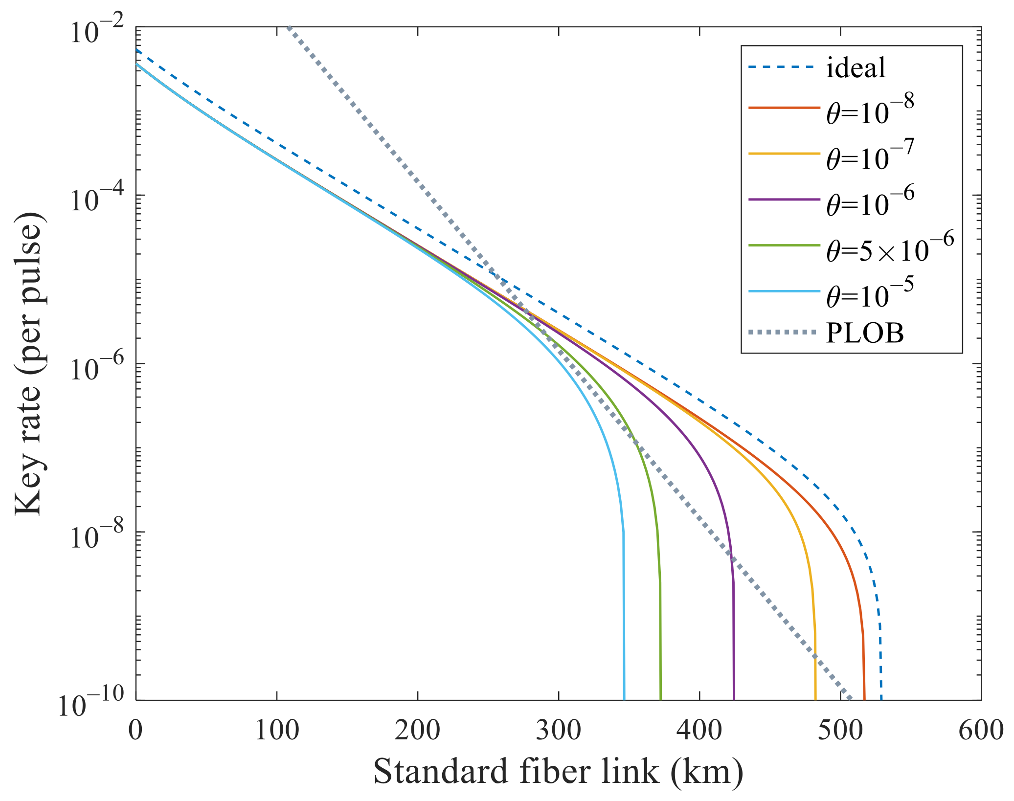
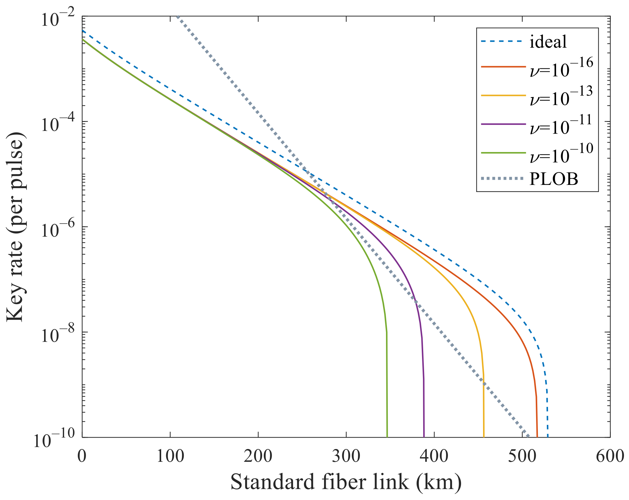
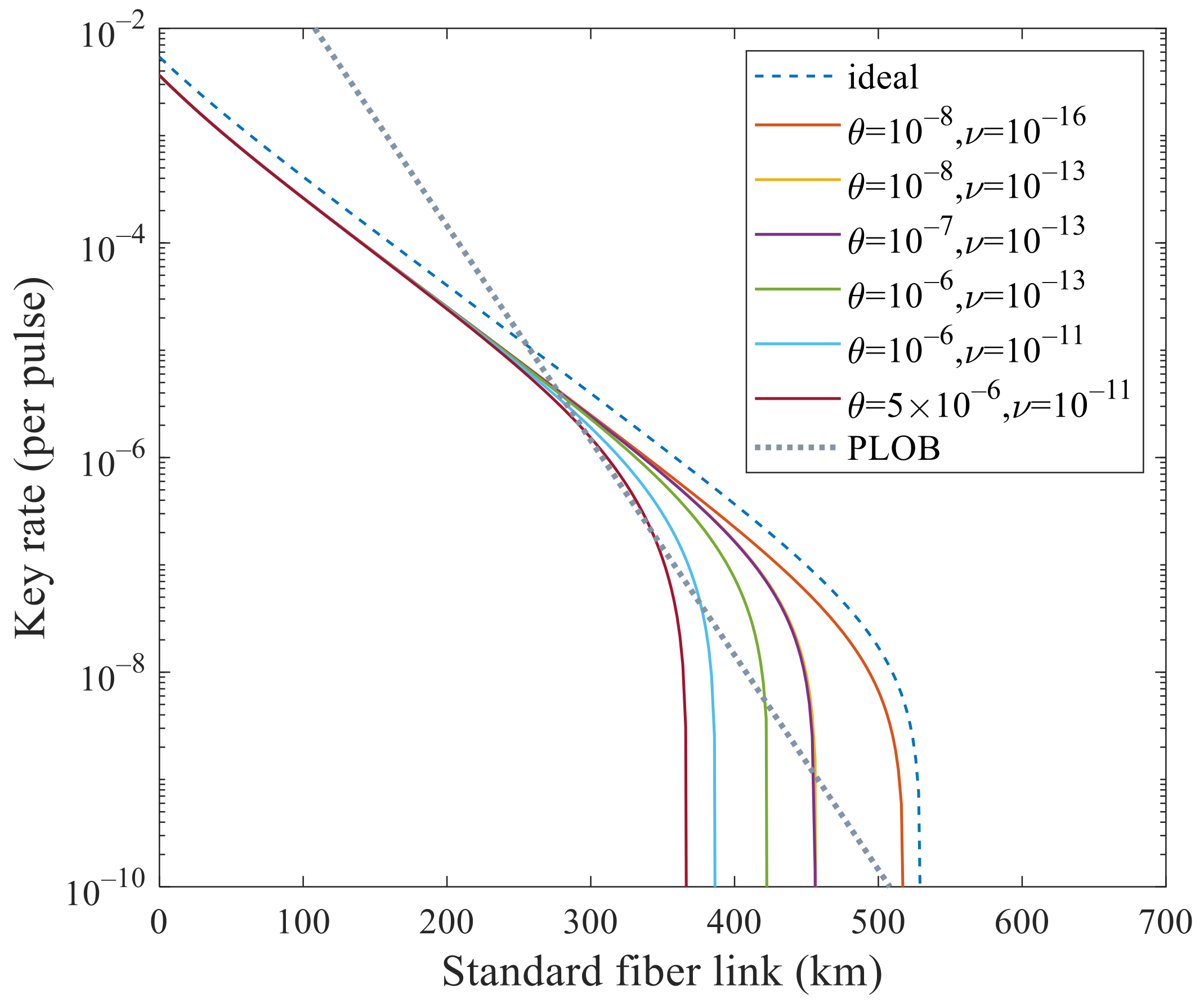
We mainly analyze its performance to surpass PLOB bound [9] under these experimental parameters with flawed and leaky sources. In Figure 1 and Figure 2, we analyze the effects of these two kinds of side channels separately. In Figure 1, the SKR can beat the PLOB bound when $\theta$ increases to $5\times {10}^{-6}$ but cannot when ${10}^{-5}$. In Figure 2, the SKR can beat the PLOB bound when $\nu$ increases to ${10}^{-11}$ but cannot when ${10}^{-10}$. Combining these two values, i.e., $\theta =5\times {10}^{-6}$ and $\nu ={10}^{-11}$, we can see that the SKR still can surpass the PLOB bound at 296 to 340 km in Figure 3. When $\theta ={10}^{-8}$ and $\nu ={10}^{-16}$, the SKR overlaps with that when $\theta =0$ and $\nu =0$, which means that the side channels will not affect the SKR at this time. We can see that the SKR is hardly affected by the side channels at a short distance, i.e., the lines overlap nearly before 200 km in Figure 1, Figure 2 and Figure 3. Also, we note that the SKR estimated with the method in this paper when without side channels is lower than that of [11,17,22] by comparing the dashed line with the solid line when $\theta =0$ and $\nu =0$ in Figure 3. Therefore, we could choose the original method [11,17,22] when without side channels and choose the method in this paper when with side channels.

6. Conclusions

In this paper, we take into account the imperfections at the light source and enhance the practical implementation of the SNS protocol. We analyze that the flaws of phase modulation can be overcome by regarding the deviation of the phase as phase noise and eliminating it with the method of the post-selection of phase. To overcome the side channels that may arise from THAs or device imperfections, we modify the GLT method [42] to the SNS protocol. Remarkably, we decompose the two-mode single-photon states into two special parts which are not the Pauli operators to reduce the number of parameters that need to be solved. To make it more practical, we analyze how to apply this method with the four-intensity decoy-state method. In this way, the practical implementations of the SNS protocol can be guaranteed without a detailed characterization of the side channels. Last, we note that the pulse correlations are not considered in this paper, which may be solved with the method in [28,33,34,36,50]. In conclusion, our results might constitute a crucial step towards guaranteeing the practical implementations of the SNS protocol with flawed and leaky sources.

References

1. Bennett, C.H.; Brassard, G. Quantum cryptography: Public key distribution and coin tossing. Theor. Comput. Sci. 2014, 560, 7–11. [Google Scholar] [CrossRef]
2. Pirandola, S.; Andersen, U.L.; Banchi, L.; Berta, M.; Bunandar, D.; Colbeck, R.; Englund, D.; Gehring, T.; Lupo, C.; Ottaviani, C.; et al. Advances in quantum cryptography. Adv. Opt. Photon. 2020, 12, 1012–1236. [Google Scholar] [CrossRef] [Green Version]
3. Xu, F.; Ma, X.; Zhang, Q.; Lo, H.K.; Pan, J.W. Secure quantum key distribution with realistic devices. Rev. Mod. Phys. 2020, 92, 025002. [Google Scholar] [CrossRef]
4. Hwang, W.Y. Quantum key distribution with high loss: Toward global secure communication. Phys. Rev. Lett. 2003, 91, 057901. [Google Scholar] [CrossRef] [Green Version]
5. Wang, X.B. Beating the photon-number-splitting attack in practical quantum cryptography. Phys. Rev. Lett. 2005, 94, 230503. [Google Scholar] [CrossRef] [PubMed] [Green Version]
6. Lo, H.K.; Ma, X.; Chen, K. Decoy state quantum key distribution. Phys. Rev. Lett. 2005, 94, 230504. [Google Scholar] [CrossRef] [Green Version]
7. Lo, H.K.; Curty, M.; Qi, B. Measurement-device-independent quantum key distribution. Phys. Rev. Lett. 2012, 108, 130503. [Google Scholar] [CrossRef] [Green Version]
8. Takeoka, M.; Guha, S.; Wilde, M.M. Fundamental rate-loss tradeoff for optical quantum key distribution. Nat. Commun. 2014, 5, 5235. [Google Scholar] [CrossRef]
9. Pirandola, S.; Laurenza, R.; Ottaviani, C.; Banchi, L. Fundamental limits of repeaterless quantum communications. Nat. Commun. 2017, 8, 15043. [Google Scholar] [CrossRef] [Green Version]
10. Lucamarini, M.; Yuan, Z.L.; Dynes, J.F.; Shields, A.J. Overcoming the rate-distance limit of quantum key distribution without quantum repeaters. Nature 2018, 557, 400–403. [Google Scholar] [CrossRef]
11. Wang, X.B.; Yu, Z.W.; Hu, X.L. Twin-field quantum key distribution with large misalignment error. Phys. Rev. A 2018, 98, 062323. [Google Scholar] [CrossRef] [Green Version]
12. Ma, X.; Zeng, P.; Zhou, H. Phase-Matching Quantum Key Distribution. Phys. Rev. X 2018, 8, 031043. [Google Scholar] [CrossRef] [Green Version]
13. Curty, M.; Azuma, K.; Lo, H.K. Simple security proof of twin-field type quantum key distribution protocol. NPJ Quant. Inf. 2019, 5, 64. [Google Scholar] [CrossRef]
14. Cui, C.; Yin, Z.Q.; Wang, R.; Chen, W.; Wang, S.; Guo, G.C.; Han, Z.F. Twin-Field Quantum Key Distribution without Phase Postselection. Phys. Rev. Appl. 2019, 11, 034053. [Google Scholar] [CrossRef] [Green Version]
15. Lin, J.; Lütkenhaus, N. Simple security analysis of phase-matching measurement-device-independent quantum key distribution. Phys. Rev. A 2018, 98, 042332. [Google Scholar] [CrossRef] [Green Version]
16. Tamaki, K.; Lo, H.; Wang, W.; Lucamarini, M. Information theoretic security of quantum key distribution overcoming the repeaterless secret key capacity bound. arXiv 2018, arXiv:1805.05511v1. [Google Scholar]
17. Yu, Z.W.; Hu, X.L.; Jiang, C.; Xu, H.; Wang, X.B. Sending-or-not-sending twin-field quantum key distribution in practice. Sci. Rep. 2019, 9, 3080. [Google Scholar] [CrossRef] [Green Version]
18. Jiang, C.; Yu, Z.W.; Hu, X.L.; Wang, X.B. Unconditional Security of Sending or Not Sending Twin-Field Quantum Key Distribution with Finite Pulses. Phys. Rev. Appl. 2019, 12, 024061. [Google Scholar] [CrossRef] [Green Version]
19. Wang, X.B.; Hu, X.L.; Yu, Z.W. Practical Long-Distance Side-Channel-Free Quantum Key Distribution. Phys. Rev. Appl. 2019, 12, 054034. [Google Scholar] [CrossRef] [Green Version]
20. Hu, X.L.; Jiang, C.; Yu, Z.W.; Wang, X.B. Sending-or-not-sending twin-field protocol for quantum key distribution with asymmetric source parameters. Phys. Rev. A 2019, 100, 062337. [Google Scholar] [CrossRef] [Green Version]
21. Zhou, X.Y.; Zhang, C.H.; Zhang, C.M.; Wang, Q. Asymmetric sending or not sending twin-field quantum key distribution in practice. Phys. Rev. A 2019, 99, 062316. [Google Scholar] [CrossRef] [Green Version]
22. Xu, H.; Yu, Z.W.; Jiang, C.; Hu, X.L.; Wang, X.B. Sending-or-not-sending twin-field quantum key distribution: Breaking the direct transmission key rate. Phys. Rev. A 2020, 101, 042330. [Google Scholar] [CrossRef]
23. Jiang, C.; Hu, X.L.; Xu, H.; Yu, Z.W.; Wang, X.B. Zigzag approach to higher key rate of sending-or-not-sending twin field quantum key distribution with finite-key effects. New J. Phys. 2020, 22, 053048. [Google Scholar] [CrossRef]
24. Lu, Y.F.; Wang, Y.; Jiang, M.S.; Liu, F.; Zhang, X.X.; Bao, W.S. Finite-key analysis of sending-or-not-sending twin-field quantum key distribution with intensity fluctuations. Quantum Inf. Process. 2021, 20, 135. [Google Scholar] [CrossRef]
25. Liu, Y.; Yu, Z.W.; Zhang, W.; Guan, J.Y.; Chen, J.P.; Zhang, C.; Hu, X.L.; Li, H.; Jiang, C.; Lin, J.; et al. Experimental Twin-Field Quantum Key Distribution through Sending or Not Sending. Phys. Rev. Lett. 2019, 123, 100505. [Google Scholar] [CrossRef] [Green Version]
26. Chen, J.P.; Zhang, C.; Liu, Y.; Jiang, C.; Zhang, W.; Hu, X.L.; Guan, J.Y.; Yu, Z.W.; Xu, H.; Lin, J.; et al. Sending-or-Not-Sending with Independent Lasers: Secure Twin-Field Quantum Key Distribution over 509 km. Phys. Rev. Lett. 2020, 124, 070501. [Google Scholar] [CrossRef] [Green Version]
27. Liu, H.; Jiang, C.; Zhu, H.T.; Zou, M.; Yu, Z.W.; Hu, X.L.; Xu, H.; Ma, S.; Han, Z.; Chen, J.P.; et al. Field Test of Twin-Field Quantum Key Distribution through Sending-or-Not-Sending over 428 km. Phys. Rev. Lett. 2021, 126, 250502. [Google Scholar] [CrossRef]
28. Pereira, M.; Kato, G.; Mizutani, A.; Curty, M.; Tamaki, K. Quantum key distribution with correlated sources. Sci. Adv. 2020, 6, 4487. [Google Scholar] [CrossRef]
29. Gottesman, D.; Lo, H.K.; Lütkenhaus, N.; Preskill, J. Security of quantum key distribution with imperfect devices. Quantum Inf. Comput. 2004, 4, 325–360. [Google Scholar]
30. Tamaki, K.; Curty, M.; Kato, G.; Lo, H.K.; Azuma, K. Loss-tolerant quantum cryptography with imperfect sources. Phys. Rev. A 2014, 90, 052314. [Google Scholar] [CrossRef] [Green Version]
31. Mizutani, A.; Curty, M.; Lim, C.C.W.; Imoto, N.; Tamaki, K. Finite-key security analysis of quantum key distribution with imperfect light sources. New J. Phys. 2015, 17, 093011. [Google Scholar] [CrossRef]
32. Tamaki, K.; Curty, M.; Lucamarini, M. Decoy-state quantum key distribution with a leaky source. New J. Phys. 2016, 18, 065008. [Google Scholar] [CrossRef]
33. Yoshino, K.I.; Fujiwara, M.; Nakata, K.; Sumiya, T.; Sasaki, T.; Takeoka, M.; Sasaki, M.; Tajima, A.; Koashi, M.; Tomita, A. Quantum key distribution with an efficient countermeasure against correlated intensity fluctuations in optical pulses. NPJ Quant. Inf. 2018, 4, 8. [Google Scholar] [CrossRef]
34. Mizutani, A.; Kato, G.; Azuma, K.; Curty, M.; Ikuta, R.; Yamamoto, T.; Imoto, N.; Lo, H.K.; Tamaki, K. Quantum key distribution with setting-choice-independently correlated light sources. NPJ Quant. Inf. 2019, 5, 8. [Google Scholar] [CrossRef] [Green Version]
35. Mizutani, A.; Sasaki, T.; Takeuchi, Y.; Tamaki, K.; Koashi, M. Quantum key distribution with simply characterized light sources. NPJ Quant. Inf. 2019, 5, 87. [Google Scholar] [CrossRef] [Green Version]
36. Wang, Y.; Primaatmaja, I.W.; Lavie, E.; Varvitsiotis, A.; Lim, C.C.W. Characterising the correlations of prepare-and-measure quantum networks. NPJ Quant. Inf. 2019, 5, 17. [Google Scholar] [CrossRef]
37. Navarrete, Á.; Pereira, M.; Curty, M.; Tamaki, K. Practical Quantum Key Distribution That is Secure Against Side Channels. Phys. Rev. Appl. 2021, 15, 034072. [Google Scholar] [CrossRef]
38. Sun, S.; Xu, F. Security of quantum key distribution with source and detection imperfections. New J. Phys. 2021, 23, 023011. [Google Scholar] [CrossRef]
39. Xu, F.; Wei, K.; Sajeed, S.; Kaiser, S.; Sun, S.; Tang, Z.; Qian, L.; Makarov, V.; Lo, H.K. Experimental quantum key distribution with source flaws. Phys. Rev. A 2015, 92, 032305. [Google Scholar] [CrossRef] [Green Version]
40. Tang, Z.; Wei, K.; Bedroya, O.; Qian, L.; Lo, H.K. Experimental measurement-device-independent quantum key distribution with imperfect sources. Phys. Rev. A 2016, 93, 042308. [Google Scholar] [CrossRef] [Green Version]
41. Boaron, A.; Boso, G.; Rusca, D.; Vulliez, C.; Autebert, C.; Caloz, M.; Perrenoud, M.; Gras, G.; Bussières, F.; Li, M.J.; et al. Secure Quantum Key Distribution over 421 km of Optical Fiber. Phys. Rev. Lett. 2018, 121, 190502. [Google Scholar] [CrossRef] [Green Version]
42. Pereira, M.; Curty, M.; Tamaki, K. Quantum key distribution with flawed and leaky sources. NPJ Quant. Inf. 2019, 5, 62. [Google Scholar] [CrossRef] [Green Version]
43. Tomamichel, M.; Lim, C.C.W.; Gisin, N.; Renner, R. Tight finite-key analysis for quantum cryptography. Nat. Commun. 2012, 3, 634. [Google Scholar] [CrossRef]
44. Sun, S.H.; Gao, M.; Jiang, M.S.; Li, C.Y.; Liang, L.M. Partially random phase attack to the practical two-way quantum-key-distribution system. Phys. Rev. A 2012, 85, 032304. [Google Scholar] [CrossRef] [Green Version]
45. Tang, Y.L.; Yin, H.L.; Ma, X.; Fung, C.H.F.; Liu, Y.; Yong, H.L.; Chen, T.Y.; Peng, C.Z.; Chen, Z.B.; Pan, J.W. Source attack of decoy-state quantum key distribution using phase information. Phys. Rev. A 2013, 88, 022308. [Google Scholar] [CrossRef] [Green Version]
46. Vakhitov, A.; Makarov, V.; Hjelme, D.R. Large pulse attack as a method of conventional optical eavesdropping in quantum cryptography. J. Mod. Opt. 2001, 48, 2023–2038. [Google Scholar] [CrossRef]
47. Jain, N.; Anisimova, E.; Khan, I.; Makarov, V.; Marquardt, C.; Leuchs, G. Trojan-horse attacks threaten the security of practical quantum cryptography. New J. Phys. 2014, 16, 123030. [Google Scholar] [CrossRef] [Green Version]
48. Lucamarini, M.; Choi, I.; Ward, M.B.; Dynes, J.F.; Yuan, Z.L.; Shields, A.J. Practical Security Bounds Against the Trojan-Horse Attack in Quantum Key Distribution. Phys. Rev. X 2015, 5, 031030. [Google Scholar] [CrossRef] [Green Version]
49. Huang, A.; Li, R.; Egorov, V.; Tchouragoulov, S.; Kumar, K.; Makarov, V. Laser-Damage Attack Against Optical Attenuators in Quantum Key Distribution. Phys. Rev. Appl. 2020, 13, 034017. [Google Scholar] [CrossRef] [Green Version]
50. Nagamatsu, Y.; Mizutani, A.; Ikuta, R.; Yamamoto, T.; Imoto, N.; Tamaki, K. Security of quantum key distribution with light sources that are not independently and identically distributed. Phys. Rev. A 2016, 93, 042325. [Google Scholar] [CrossRef] [Green Version]
51. Azuma, K. Weighted sums of certain dependent random variables. Tohoku Math. J. 1967, 19, 357–367. [Google Scholar] [CrossRef]
Figure 1. Secret key rate (per pulse) in logarithmic scale versus transmission distance between Alice and Bob when only one kind of side channel is considered. The dashed line corresponds to the ideal case without side channels that is estimated with the method in [11,17,22]. In addition, the dotted line is the PLOB bound. The solid lines correspond to the cases with different θ when ν = 0 estimated with the method in this paper. The lines correspond to θ = 0 and 10 8 are superimposed, which means that it will not affect SKR when θ is less than 10 8 . It can beat the PLOB bound when θ increases to 5 × 10 6 .
Entropy 23 01103 g001
Figure 2. Secret key rate (per pulse) in logarithmic scale versus transmission distance between Alice and Bob when only one kind of side channel is considered. The dashed line corresponds to the ideal case without side channels that is estimated with the method in [11,17,22]. In addition, the dotted line is the PLOB bound. The solid lines correspond to the cases with different ν when θ = 0 estimated with the method in this paper. The solid lines correspond to ν = 0 and 10 16 are superimposed, which means that it will not affect SKR when ν is less than 10 16 . It can surpass the PLOB bound when increasing ν to around 10 11 .
Entropy 23 01103 g002
Figure 3. Secret key rate (per pulse) in logarithmic scale versus transmission distance between Alice and Bob with both side channels θ and ν . The dashed line corresponds to the ideal case without side channels that is estimated with the method in [11,17,22]. In addition, the dotted line is the PLOB bound. The SKR when θ = 0 and ν = 0 overlaps with that when θ = 10 8 and ν = 10 16 . The SKR when θ = 10 8 , ν = 10 13 and θ = 10 7 , ν = 10 13 are superimposed. In addition, the SKR with θ = 10 6 and ν = 10 11 surpass the PLOB bound at 296 to 340 km.
Entropy 23 01103 g003