1. Introduction
Entropy-related concepts and information theory [
1,
2,
3,
4,
5,
6,
7,
8,
9] are useful for understanding complex dynamics in equilibrium and out of equilibrium. Examples include information (Shannon) entropy (measuring disorder, or lack of information) [
1], Fisher information [
2], relative entropy [
3], mutual information [
10], and their microscopic versions (e.g., trajectory entropy) [
11,
12], etc. In particular, while, in equilibrium, the Shannon entropy has a unique thermodynamic meaning, this is no longer the case in non-equilibrium, with different proposals for generalized entropies (e.g., see the review paper of Reference [
13] and references therein). Recent years have witnessed the increased awareness of information as a useful physical concept, for instance, in resolving the famous Maxwell’s demon paradox [
14], setting various thermodynamic inequality/uncertainty relations [
15,
16,
17], and establishing theoretical and conceptual links between physics and biology [
18]. Information-related ideas are also useful to uncover unexpected relations between apparently unrelated problems, for instance, the connections between Fisher information and Schrödinger equation, inspiring new development in non-equilibrium statistical mechanics [
19].
We have recently proposed information-geometric theory as a powerful tool to understand non-equilibrium stochastic processes that often involve high temporal variabilities and large fluctuations [
20,
21,
22,
23,
24,
25,
26,
27,
28,
29,
30,
31,
32], as often the case of rare, extreme events. This is based on the surprisal rate,
, where
is a probability density function (PDF) of a random variable
x at time
t, and
is a local entropy.
, informing how rapidly
or
changes in time, is especially useful for understanding time-varying non-equilibrium processes. As the name indicates, the surprisal rate
r measures the degree of surprise when
changes in time (no surprise in equilibrium with
). We can easily show that the average of the surprisal rate
since
. We note that, in this paper, averages refer to ensemble averages, which vary with time. A non-zero value is obtained from the second moment of
as
where
represents the information rate at which a new information is revealed (a new statistical state is accessed) due to time-evolution. Alternatively,
is the characteristic time scale over which information changes, linked to the smallest time scale of fluctuations [
17].
It is important to highlight that
,
, and
have the dimensions of (time)
, (time)
, and (time), respectively. In addition, we note that
is proportional to the average of an infinitesimal relative entropy (Kullback–Leibler divergence) (e.g., see Reference [
20]),
The total change in information between the initial time 0 and the time t is then obtained by integrating over time as which is the information length, quantifying the total number of statistically different states that a system passes through in time. In the limit of a Gaussian PDF where the variance is constant in time, one statistically distinguishable state is generated when a PDF peak moves by one standard deviation since the latter provides the uncertainty in measuring the peak position of the PDF. In a nutshell, is an information-geometric measure, enabling us to quantify how the “information” unfolds in time by dimensionless distance. Unlike other information measures, , , and are invariant under (time-independent) change of variables and are not system-specific. This non-system-specificity is especially useful for comparing the evolution of different variables/systems having different units.
Furthermore,
is a path-dependent dimensionless distance and is uniquely defined as a function of time for fixed parameters and initial condition. These properties are advantageous for quantifying correlation in time-varying data and understanding self-organization, long memory, and hysteresis involved in phase transitions [
20,
24,
27,
28,
29,
30,
32]. In particular, we recently investigated a non-autonomous Kramer equation by including a sudden perturbation to the system to mimic the onset of a sudden event [
32], demonstrating that our information rate predicts the onset of a sudden event better than one of the entropy-based measures (information flow) (see
Section 5.4 for details).
The purpose of this paper is to develop an information-geometric measure of causality (the causal information rate) by generalizing
(
). Like Reference [
32], our intention here is not on modeling the appearance of rare, extreme events (that are nonlinear, non-Gaussian) themselves, but on developing a new information-geometric causality method which is useful for predicting and understanding those events. The remainder of this paper is organized as follows. We propose the causal information rate in
Section 2 and apply it to the Kramers equation in
Section 3. One of the entropy-based methods (the information flow) is calculated in
Section 4 and is compared with our proposed method in
Section 5. Conclusions are provided in
Section 6.
Appendix A,
Appendix B and
Appendix C show some detailed steps involved in our calculations. We note that, while the usual convention in statistics and probability theory is to use upper case letters for random variables and lower case letters for their realizations, we do not make such distinctions in this paper as their meanings should be clear from the context.
2. Causal Information Rate
Information theoretical measures of causality are often based on entropy, joint entropy, conditional entropy, or mutual information, where the causality is measured by the improvement of the predictability of one of the variables at future time by the knowledge of the other variable, the improved predictability being measured by the decrease in entropy [
16,
33,
34,
35,
36,
37,
38,
39,
40,
41]. However, there have been questions raised as to whether predictability improvement (e.g., as measured by the Granger causality, transfer entropy) is directly linked to causality (e.g., Reference [
39]) and the suggestion that causality is better understood by performing an intervention experiment to measure the effect of the change (some type of perturbation or intervention) in one variable on another. In particular, spurious causalities between the two (observed) state variables can arise through unobserved state variables that interact with both (observed) state variables, calling for care in dealing with a system with more than two variables. On the other hand, to deal with strongly time-dependent data, the concepts of transfer entropy rate [
34], information flow [
16,
40,
41], etc., are proposed.
It is not the aim of this paper to provide detailed discussions about these methods, but to introduce a new information geometric measure of causality (see below) and to compare our new method with one of them (information flow) (see
Section 4). Our new information geometric measure of causality focuses on how one variable affects the information rate of another variable. To this end, we generalize
in Equation (
1) and define the causal information rate for multiple variables.
In order to demonstrate the basic idea required, it is instructive to consider a stochastic system consisting of two variables
and
which have a bivariate joint PDF
at different times
and
, its equal-time joint PDF
, and the conditional PDFs
, as well as marginal PDFs
and
. Using the index notation
, we then define causal information rate
for
from the variable
to
as follows:
Here,
for
was used.
represents the information rate of
with its characteristic timescale
. Note that the subscript
j in
denotes that the information rate is calculated for the variable
j. Since
contains the contribution from the variable
j itself and other variable
, we denote the (auto) contribution from
j-th itself (where the other variable
is frozen in time) by using the superscript *. That is,
represents the information rate of
for given (frozen)
. Subtracting
from
in Equation (
3) then gives us the contribution of dynamic (time-evolving)
to
, signifying how
instantaneously influences the information rate of
.
It is important to note that, as in the case of the information rate
or
, the calculation of
,
and
in Equations (
3)–(5) does not require the knowledge of the main governing equations (stochastic differential equations). This is because Equations (
3)–(5) can be calculated from any (numerical or experimental) data as long as time-dependent (marginal, joint) PDFs can be constructed. For instance, we used a time-sliding window method to construct time-dependent PDFs of different variables and then calculated
and
to analyze numerically generated time-series data for fusion turbulence [
26], time-series music data [
20], and numerically generated time-series data for global circulation model [
28]. However, it is not always clear how many hidden variables are in a given data set.
It is also useful to note that, as in the case of Equation (
2), Equation (5) can be shown to be related to the infinitesimal relative entropy as
The method presented above is for a stochastic process with two variables. For stochastic processes involving three or more variables (
,
), one way to proceed is to calculate multivariate PDFs, and then bivariate joint PDFs
and its equal-time joint PDF
, and marginal PDFs
and
, and then calculate the information rate from
to
, where
(
,
), via Equations (
3)–(5). This will give us an effective causal information rate. Another way is to deal with the multivariate PDFs directly (to be reported in future work).
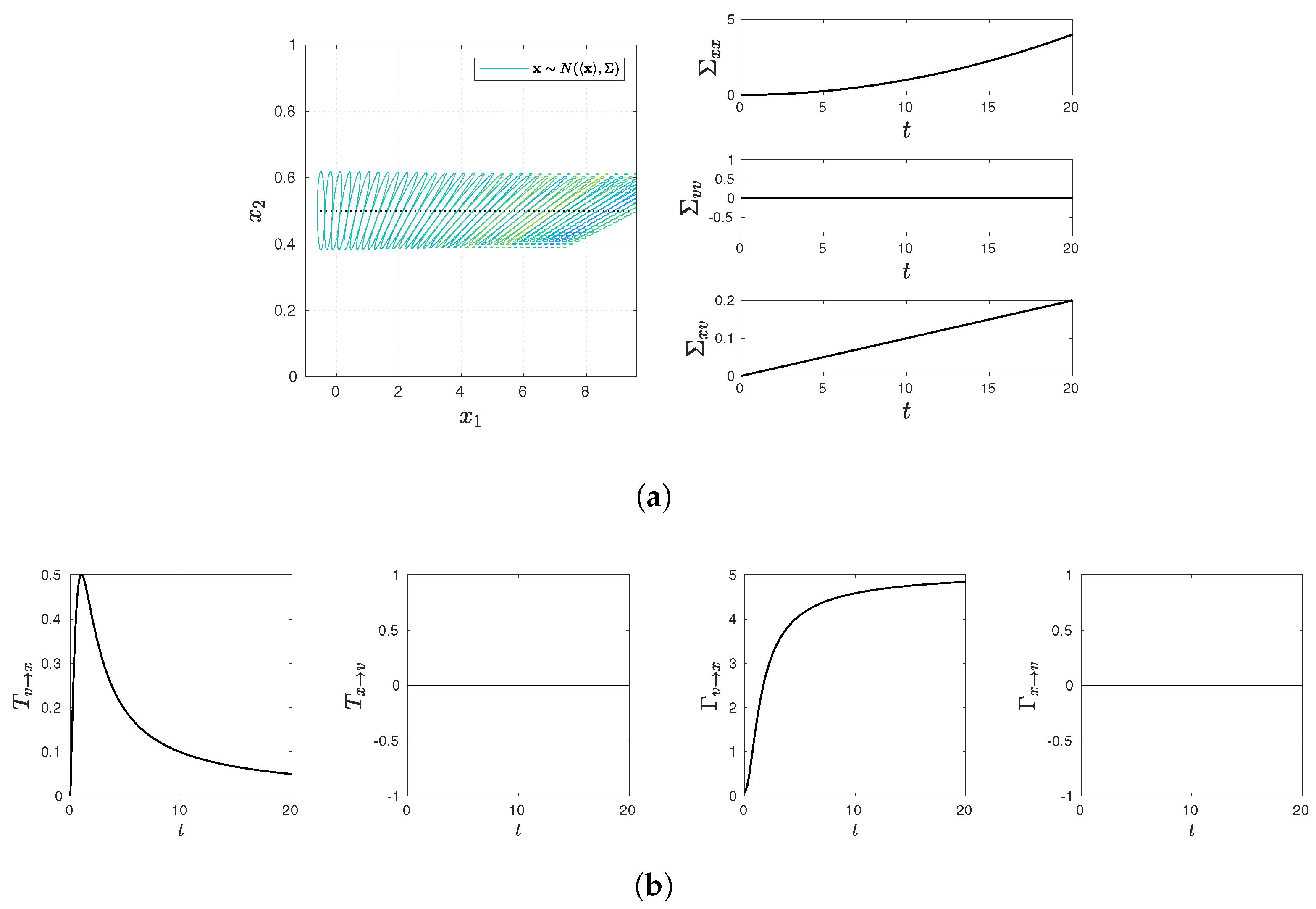
3. Kramers Equation
To demonstrate how the methods Equations (
3)–(5) work, in this section, we investigate an analytically solvable, Kramers equation, governed by the following Langevin equations [
31,
42]:
Here,
is a short (delta) correlated Gaussian noise with a zero average (mean)
and the strength
D with the following property:
where the angular brackets denote the average over
(
).
Assuming an initial Gaussian PDF, time-dependent PDFs remain Gaussian for all time. Thus, the bivariate joint PDF
and the marginal PDFs
and
are completely determined by covariance and mean values as
Here,
.
and
are the mean values.
is the covariance matrix with the elements
,
, and
, where
and
.
is the inverse of
, while
is the determinant.
Appendix A shows how to calculate mean values and the elements of covariance matrix.
Entropy of the joint PDF
and marginal PDFs
and
can easily be shown to be
On the other hand, the information rates for the equal-time joint PDF and the marginal PDFs are given by
It is useful to note that the first term on the RHS of Equations (17) and (18) is caused by the temporal change in the mean values of
x and
v, respectively, while the second term is due to that in the variance. Equation (
16) for the joint PDF contains the contribution from the temporal changes in the mean values of
x and
v and in the covariance matrix. The derivation of Equations (
16)–(18) is provided in
Appendix B (also see Reference [
31]).
To clarify the key idea behind the causality information rate, we provide detailed mathematical steps involved in the definition and calculation of
and
in
Section 3.1 and
Section 3.2, respectively.
3.1.
We start with the Kramers process Equations (
7)–(
9), where
is frozen for time
;
Then, the bivariate Gaussian PDF in Equation (
10) for a fixed
v takes the following form:
where
and
,
,
,
, and
.
For
and
in Equations (
3) and (5), we have
where
. In
Appendix B, we show that
is given by
Since
v is frozen during time
,
;
remains constant, while
and
change, as follows:
Then, to calculate the two terms on RHS of Equation (
25), we note
where
and
are given in Equations (27) and (28), while
is the inverse of the equal time covariance matrix. Using Equation (
29), we can show that the second term on RHS of Equation (
25) becomes
Here,
where
and
in Equations (27) and (28) are used. It is useful to note that
represents the rate at which the determinant of the covariance matrix changes in time for a fixed
v and becomes zero. This is because, for a fixed
v (essentially for
as seen below in regard to Equation (
52)), the evolution is conservative (reversible) where the phase space volume is conserved. Thus, the contribution from the variance to the information rate of
x for a given
v is solely determined by the temporal change in the cross-correlation
.
Finally, by using Equations (
30) and (
31) in Equation (
25), we have
It is interesting to compare the first term (caused by the mean motion
) on the RHS of Equation (
32) with that in Equation (17). For instance, if
,
, they take the same value. It should also be noted that, even when both
and
(as in equilibrium),
(unless
).
Putting Equations (17) and (
32) and
in Equation (
23) gives us
where we used
and
. (See
Appendix A for the values for means and covariance matrix.) Therefore, even when
, Equation (
33) can have a non-trivial contribution from a non-zero mean velocity.
To understand the difference between
and
, it is useful to define the following quantify
The cross-correlation
plays a more important role in Equation (
34) than in Equation (
33). For instance,
reduces Equation (
34) into a simple form
, with no contribution from the mean velocity
v. As noted above, such simplification does not occur for
in Equation (
33).
Nevertheless, if
and
, Equations (
33) and (
34) become
For instance, in equilibrium,
,
,
; thus,
. In
Section 3.2 below, we show that the equality
holds in equilibrium (see the discussion below Equation (
57)).
3.2.
We now consider the Kramers equation Equations (
7)–(
9), where
is frozen for time
;
Then, during
, the bivariate Gaussian PDF in Equation (
10) for a fixed
x takes the following form:
where
,
,
, and
.
We define
,
,
, and
as
where
is given in Equation (18). Note that Equation (43) simply follows by replacing
by
in Equation (
25).
Since we are considering the evolution of joint PDF of
v for a given
x for an infinitesimal time interval
through Equations (
36) and (37),
remains constant, while
and
evolve in time as follows:
Here, by using Equations (
7)–(
9), we can show (see
Appendix C for comments):
We now need to calculate the two terms on RHS of Equation (43). First, since
is frozen,
Secondly, using Equations (50) and (39), we can show that the second term on RHS of Equation (43) becomes
Here,
where we used Equations (
47) and (48). It is useful to note that
in Equation (
52), representing the rate at which the determinant of the covariance changes in time for a fixed
x, contains the two terms involving
(damping) and
D (stochasticity) due to irreversibility. We also note that, in equilibrium,
and
; thus,
;
, but
in Equation (
51), in general, contributing to
in Equation (43).
We use Equations (
49), (
51) and (
52) in Equation (43) to obtain
where
. Using Equation (
53) and (18) in Equation (
40) gives us
where
,
and
.
Again, to understand the difference between
and
, we perform straightforward but lengthy calculations using Equations (18), (41), (
52), and (
53) and find the following:
We again note that
plays a key role in Equation (
55), as in the case of Equation (
34). In particular, if
,
. If both
and
, Equations (
40) and (
55) become
In equilibrium where
and
,
and
. Thus, we have the equality
and
, as alluded to in the discussion following Equation (
35).
4. Entropy-Based Causality Measures
As noted previously, most of information theoretical measures of causality are based on entropy, joint entropy, conditional entropy, or mutual information, etc. Specifically, for the two dependent stochastic variables
and
with the marginal PDFs
and
and joint PDF
, entropy
, joint entropy
, mutual entropy
, and mutual information
are defined by
For Gaussian processes, Equations (
13)–(15) show that the entropy depends only on the variance/covariance, being independent of the mean value. This can be problematic as entropy fails to capture the effect of one variable on the mean value of another variable, for instance, caused by rare events associated with coherent structures, such as vortices, shear flows, etc. This is explicitly shown in
Section 5.4 (see Figure 5) in regard to causality. Although not widely recognized, it is important to point out the limitation of entropy-based measures in measuring perturbations (in particular, caused by abrupt events) that do not affect entropy, as shown in Reference [
32]. In addition, entropy has shortcomings, such as being non-invariant under coordinate transformations and insensitive to the local arrangement (shape) of
for fixed
t. Similar comments are applicable to other entropy-based measures. To demonstrate this point, in this section, we provide a detailed analysis of information flow based on conditional entropy [
16,
41].
4.1.
Information flow is based on predicting gain (or loss) of the future of subsystem 1 from the present state of subsystems 2 and defined as
where Equation (62) is used. Here, the first term and the second term on the RHS represent the rate of change of the marginal entropy of
and the rate of change of the conditional entropy of
conditional on
(i.e., frozen
v). The difference between these two rates then quantifies the effect of the evolution of
v on the entropy of
x. Note that
can be both negative and positive; a negative
means that
v acts to reduce the marginal entropy of
x (
), as numerically observed in Reference [
32].
Using Equation (
13), we have
. Then, by using Equations (
26)–(28) and (
29), we obtain
and
As can be seen from Equation (
65),
depends only on the variance, being independent of the mean value. Furthermore,
is proportional to the cross-correlation
, becoming zero for
as in the case of equilibrium. (Note that Equation (
65) is derived using a different method in Reference [
32] for the Kramers equation.)
4.2.
Similarly, information flow is based on predicting gain (or loss) of the future of subsystem 2 from the present state of subsystems 1 and defined as
where Equation (62) is used. Here, the first term and the second term on the RHS represent the rate of change of the marginal entropy of
and the rate of change of the conditional entropy of
conditional on
(i.e., frozen
x). The difference between these two rates then quantifies the effect of the evolution of
x on the entropy of
v. Note again that
can be both negative and positive; a negative
means that
x acts to reduce the marginal entropy of
v (
), as numerically observed in Reference [
32].
For
, we use Equations (
44)–(48) and (50) to obtain
Again, Equation (
68) is derived using a different method in Reference [
32]. As in the case of
in Equation (
65),
depends only on the variance, being independent of the mean value while being proportional to the cross-correlation
, becoming zero for
as in the case of equilibrium.
6. Conclusions
Information geometry in general concerns the distinguishability between two PDFs (e.g., constructed from data) and is sensitive to the local dynamics (e.g., Reference [
27]), depending on a local arrangement (the shape) of the PDFs. This is different from entropy, which is a global measure of a PDF, being insensitive to such a local arrangement. When a PDF is a continuous function of time, the information rate and information length are helpful in understanding far-from-equilibrium phenomena in terms of the number of distinguishable statistical states that a system evolves through in time. Being very sensitive to evolving dynamics, it enables us to compare different far-from-equilibrium processes using the same dimensionless distance, as well as quantifying the relation (correlation, self-regulation, etc.) among variables (e.g., References [
27,
28,
29,
30]).
In this paper, by extending our previous work [
20,
21,
22,
23,
24,
25,
26,
27,
28,
29,
30,
31], we introduced the causal information rate as a general information-geometric method that can elucidate causality relations in stochastic processes involving temporal variabilities and strong fluctuations. The key idea was to quantify the effect of one variable on the information rate of the other variable. The cross-correlation between the variables was shown to play a key role in the information flow, zero cross-correlation leading to zero information flow. In comparison, the causal information rate can take a non-zero value in the absence of cross-correlation. Since zero cross-correlation (measuring only the linear dependence) does not imply independence in general, this means that the causal information rate captures the (directional) dependence between two variables even when they are uncorrelated with each other.
Furthermore, the causal information rate captures the temporal change in both covariance matrix and mean value. In comparison, the information flow depends only on the temporal change in the covariance matrix. Thus, the causal information rate is a sensitive method for predicting an abrupt event and quantifying causal relations. These properties are welcome for predicting rare, large-amplitude events. Application has been made to the Kramers equation to highlight these points. Although the analysis in this paper is limited to the Gaussian variables that are entirely characterized by the mean and variance, similar results are likely to hold for non-Gaussian variables because the information rate captures the temporal changes of a PDF itself, while entropy-based measures (e.g., information flow) depend only on variance.
Given that causality (directional dependence) plays a crucial role in science and engineering (e.g., References [
43,
44]), our method could be useful in a wide range of problems. In particular, it could be utilized to elucidate causal relations among different players in nonlinear dynamical systems, fluid/plasma dynamics, laboratory plasmas, astrophysical systems, environmental science, finance, etc. For instance, in fluid/plasmas turbulence, it could help resolving the controversy over causality in the low-to-high (L-H) confinement transition [
29,
30,
45,
46], as well as contributing to identifying a causal relationship among different players responsible for the onset of sudden abrupt events (e.g., fusion plasmas eruption) (e.g., References [
47,
48]), with a better chance of control. It could also elucidate causal relationships among different physiological signals, how different parts of a human body (e.g., brain-heart-connection) are self-regulated to maintain homeostasis (the optimal living condition for survival), and how this homeostasis degrades with the onset of diseases.
Finally, it will be interesting to investigate the effects of coarse-graining in future works. In Reference [
49], for the information geometry given by the Fisher metric, relevant directions were shown to be exactly maintained under coarse-graining, while irrelevant directions contract. The analysis for more than two variables will also be addressed in future work.


