
A Non-Contact Fault Diagnosis Method for Bearings and Gears Based on Generalized Matrix Norm Sparse Filtering

Abstract
:1. Introduction
2. Proposed Method
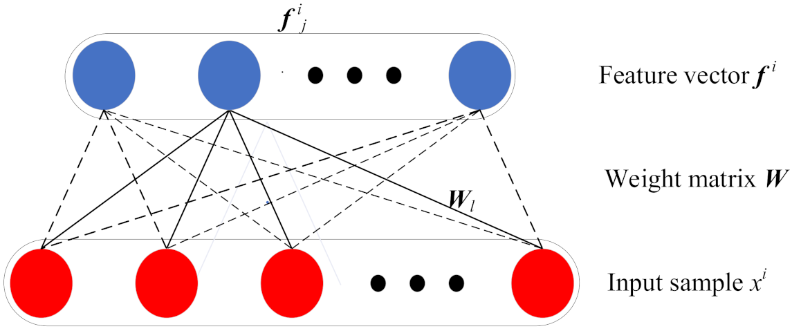
2.1. GMNSF
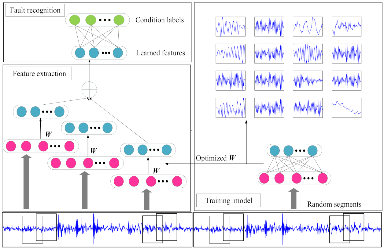
2.2. Intelligent Fault Diagnosis Framework
- Model training: The GMNSF model is trained through the original acoustic dataset. Set the training sample set as where is the number of samples, denotes the input variables in the sample, and is the label of the sample . The sample is randomly divided into segments and each segment includes input variables. Thus, a training set contains segments, where is the jth segment of the training dataset. Noticeably, the segments are obtained through overlapping. The following are the specific steps of model training. Then, the obtained is directly inputted to GMNSF to train the weight matrix W.
- Feature extraction: The discriminant features can be obtained by the optimal weight matrix . The training sample is separated into sections, and the is an integer and equal to . The dataset is composed of segments and . Then, the trained sparse filtering model is used to calculate the local feature of each sample. Learned features are obtained by combining local features using the average method, leading to
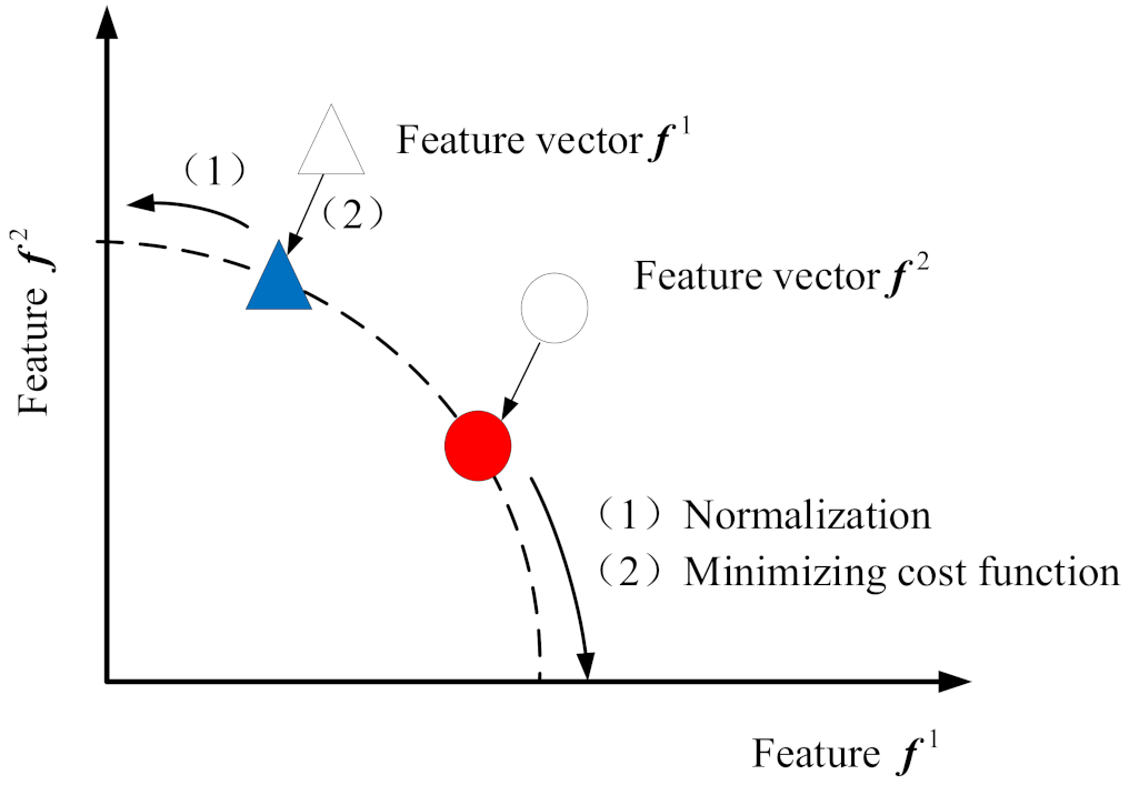
- Fault recognition: The learned features of all samples are combined with the labels and then trained through the softmax classifier. First, Z-Score is normalized to activate training and test data. The calculation method is as follows:where denotes the mean value of f, and represents the standard deviation. Thus, the rescaled matrix owns the properties of a standard normal distribution.Then, the softmax regression model is trained by the learned characteristic set and the healthy condition label set , . The softmax regression output probability that is the label of the feature vector. The softmax regression model of weight matrix is acquired by minimizing the nest cost function.where 1{.} is the indicator function, M denotes the training sample size, and D denotes the category number. λ is the parameter of the weight decay term.
3. Experimental Validation
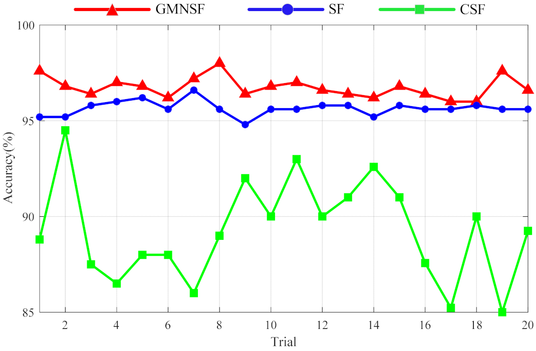
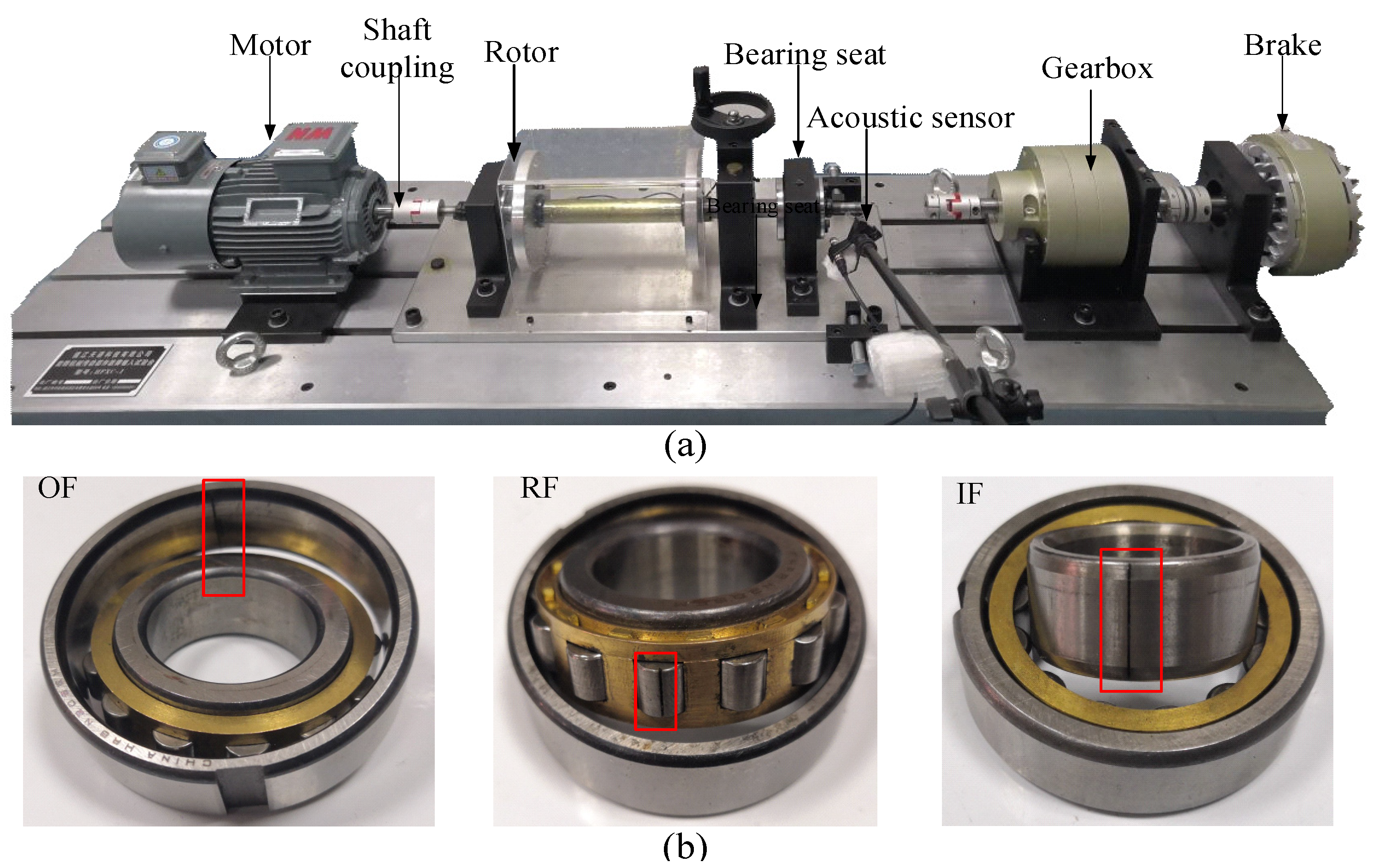
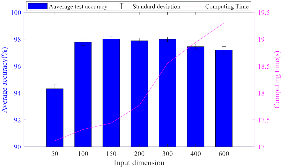
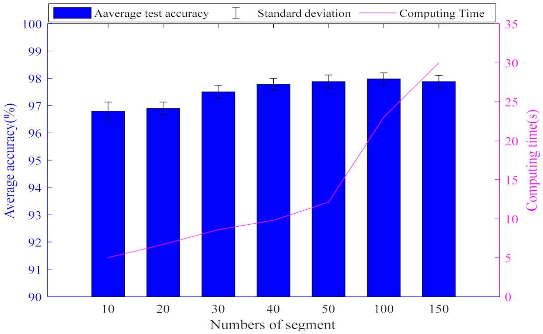
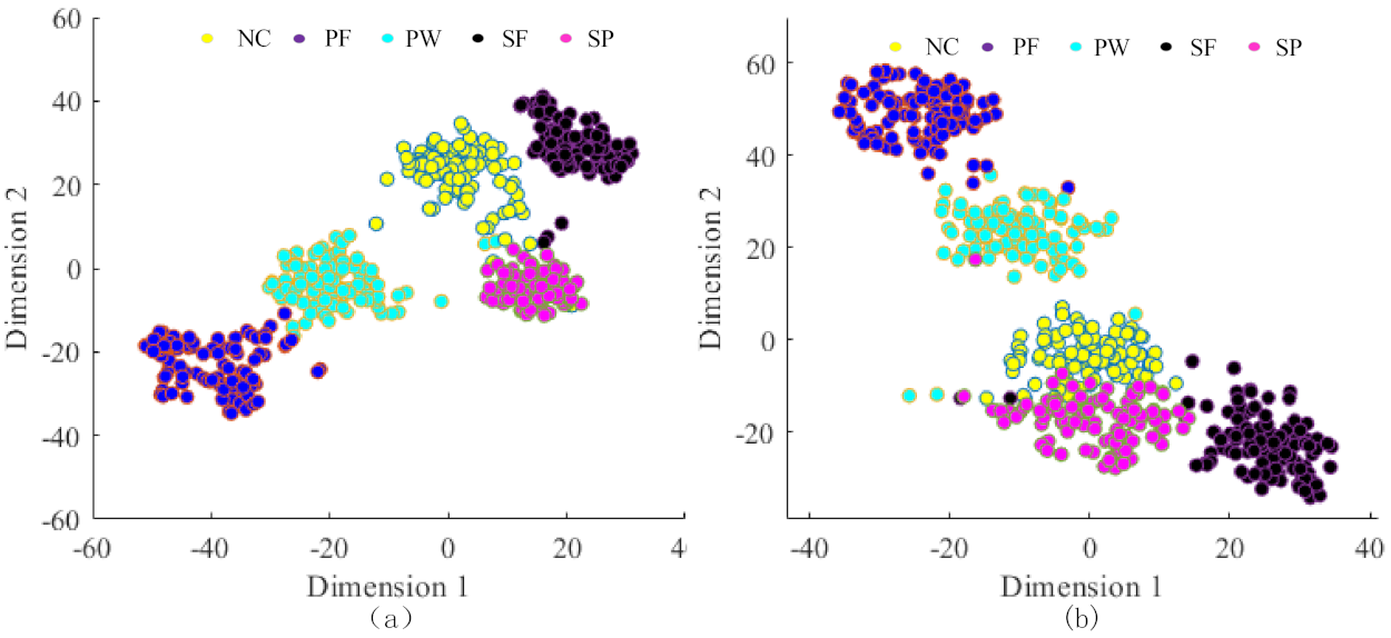
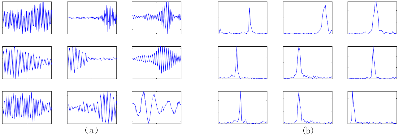
3.1. Rolling Bearing Data Verification and Analysis
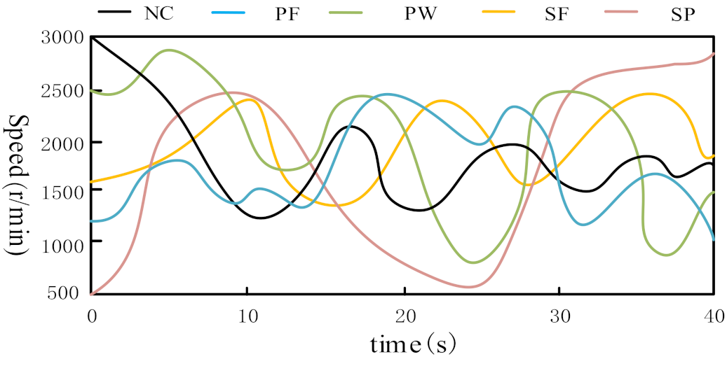
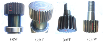
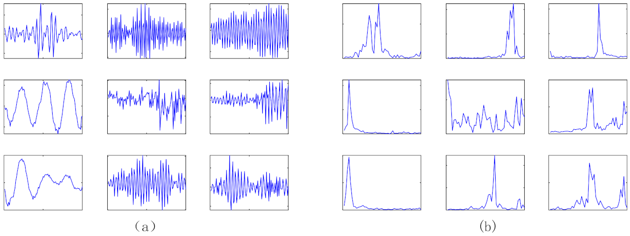
3.2. Gear Data Verification and Analysis
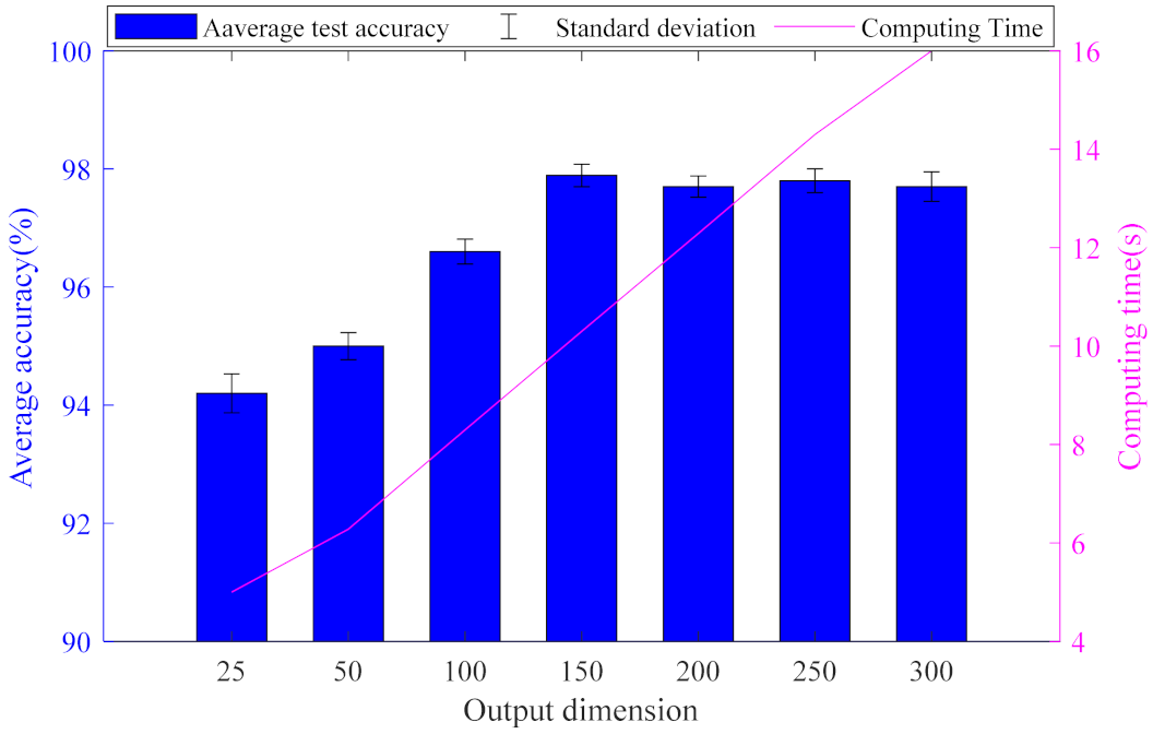
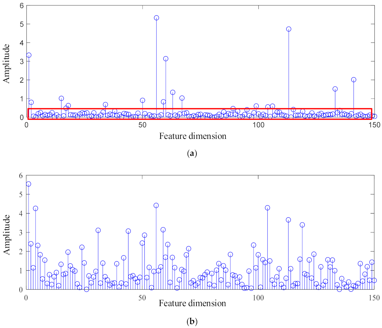
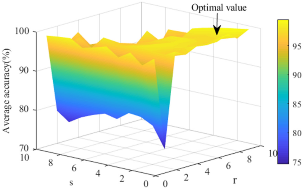
4. Discuss Weight Matrix
5. Conclusions
Author Contributions
Funding
Institutional Review Board Statement
Informed Consent Statement
Data Availability Statement
Acknowledgments
Conflicts of Interest
References
- Cheng, C.; Wang, J.; Chen, H. A Review of Intelligent Fault Diagnosis for High-Speed Trains: Qualitative Approaches. Entropy 2021, 23, 1. [Google Scholar] [CrossRef] [PubMed]
- Chen, H.; Jiang, B.; Ding, S. Data-driven fault diagnosis for traction systems in high-speed trains: A survey, challenges, and perspectives. IEEE Trans. Intell. Transp. Syst. 2020, 1–17. [Google Scholar] [CrossRef]
- Jia, F.; Lei, Y.G.; Lin, J.; Zhou, X.; Lu, N. Deep neural networks: A promising tool for fault characteristic mining and intelligent diagnosis of rotating machinery with massive data. Mech. Syst. Signal Process. 2016, 73, 303–315. [Google Scholar] [CrossRef]
- Saufi, S.R.; Ahmad, Z.; Leong, M.S. Challenges and Opportunities of Deep Learning Models for Machinery Fault Detection and Diagnosis. A Review IEEE Access 2019, 7, 122644–122662. [Google Scholar] [CrossRef]
- Wang, J.R.; Li, S.M.; An, Z.H.; Jiang, X.; Qian, W.; Ji, S. Batch-normalized deep neural networks for achieving fast intelligent fault diagnosis of machines. Neurocomputing 2019, 329, 53–65. [Google Scholar] [CrossRef]
- Li, G.; Deng, C.; Wu, J. Sensor data-driven bearing fault diagnosis based on deep convolutional neural networks and S-transform. Sensors 2019, 19, 2750. [Google Scholar] [CrossRef] [PubMed] [Green Version]
- Yu, K.; Lin, T.R.; Ma, H.; Li, X. A multi-stage semi-supervised learning approach for intelligent fault diagnosis of rolling bearing using data augmentation and metric learning. Mech. Syst. Signal Process. 2018, 46, 107043. [Google Scholar] [CrossRef]
- Xin, B.; Wang, T.; Zheng, Y.; Wang, Y. A sparse autoencoder and softmax regression based diagnosis method for the attachment on the blades of marine current turbine. Sensors 2019, 19, 826. [Google Scholar]
- Jia, F.; Lei, Y.G.; Guo, L.; Lin, J.; Xing, S. A neural network constructed by deep learning technique and its application to intelligent fault diagnosis of machines. Neurocomputing 2018, 272, 619–628. [Google Scholar] [CrossRef]
- O’Brien, R.; Fontana, J.; Ponso, N. A pattern recognition system based on acoustic signals for fault detection on composite materials. Eur. J. Mech. A Solids 2017, 64, 1–10. [Google Scholar] [CrossRef]
- Han, B.; Zhang, X.; Wang, J. Hybrid distance-guided adversarial network for intelligent fault diagnosis under different working conditions. Measurement 2021, 176, 109197. [Google Scholar] [CrossRef]
- Wang, J.; Ji, S.; Han, B. Intelligent fault diagnosis for rotating machinery using L1/2-SF under variable rotational speed. Proc. Inst. Mech. Eng. Part D J. Automob. Eng. 2021, 235, 1409–1422. [Google Scholar] [CrossRef]
- Han, B.; Ji, S.; Wang, J. An intelligent diagnosis framework for roller bearing fault under speed fluctuation condition. Neurocomputing 2021, 420, 171–180. [Google Scholar] [CrossRef]
- Wang, Y.S.; Ren, X.M.; Yang, Y.F.; Deng, W.Q. Fault Signal Denoising Source Analysis of Rotating Machinery. Noise Vib. Control 2013, 33, 181–186. [Google Scholar]
- Zhang, H.; Lu, S.; He, Q. Multi-bearing defect detection with trackside acoustic signal based on a pseudo time–frequency analysis and Dopplerlet filter. Mech. Syst. Signal Process. 2016, 70–71, 176–200. [Google Scholar] [CrossRef]
- Zhang, D.; Stewart, E.; Entezami, M. Intelligent acoustic-based fault diagnosis of roller bearings using a deep graph convolutional network. Measurement 2020, 156, 107585. [Google Scholar] [CrossRef]
- Liu, H.; Li, L.; Ma, J. Rolling Bearing Fault Diagnosis Based on STFT-Deep Learning and Sound Signals. Shock Vib. 2016, 6, 6127479.1–6127479.12. [Google Scholar] [CrossRef] [Green Version]
- Glowacz, A. Acoustic based fault diagnosis of three-phase induction motor. Appl. Acoust. 2018, 137, 82–89. [Google Scholar] [CrossRef]
- Parvathi, S.; Hemamalini, S. Rational-dilation wavelet transform based torque estimation from acoustic signals for fault diagnosis in a three-phase induction motor. IEEE Trans. Ind. Inform. 2019, 115, 3492–3501. [Google Scholar]
- Cheng, H.; Liu, Z.; Yang, L.; Chen, X. Sparse representation and learning in visual recognition: Theory and applications. Signal Process 2013, 93, 1408–1425. [Google Scholar] [CrossRef]
- Wen, L.; Gao, L.; Li, X. A new deep transfer learning based on sparse auto-encoder for fault diagnosis. IEEE Trans. Syst. Man Cybern. Syst. 2017, 49, 136–144. [Google Scholar] [CrossRef]
- Lee, H.; Ekanadham, C.; Ng, A.Y. Sparse deep belief net model for visual area V2. In Proceedings of the Advances in Neural Information Processing Systems 21: 22nd Annual Conference on Neural Information Processing Systems, Vancouver, BC, Canada, 8–10 December 2008; pp. 873–880. [Google Scholar]
- Lee, H.; Battle, A.; Raina, R.; Ng, A.Y. Efficient sparse coding algorithms. In Proceedings of the Advances in Neural Information Processing Systems 20: 21st Annual Conference on Neural Information Processing Systems, Vancouver, BC, Canada, 3–6 December 2007; pp. 801–808. [Google Scholar]
- Ngiam, J.; Chen, Z.; Bhaskar, S.A.; Koh, P.W.; Ng, A.Y. Sparse filtering. In Proceedings of the 24th International Conference Neural Information Processing Systems, Granada, Spain, 12–15 December 2011; pp. 1125–1133. [Google Scholar]
- Wei, L.; Qiu, M.; Zhu, Z. Fault diagnosis of rolling element bearings with a spectrum searching method. Meas. Sci. Technol. 2017, 28, 095008. [Google Scholar]
- Zhang, Z.; Li, S.; Wang, J.; Xin, Y.; An, Z. General normalized sparse filtering: A novel unsupervised learning method for rotating machinery fault diagnosis MechSyst. Signal Process 2019, 124, 596–612. [Google Scholar] [CrossRef]
- Lei, Y.; Jia, F.; Lin, J.; Xing, S.; Ding, S.X. An Intelligent Fault Diagnosis Method Using Unsupervised Feature Learning towards Mechanical Big Data. IEEE Trans. Ind. Electron. 2016, 63, 3137–3147. [Google Scholar] [CrossRef]
- Zhang, Z.; Li, S.; Lu, J. A novel intelligent fault diagnosis method based on fast intrinsic component filtering and pseudo-normalization. Mech. Syst. Signal Process. 2020, 145, 106923. [Google Scholar] [CrossRef]
- Jia, X.; Zhao, M.; Di, Y. Investigation on the kurtosis filter and the derivation of convolutional sparse filter for impulsive signature enhancement. J. Sound Vib. 2017, 386, 433–448. [Google Scholar] [CrossRef]
- Pezzotti, N.; Lelieveldt, B.P.; Van Der Maaten, L.; Höllt, T.; Eisemann, E.; Vilanova, A. Approximated and User Steerable tSNE for Progressive Visual Analytics. IEEE Trans. Vis. Comput. Graph. 2017, 23, 1739–1752. [Google Scholar] [CrossRef] [Green Version]
- Masson, G.S.; Busettini, C.; Miles, F.A. Vergence eye movements in response to binocular disparity without depth perception. Nature 1997, 389, 283–289. [Google Scholar] [CrossRef]


| Method | Description | Training Samples (%) | Testing Accuracy (%) |
|---|---|---|---|
| 1 | SF | 50 | 92.96 ± 1.22% |
| 2 | ICF | 50 | 87.35 ± 1.58% |
| 4 | CSF | 50 | 73.35 ± 3.78% |
| 5 | GMNSF | 50 | 97.93 ± 0.96% |
Publisher’s Note: MDPI stays neutral with regard to jurisdictional claims in published maps and institutional affiliations. |
© 2021 by the authors. Licensee MDPI, Basel, Switzerland. This article is an open access article distributed under the terms and conditions of the Creative Commons Attribution (CC BY) license (https://creativecommons.org/licenses/by/4.0/).
Share and Cite
Bao, H.; Shi, Z.; Wang, J.; Zhang, Z.; Zhang, G. A Non-Contact Fault Diagnosis Method for Bearings and Gears Based on Generalized Matrix Norm Sparse Filtering. Entropy 2021, 23, 1075. https://doi.org/10.3390/e23081075
Bao H, Shi Z, Wang J, Zhang Z, Zhang G. A Non-Contact Fault Diagnosis Method for Bearings and Gears Based on Generalized Matrix Norm Sparse Filtering. Entropy. 2021; 23(8):1075. https://doi.org/10.3390/e23081075
Chicago/Turabian StyleBao, Huaiqian, Zhaoting Shi, Jinrui Wang, Zongzhen Zhang, and Guowei Zhang. 2021. "A Non-Contact Fault Diagnosis Method for Bearings and Gears Based on Generalized Matrix Norm Sparse Filtering" Entropy 23, no. 8: 1075. https://doi.org/10.3390/e23081075
APA StyleBao, H., Shi, Z., Wang, J., Zhang, Z., & Zhang, G. (2021). A Non-Contact Fault Diagnosis Method for Bearings and Gears Based on Generalized Matrix Norm Sparse Filtering. Entropy, 23(8), 1075. https://doi.org/10.3390/e23081075