
Numerical Simulation of Swirl Flow Characteristics of CO2 Hydrate Slurry by Short Twisted Band


Abstract
:1. Introduction
2. Numerical Simulation Method
2.1. Physical Model
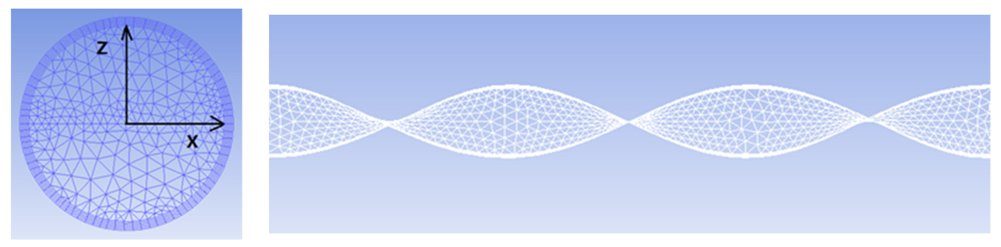
2.1.1. Geometric Model
2.1.2. Boundary Conditions
2.2. Meshing
2.3. Mathematical Model
2.3.1. Governing Equations
2.3.2. Discrete Phase Model
2.4. Calculation Method
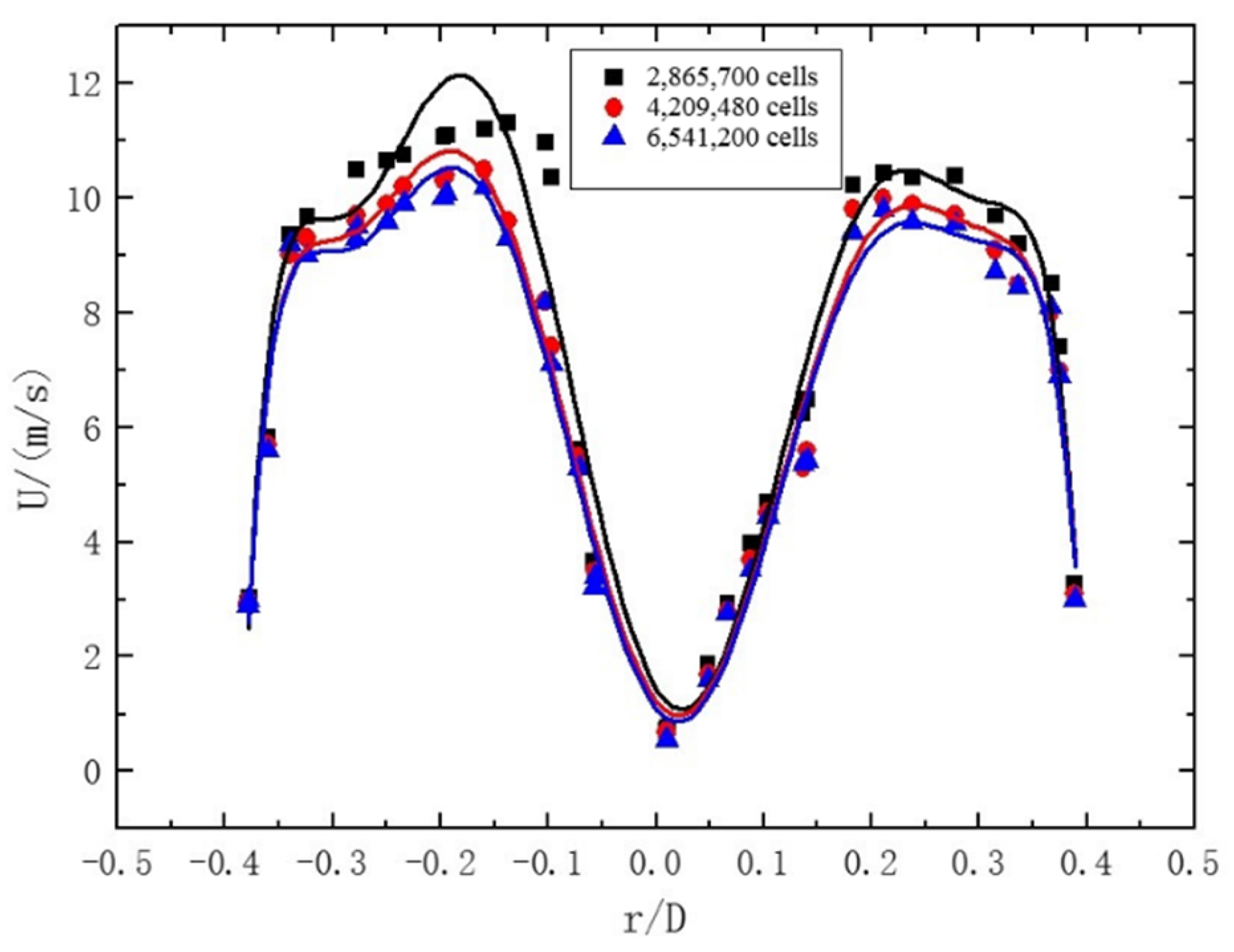
2.5. Grid Independence Test
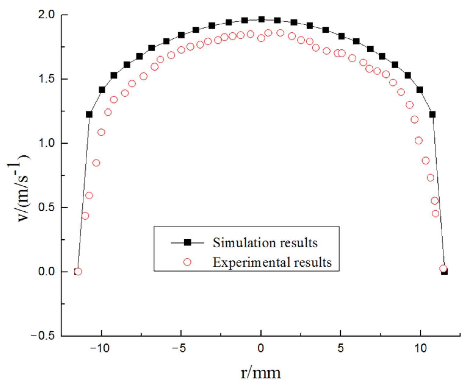
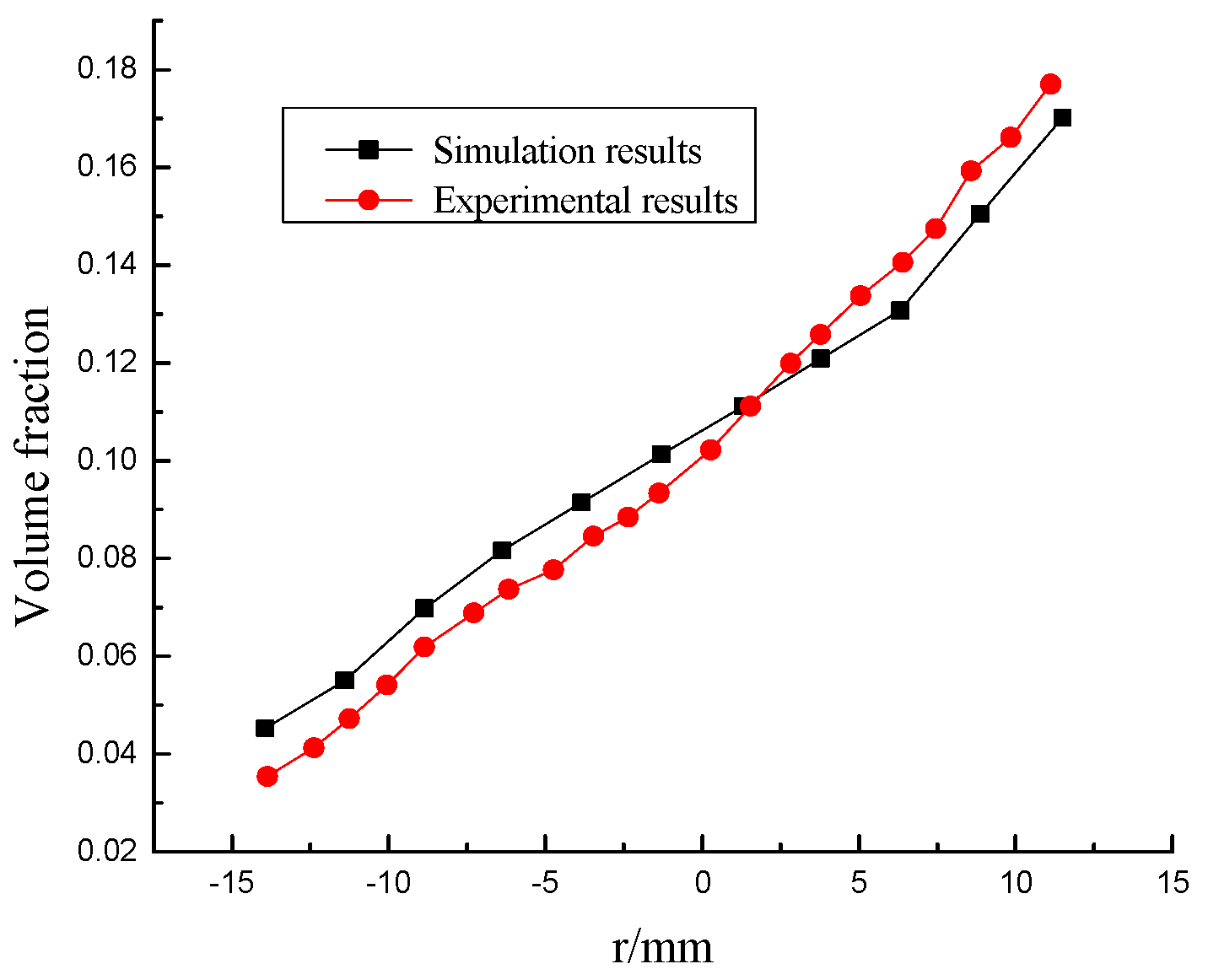
2.6. Experimental Verification
3. Results and Discussion
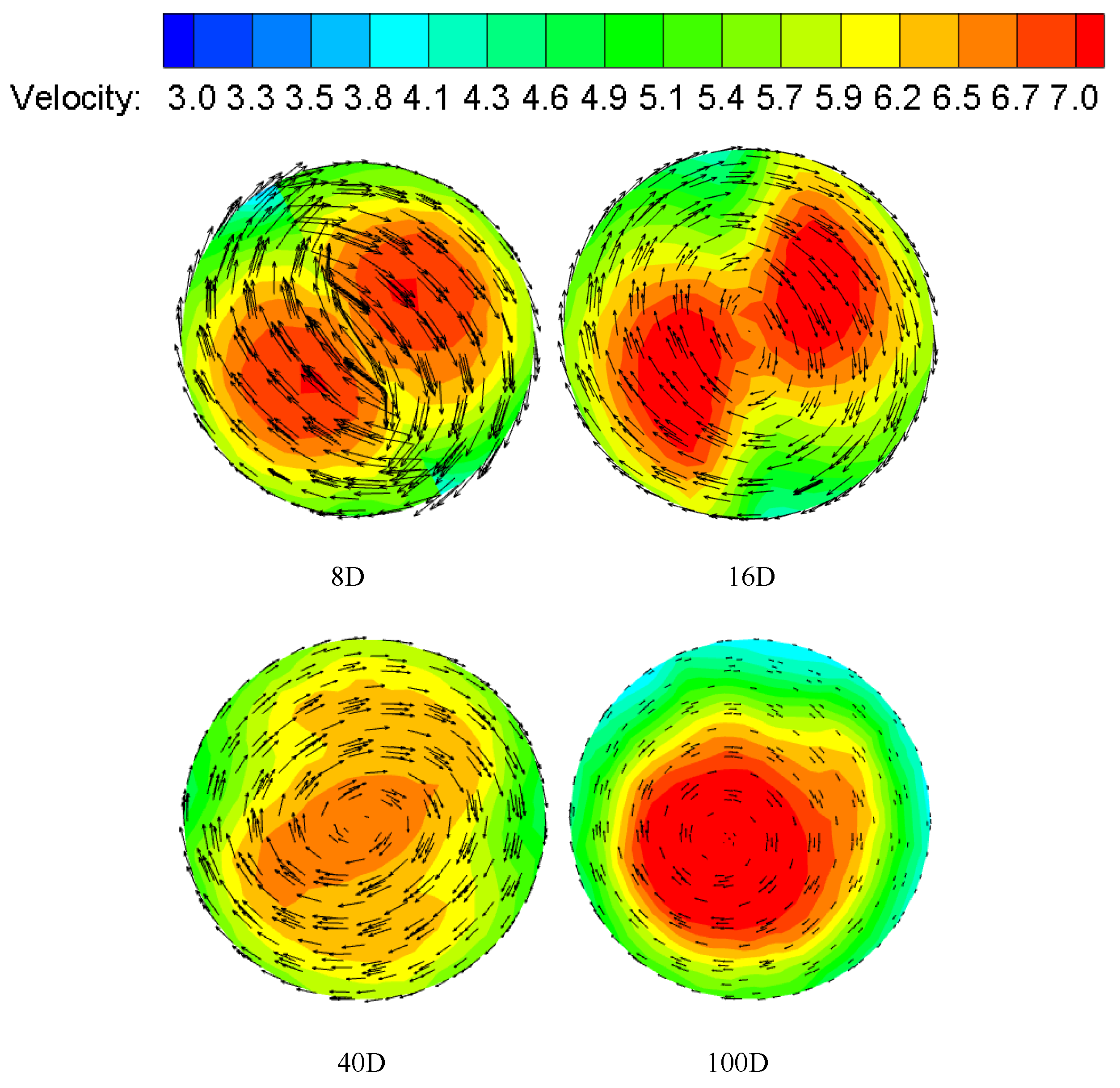
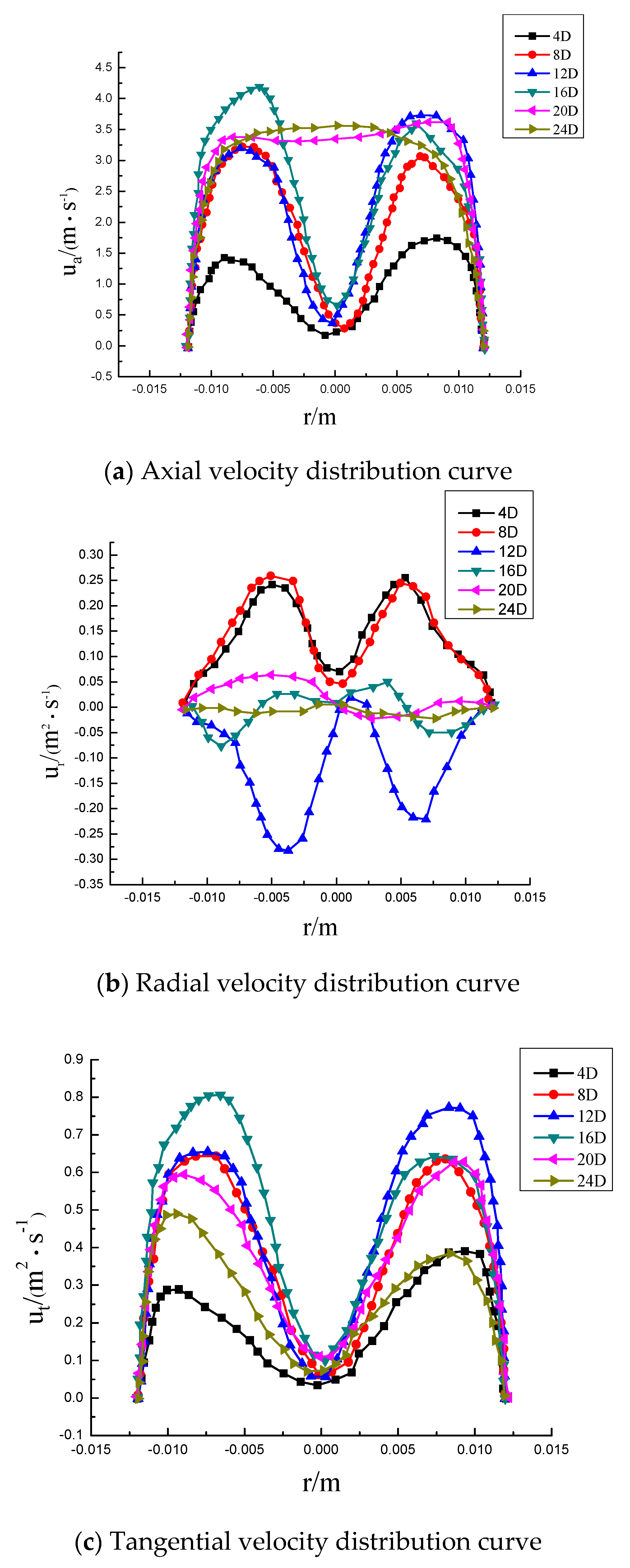
3.1. Velocity Distribution
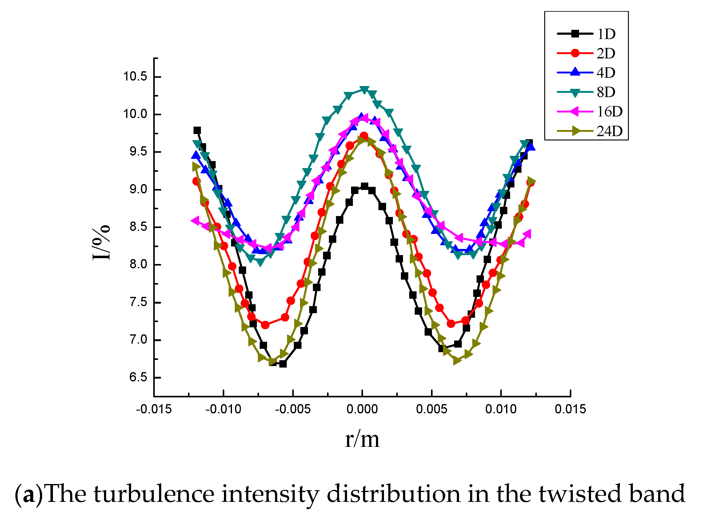
3.2. Turbulence Intensity
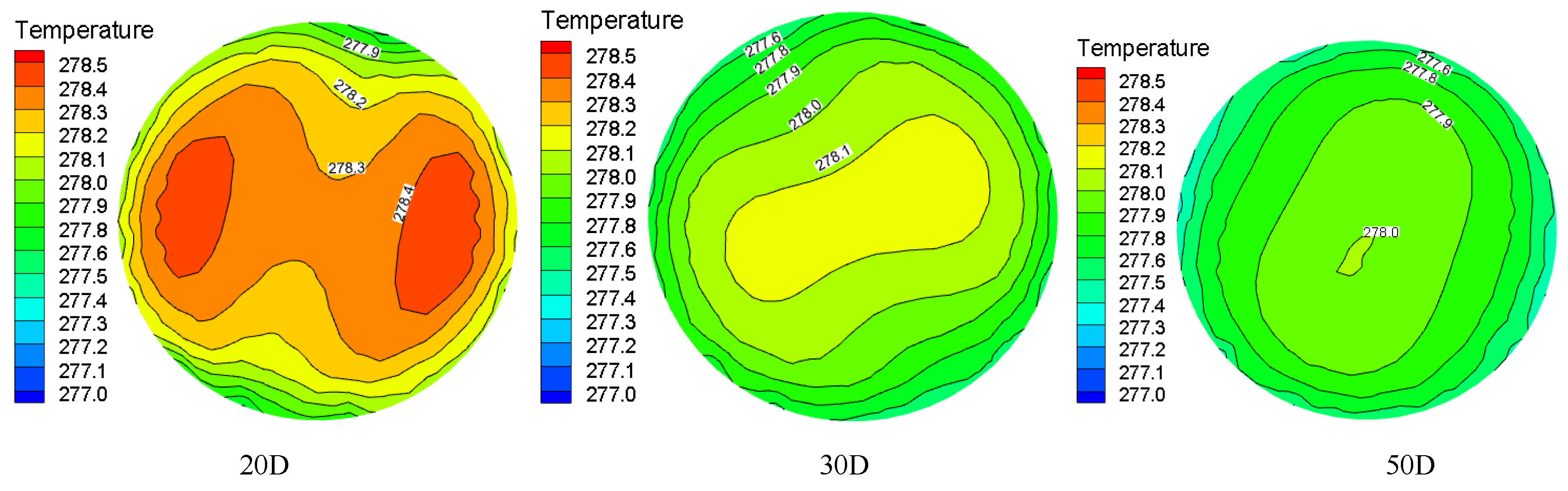
3.3. Temperature Distribution
3.4. Vortex Line Distribution
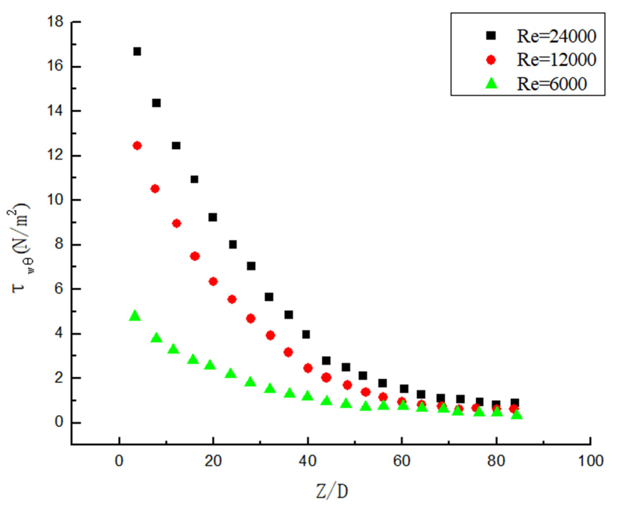
3.5. Attenuation Law of Wall Shear Stress
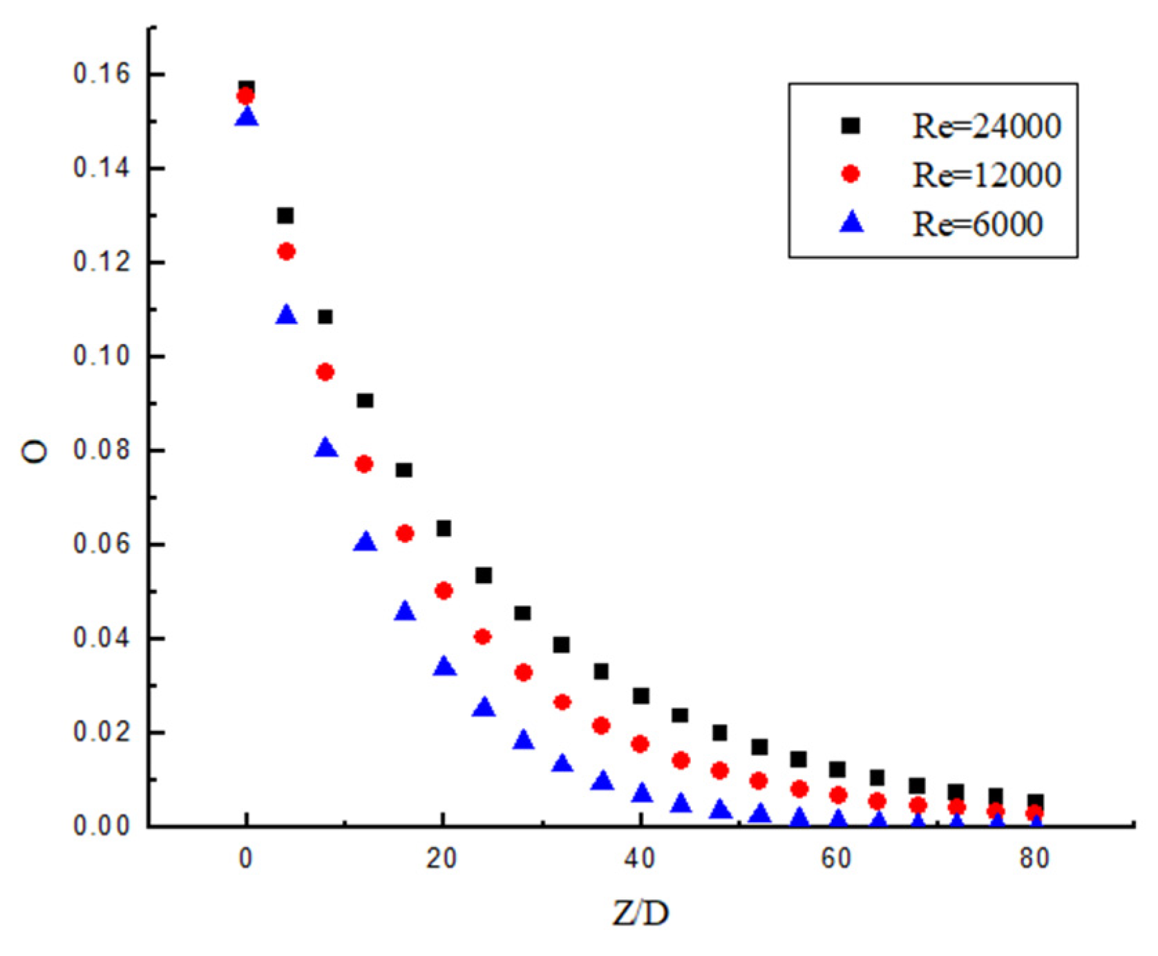
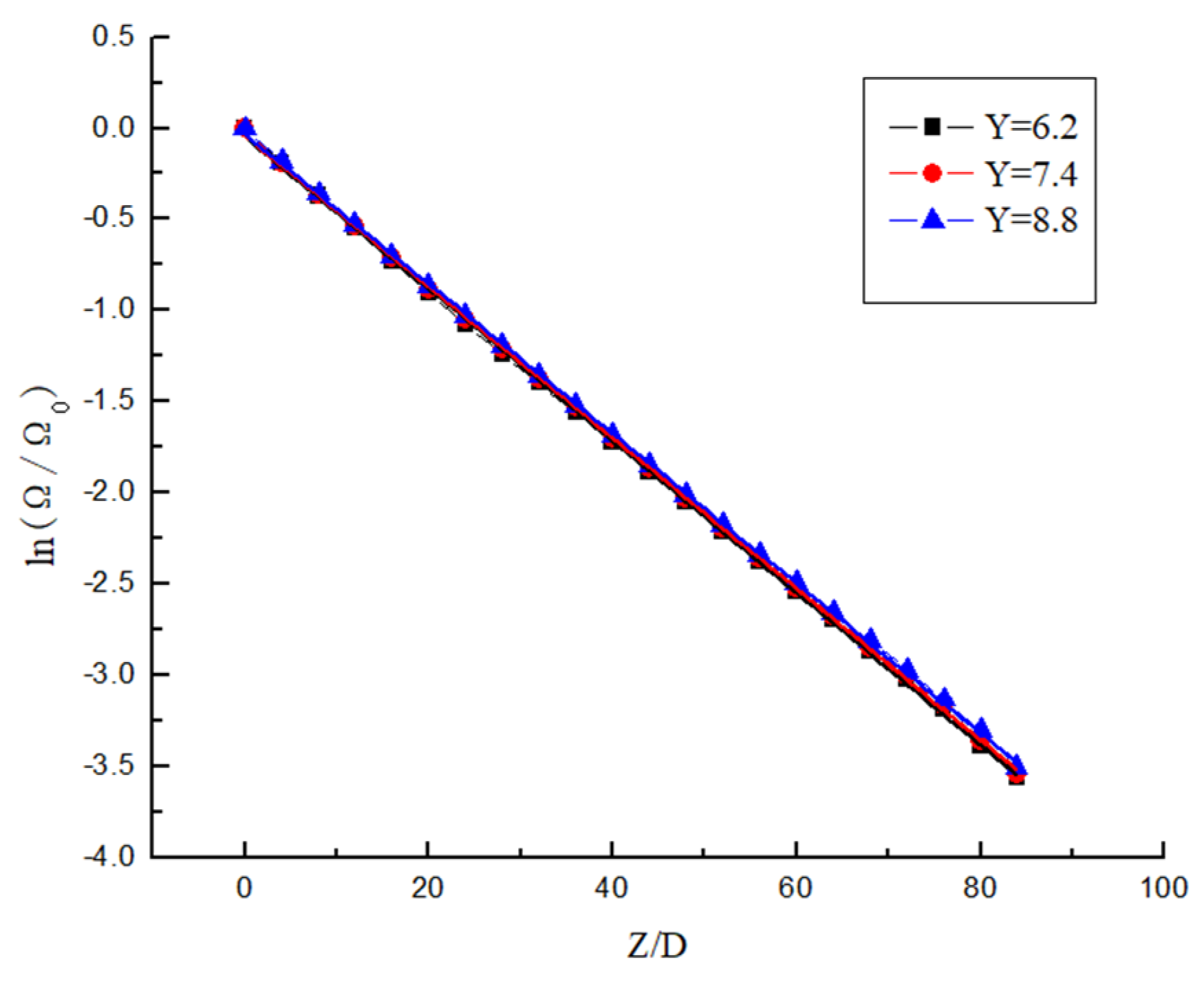
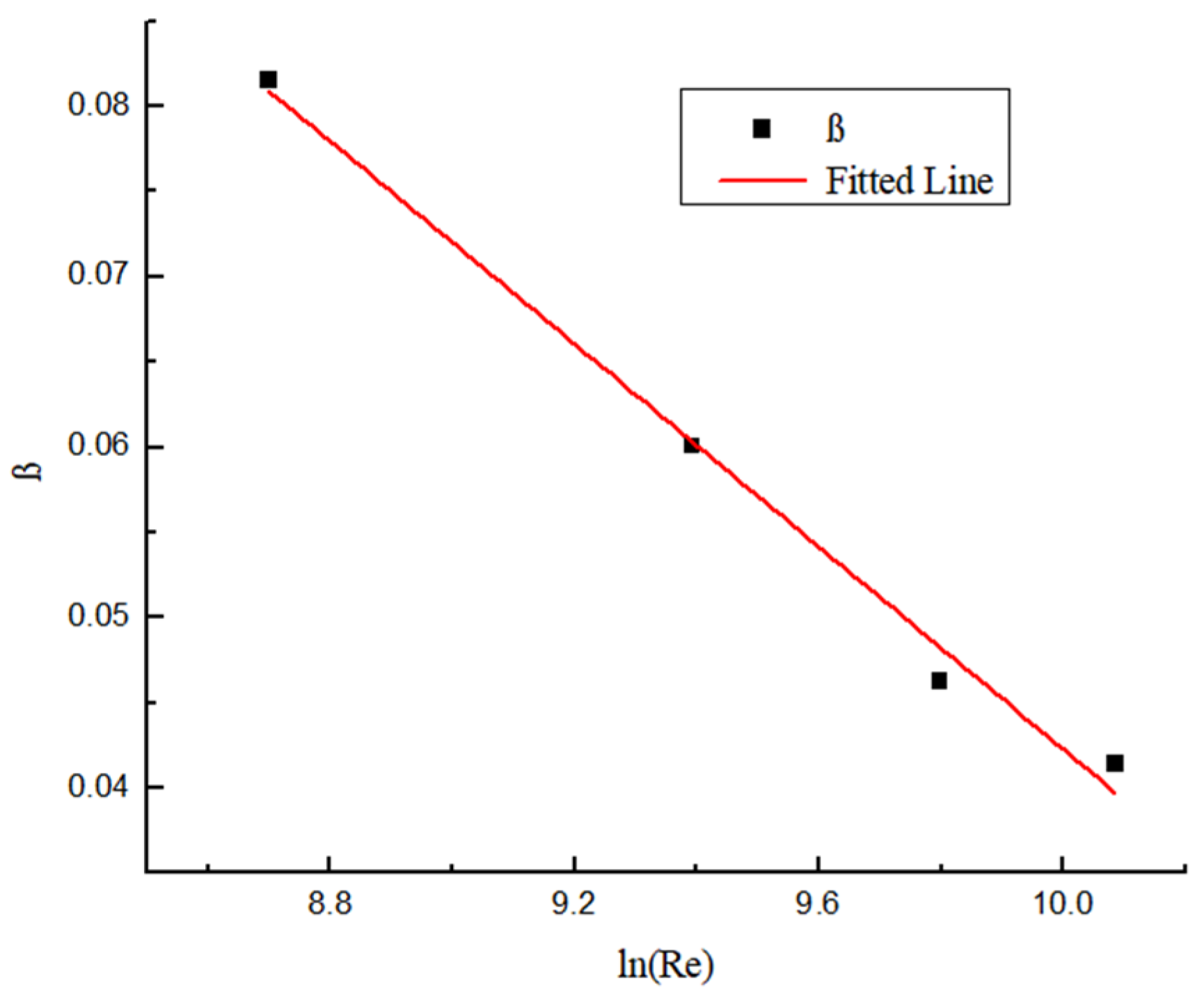
3.6. Attenuation Law of Swirl Number
3.7. Deposition Law of Hydrate Particles
4. Conclusions
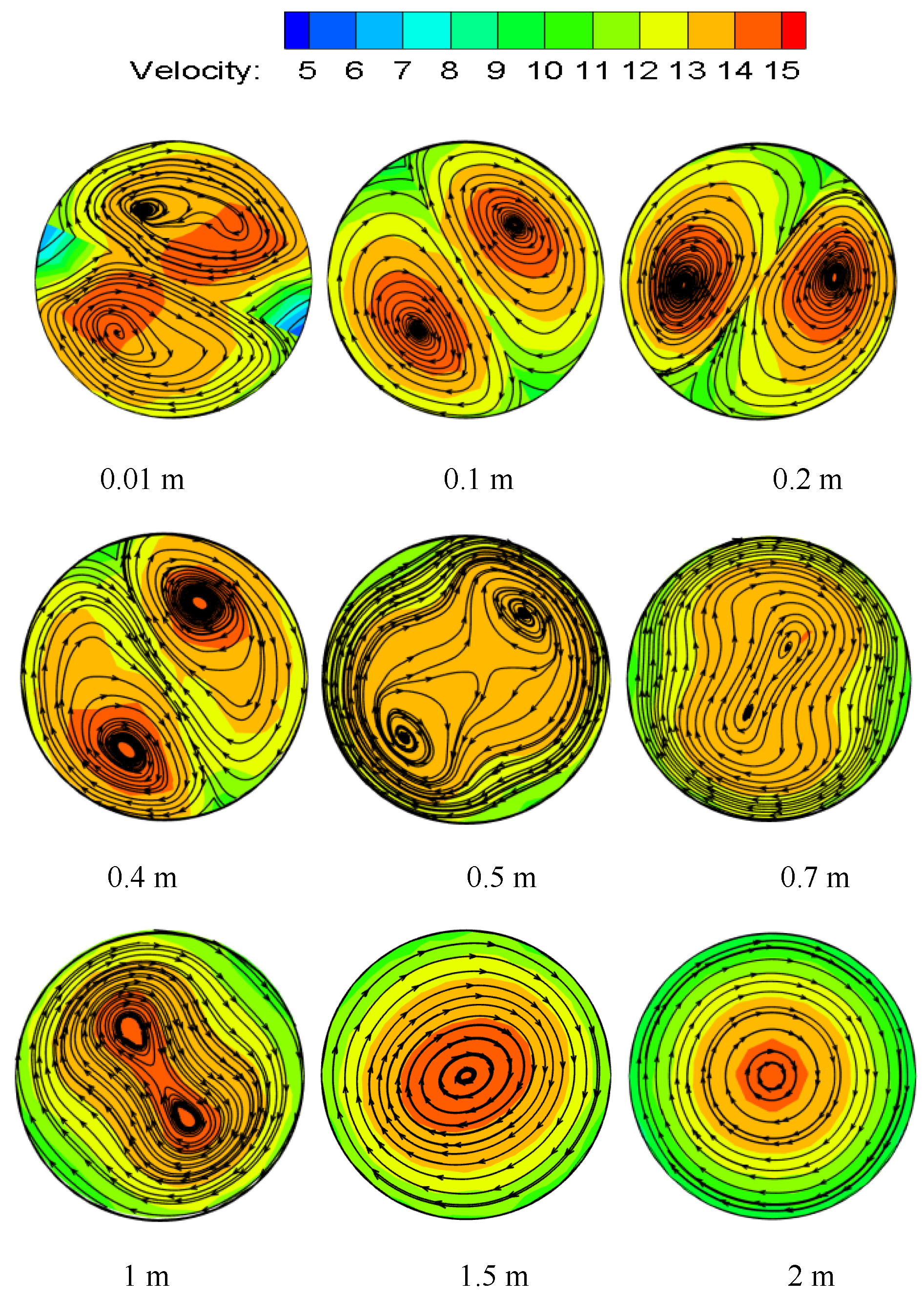
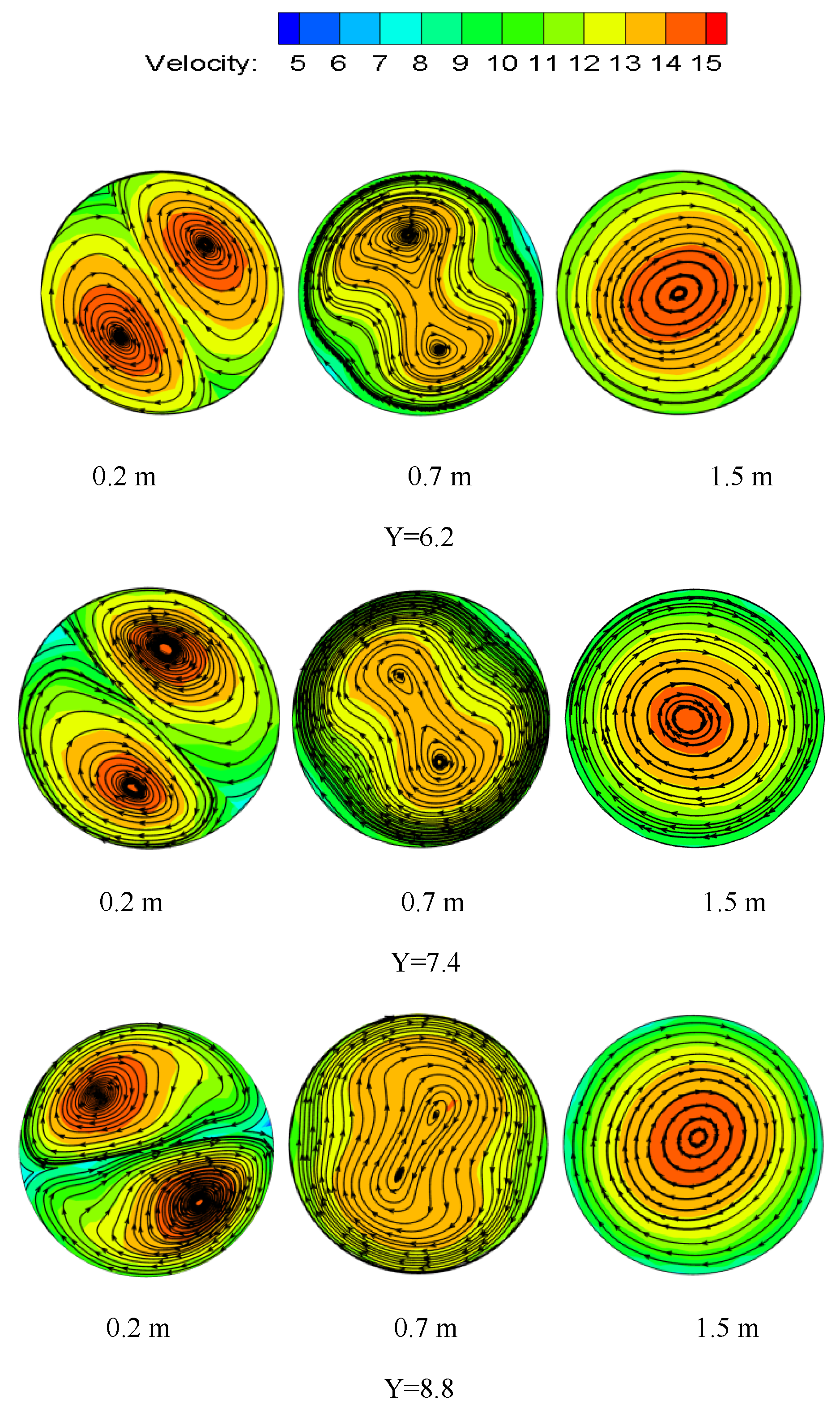
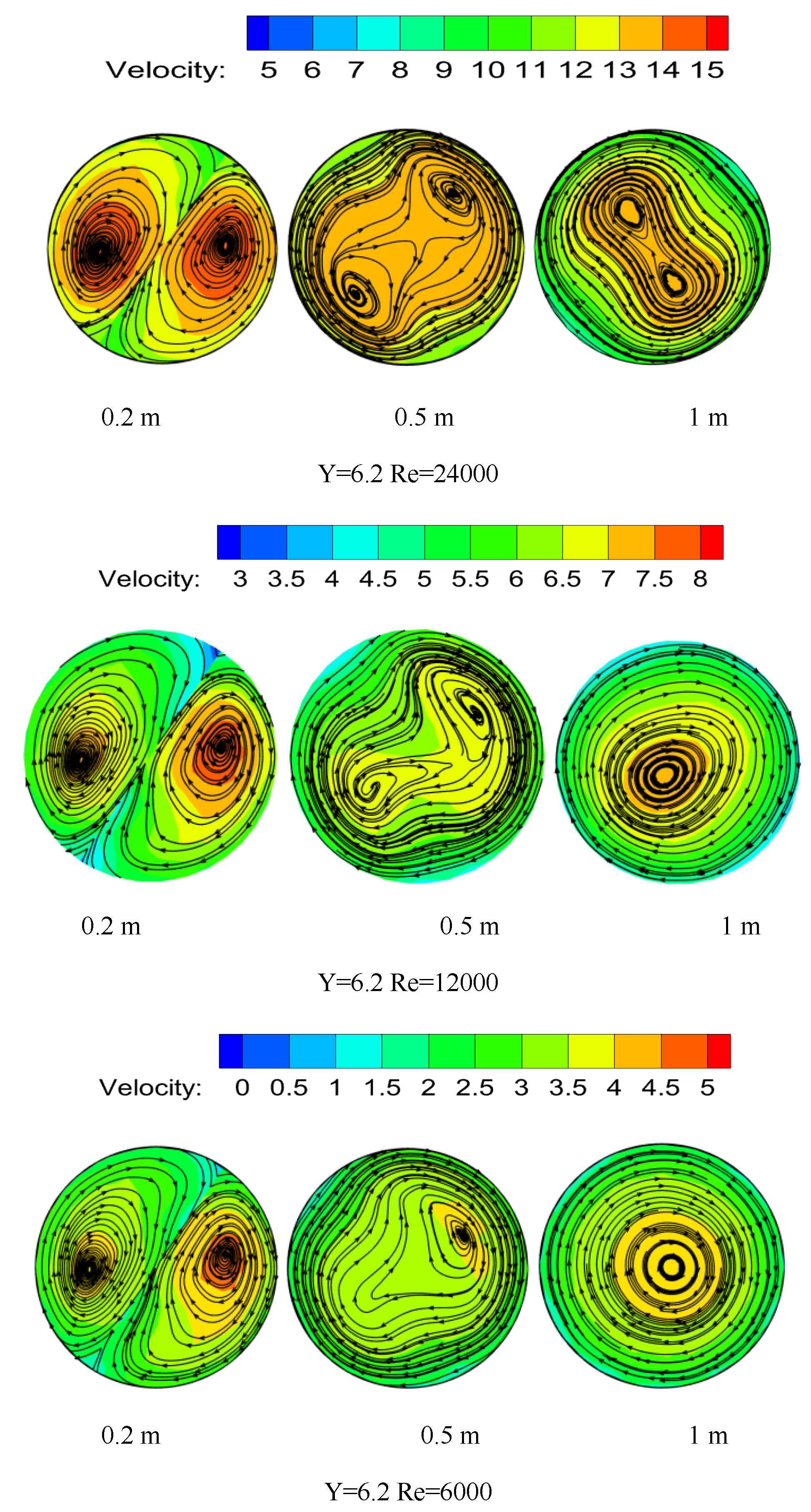
- The swirl flow velocity presents a symmetrical bimodal structure. The two velocity centers gradually move closer to the center of the pipeline and finally merge together with the attenuation of the swirl flow. The axial velocity is an “M” shape in the twisted segment, the peak value is 1/2r away from the pipeline wall, and the axial velocity is a parabolic shape in the rear pipeline segment. The absolute value of radial velocity is relatively small, which is the result of the redistribution of velocity by twisted band and it rapidly drops to 0 m/s in the posterior segment. The tangential velocity is the “M” shape in the twisted band section and the back pipe section. The peak value appears 1/6~1/7r away from the pipe wall.
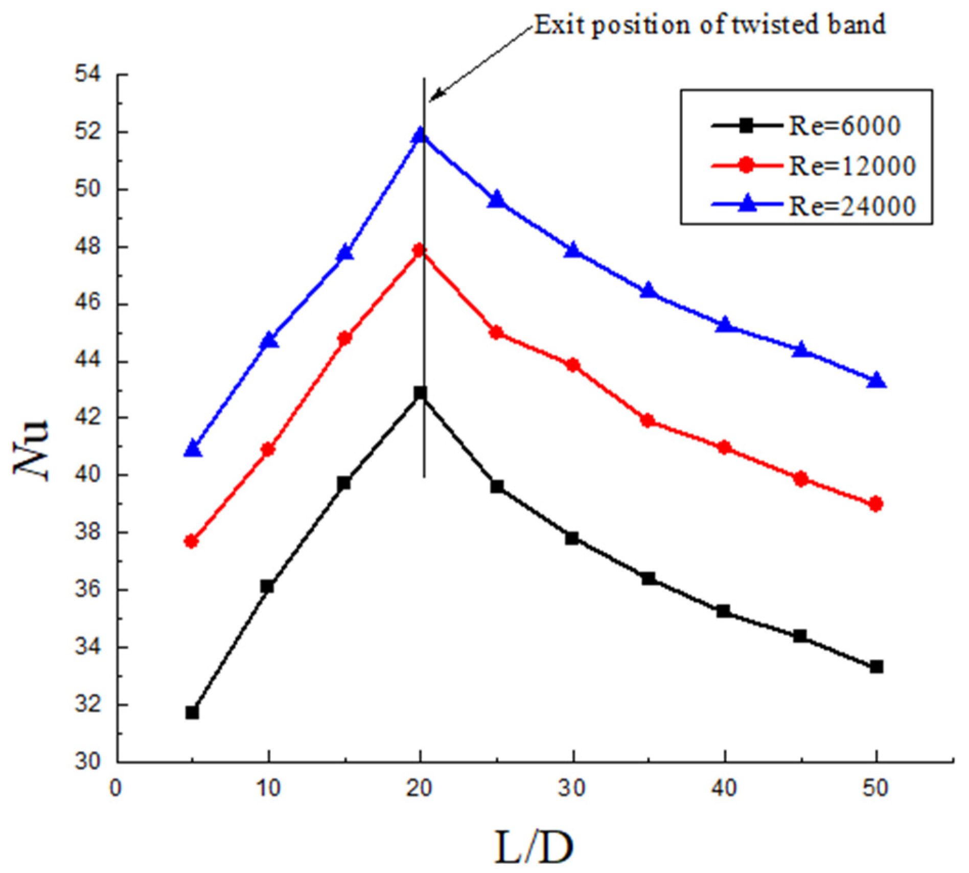
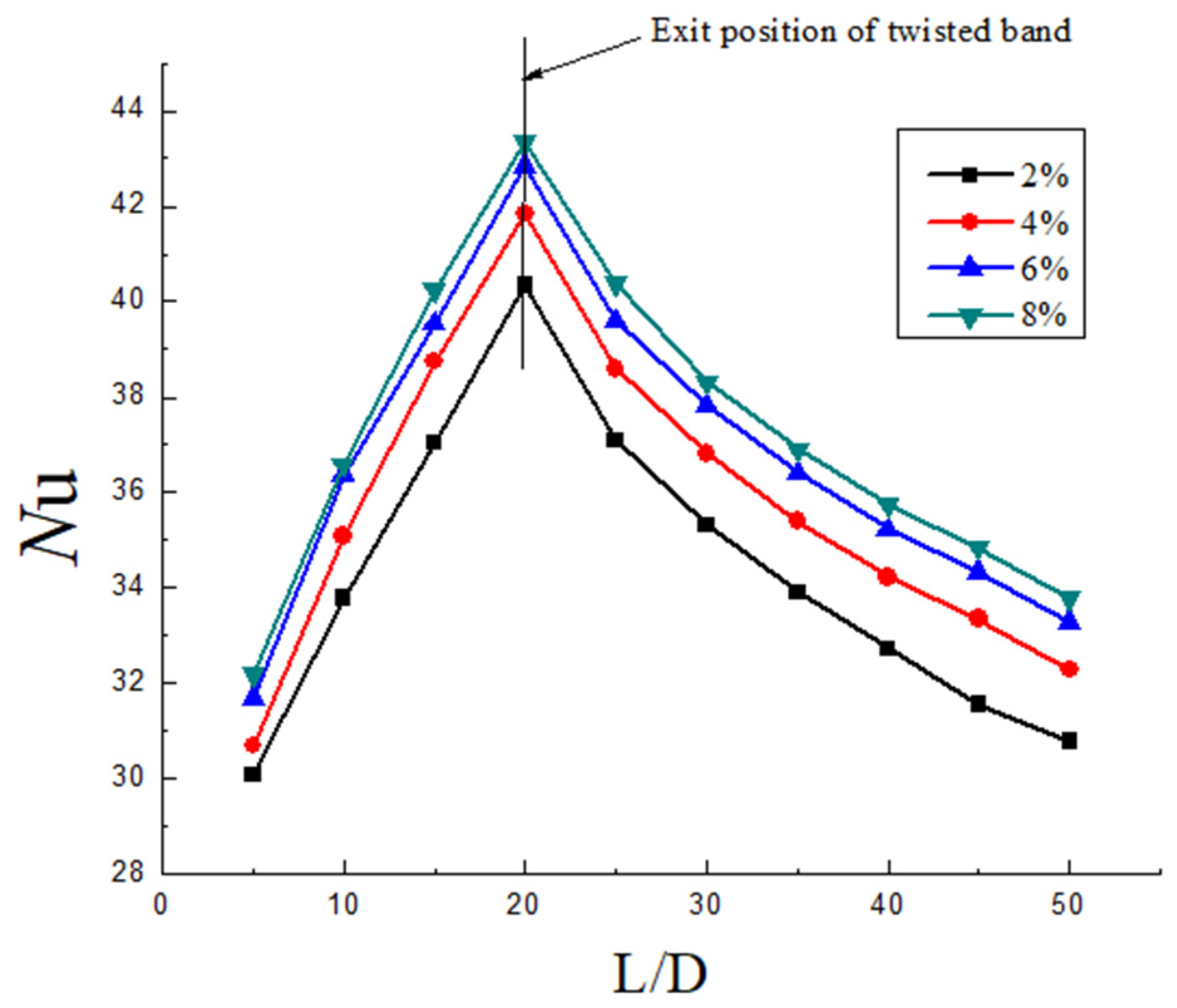
- Swirl flow can improve the heat transfer efficiency between the pipeline wall and the fluid, which is mainly related to Reynolds number, twist rate, and particle concentration. In the twisted band section, the Nu increases firstly, and it is removed after the twisted band. The Nu decreases and the slowing rate decreases continuously. The increase in Re has a more obvious induction effect on the motion of solid particles, thus Nu increases. With the increase in the volume fraction of particles, the increase rate of Nu number on the wall slows down. The twist rate is smaller, the Nu is larger, and the heat efficiency is higher.
- The turbulence intensity distribution in the twisted band section shows a “W” shape at the center of the rigid main vortex. The vortex in the free vortex area near the twisted band has a small scale and large unstable velocity pulsation, so the turbulence intensity is large. In the merging process of two symmetric vortexes outside the twisted band, the pulsation velocity at the central vortexes is increased, and the turbulence intensity distribution curve shows a “U” shape.
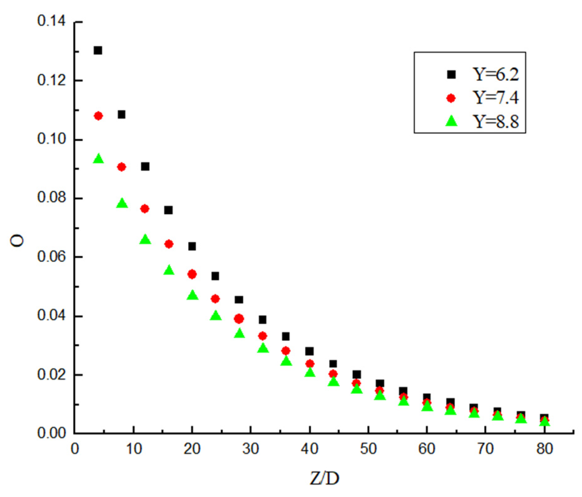
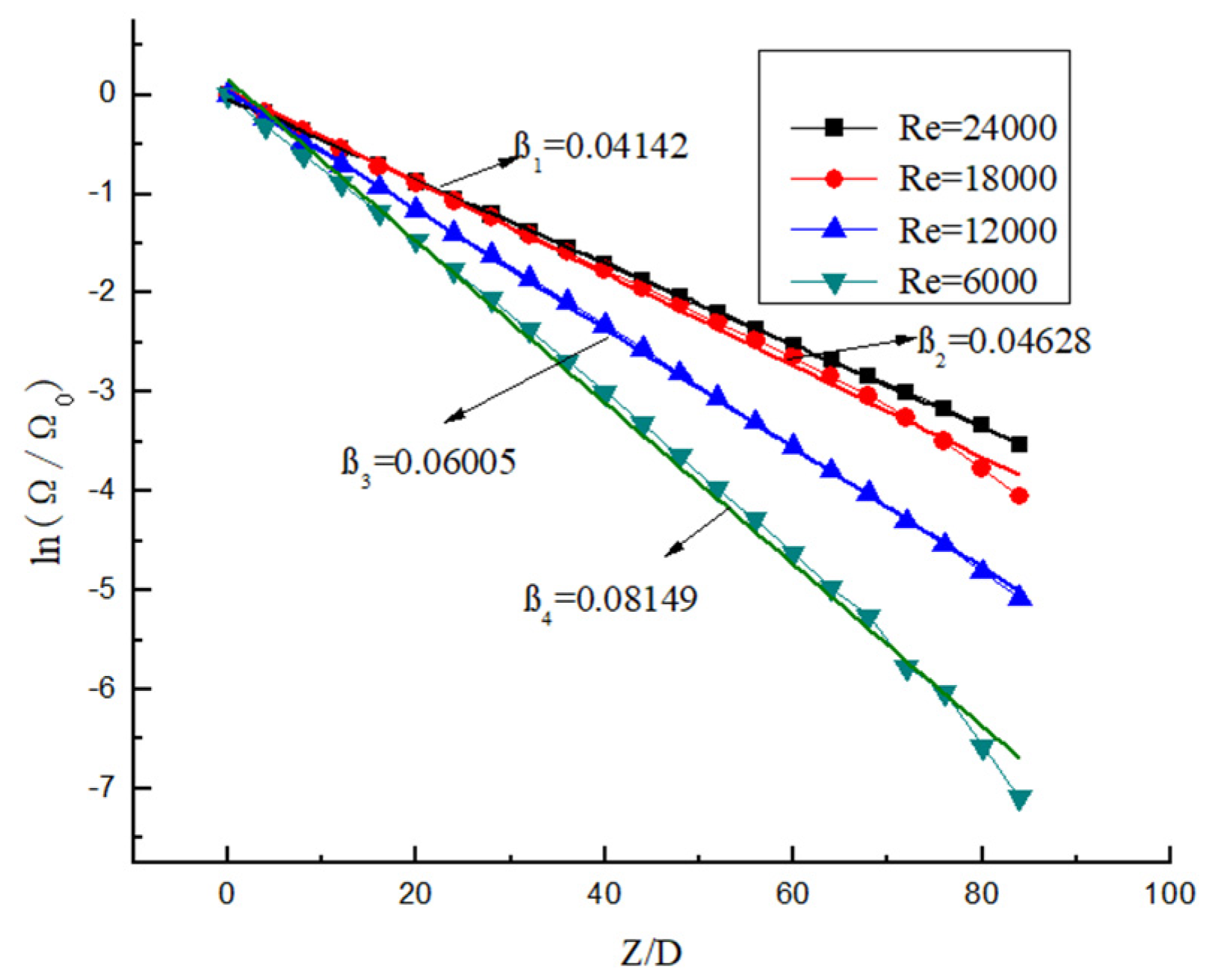
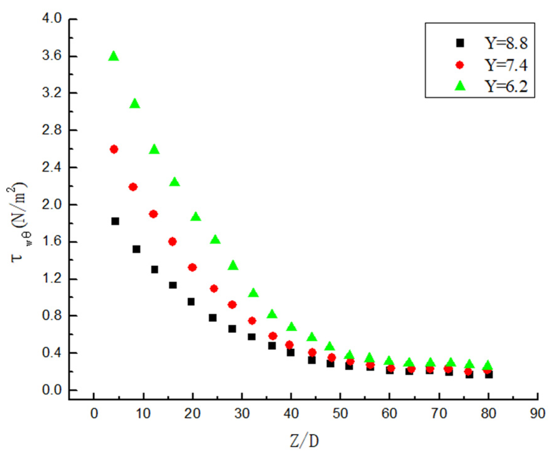
- The swirl direction of hydrate particles is the same as that of the twisted band. The vortex line swirl center begins to appear at both ends of the proximal twisted band, then it moves to the center of the proximal twisted band, and it finally moves to the edge of the pipeline to achieve stability. After leaving the twisted band, the vortex attenuates rapidly. The twist rate Y is smaller, the Re is larger, and the vortex attenuates more slowly. The attenuation rate of vorticity is mainly affected by Re, while the twist rate mainly affects the initial vorticity size. The shear stress is the main reason for the decrease in swirl strength, and the shear stress decreases exponentially in the pipe section with strong swirl flow. The twist rate mainly affects the initial swirl number, but it has little influence on the attenuation rate of swirl flow. The twist rate is smaller, the initial swirl number is larger. The attenuation of swirl flow is mainly related to Re, and the Re is larger, and it is slower. The swirl flow decreases exponentially, and the relation expression between swirl flow attenuation exponent and Re is obtained.
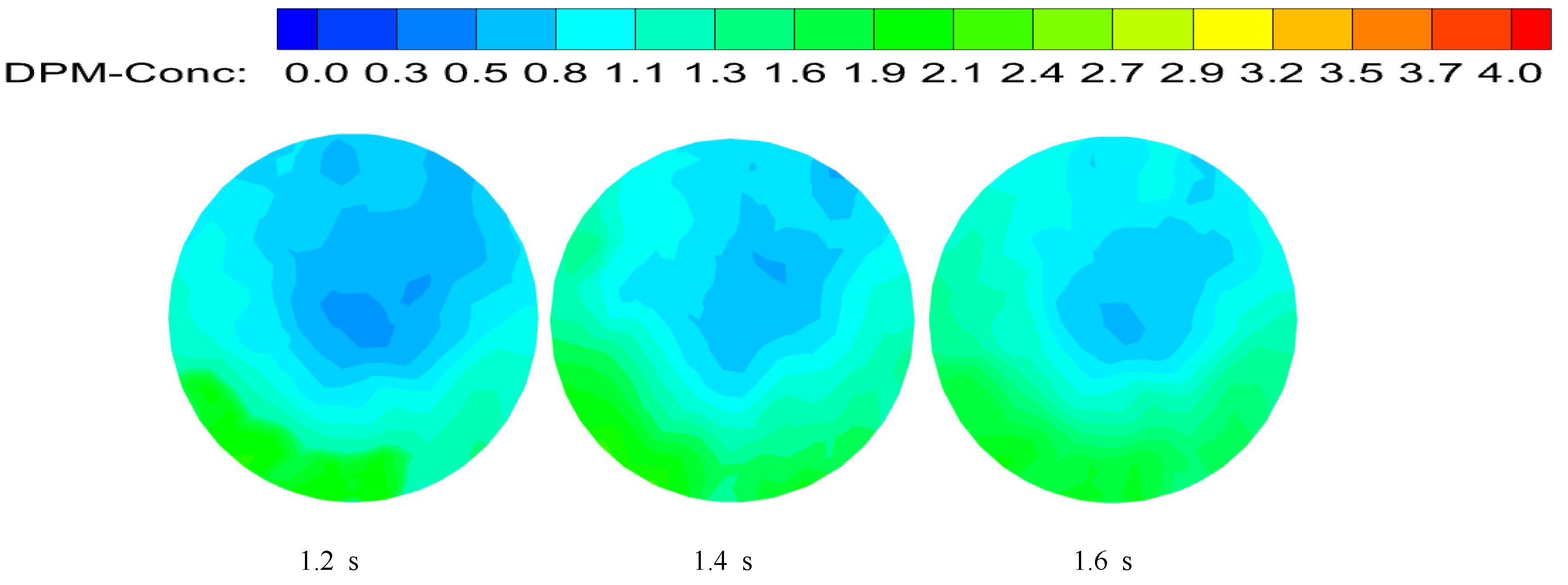
- The hydrate particles are distributed near the pipe wall under the action of centrifugal force generated by the swirl flow. The hydrate particles do not enter the forced vortex region. Due to the effect of shear force, the carrying distance of particles is increased. However, the swirl flow rapidly attenuates with the increase in carrying distance, the swirl radius of the particles decreases, and deposition occurs at the end of the pipe. The twist rate is larger, the swirl flow intensity is smaller, the attenuation is faster, and the particles are more likely to accumulate. In addition, the Re is larger, the cross-section particle distribution is more uniform, and the particle concentration is smaller.
Author Contributions
Funding
Data Availability Statement
Conflicts of Interest
References
- Sun, X. Experimental Research on the Hydraulic Characteristics and Particle Suspended Mechanics in Spiral Pipe Flow with Horizontal Axis. Ph.D. Thesis, Xi’an University of Technology, Xi’an, China, 2000. [Google Scholar]
- Zohir, A.E.; Aziz, A.A.A.; Habib, M.A. Heat transfer characteristics in a sudden expansion pipe equipped with swirl generators. Int. J. Heat Fluid Flow 2011, 32, 352–361. [Google Scholar] [CrossRef]
- Liu, W.; Cheng, X.; Chen, Y.; Bai, B. Gas-liquid two-phase cyclone field induced by spiral guide plate in tube. J. Mech. Eng. 2013, 49, 164–169. [Google Scholar] [CrossRef]
- Chen, B.; Ho, K.; Abakr, Y.A.; Chan, A. Fluid dynamics and heat transfer investigations of swirling decaying flow in an annular pipe Part 1: Review, problem description, verification and validation. Int. J. Heat Mass Transf. 2016, 97, 1029–1043. [Google Scholar] [CrossRef]
- Chen, B.; Ho, K.; Abakr, Y.A.; Chan, A. Fluid dynamics and heat transfer investigations of swirling decaying flow in an annular pipe Part 2: Fluid flow. Int. J. Heat Mass Transf. 1965, 97, 1012–1028. [Google Scholar] [CrossRef]
- Kreith, F.; Sonju, K. The decay of a turbulent swirl in a pipe. J. Fluid Mechine 1965, 22, 257–271. [Google Scholar] [CrossRef]
- Kitoh, O. Experimrntal study of turbluent swirling flow in a straight pipe. J. Fluid Mechine 1991, 225, 445–479. [Google Scholar] [CrossRef]
- Steenbergen, W.; Voskamp, J. The rate of decay of swirl in turbulent pipe flow. Flow Meas. Instrum. 1998, 9, 67–78. [Google Scholar] [CrossRef]
- Nanan, K.; Thianpong, C.; Promvonge, P.; Eiamsa-ard, S. Investigation of heat transfer enhancement by perforated swirl twisted-tapes. Int. Commun. Heat Mass Transf. 2014, 52, 106–112. [Google Scholar] [CrossRef]
- Bhuiya, M.M.K.; Chowdhury, M.S.U.; Shahabuddin, M.; Sahad, M.; Memone, L. Thermal characteristics in a heat exchanger pipeline fitted with triple twisted tape inserts. Int. Commun. Heat Mass Transf. 2013, 48, 124–132. [Google Scholar] [CrossRef]
- Najafi, A.F.; Mousavian, S.M.; Amini, K. Numerical investigations on swirl intensity decay rate for turbulent swirling flow in a fixed pipe. Int. J. Mech. Sci. 2011, 53, 801–811. [Google Scholar] [CrossRef]
- Chen, P.; Liu, F.; Li, Y.; Wang, W.; Liu, H.; Zhang, Q. Numerical simulation of flow characteristics of hydrate slurry. Oil Gas Storage Transp. 2014, 33, 160–164. [Google Scholar]
- Zhao, P. Study on the Plugging Mechanism and Flow Safety of Hydrate Slurry. Ph.D. Thesis, China University of Petroleum, Beijing, China, 2016. [Google Scholar]
- Song, G.; Li, Y.; Wang, W.; Zheng, S. Numerical simulation of hydrate particle size distribution characteristics in pipeline flowing systems. Chem. Ind. Eng. Prog. 2018, 8, 2312–2918. [Google Scholar]
- Guang, S.; Yu, L.; Wu, W.; Jiang, K.; Shi, Z.; Shu, Y. Numerical simulation of pipeline hydrate slurry flow behavior based on population balance theory. Chem. Ind. Eng. Prog. 2018, 2, 561–568. [Google Scholar]
- Liang, J.; Rao, Y.; Wang, S. Numerical Simulation of Spiral Flow and Heat Transfer of Gas-solid Two-phase Spiral Flow Generated by Twisted-tape. China Pet. Mach. 2018, 45, 109–116. [Google Scholar]
- Jun, L.; Yong, R.; Shu, W.; Shu, Z.; Zhou, S. Numerical Simulation of Spiral Flow and Heat Transfer of Hydrate Pipe Generated by Impeller. China Pet. Mach. 2018, 46, 120–126. [Google Scholar]
- Jassim, E.; Abdi, M.A.; Muzychka, Y. A new approach to investigate hydrate deposition in gas-dominated flowlines. J. Nat. Gas Sci. Eng. 2010, 2, 163–177. [Google Scholar] [CrossRef]
- Shi, X.J.; Zhang, P. Two-phase flow and heat transfer characteristics of tetra-n-butyl ammonium bromide clathrate hydrate slurry in horizontal 90elbow pipe and U-pipe. Int. J. Heat Mass Transf. 2016, 97, 364–378. [Google Scholar] [CrossRef]
- Boris, V.; Balakin, S.L.; Pawel, K.; Hoffmann, A.C. Modelling agglomeration and deposition of gas hydrates in industrial pipelines with combined CFD-PBM technique. Chem. Eng. Sci. 2016, 153, 45–57. [Google Scholar]
- Balakin, B.V.; Kosinska, A.; Kutsenko, K.V. Pressure drop in hydrate slurries: Rheology, granulometry and high water cut. Chem. Eng. Sci. 2018, 190, 77–85. [Google Scholar] [CrossRef]
- Song, G.; Li, Y.; Wang, W.; Jiang, K.; Shi, Z.; Yao, S. Investigation on the mechanical properties and mechanical stabilities of pipewall hydrate deposition by modelling and numerical simulation. Chem. Eng. Sci. 2018, 192, 477–487. [Google Scholar] [CrossRef]
- Li, P.; Zhang, X.; Lu, X. Three-dimensional Eulerian modeling of gas–liquid–solid flow with gas hydrate dissociation in a vertical pipe. Chem. Eng. Sci. 2018, 53, 1–19. [Google Scholar] [CrossRef]
- Ziyad, S.K.Y.; Kumar, A. Numerical investigation of isothermal and non-isothermal ice slurry flow in horizontal elliptical pipes. Int. J. Refrig. 2019, 97, 196–210. [Google Scholar]
- He, X.; Wang, S.; Liu, F. A method for accurately calculating the density of natural gas hydrate. Nat. Gas Ind. 2004, 24, 30–31. [Google Scholar]
- Sari, O.; Vuarnoz, D.; Meili, F.; Peter, E. Visualization of ice slurries and ice slurry flows. In Proceedings of the Second Workshop on Ice Slurries of the International Instistute of Refrigeration, Paris, France, 25–26 May 2000. [Google Scholar]
- Kitanovski, A.; Vuarnoz, D.; Ata-Caesar, D.; Egolf, P.W.; Hansen, T.M.; Doetsch, C. The fluid dynamics of ice slurry. Int. J. Refrig. 2005, 28, 37–50. [Google Scholar] [CrossRef]
- Wang, S.; Rao, Y.; Zhang, L.; Ma, W.; Zhao, S. Research Situation and Progress on Flow Characteristics of Spiral Flow in Horizontal Pipe. J. Taiyuan Univ. Technol. 2013, 44, 232–236. [Google Scholar]


| Particle Concentration (%) | Particle Size (mm) | Twist rate Y | Initial Velocity (m/s) |
|---|---|---|---|
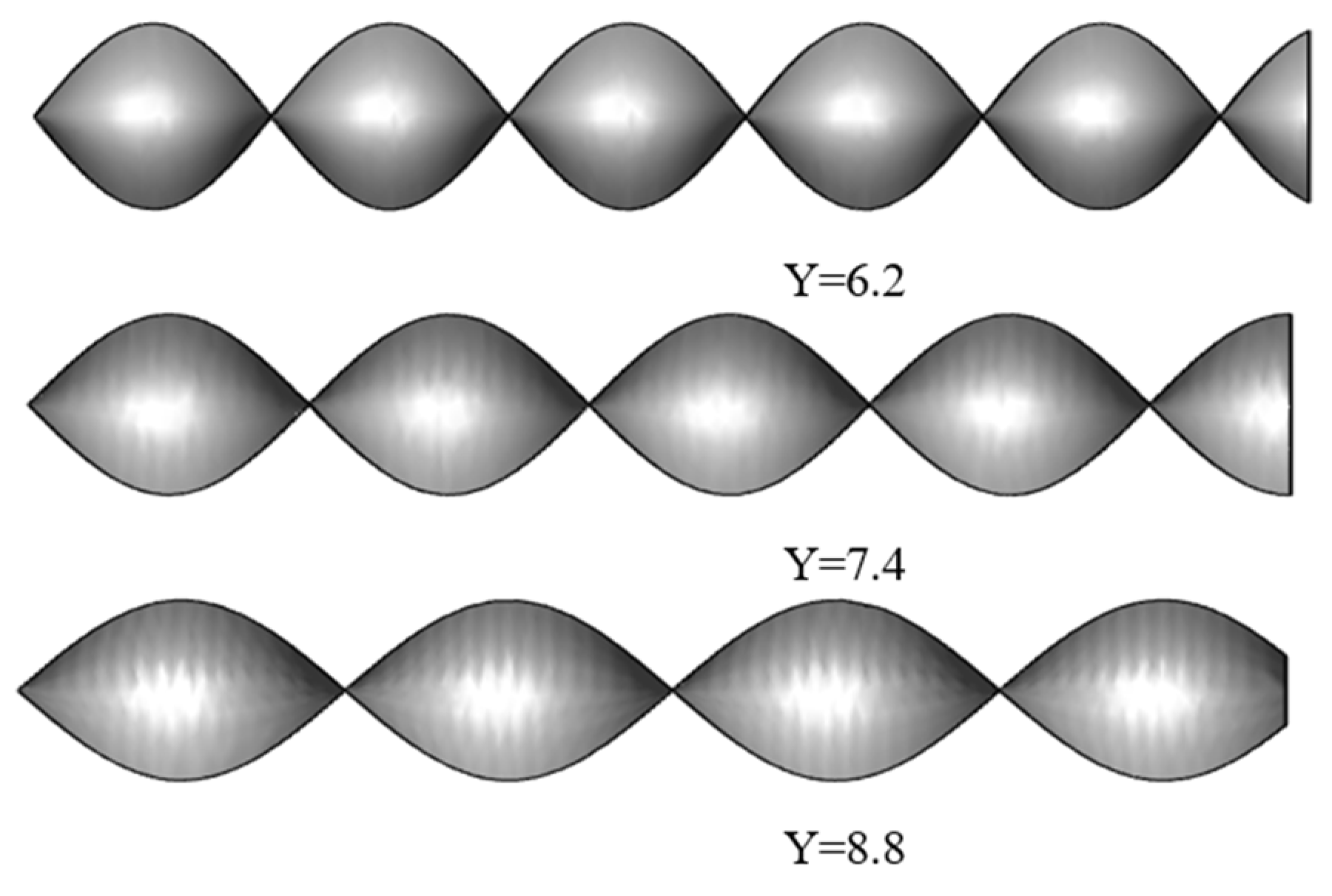
| 1~8 | 0.001 | 6.2/7.4/8.8 | 0.5~12 |
Publisher’s Note: MDPI stays neutral with regard to jurisdictional claims in published maps and institutional affiliations. |
© 2021 by the authors. Licensee MDPI, Basel, Switzerland. This article is an open access article distributed under the terms and conditions of the Creative Commons Attribution (CC BY) license (https://creativecommons.org/licenses/by/4.0/).
Share and Cite
Rao, Y.; Liu, Z.; Wang, S.; Li, L.; Sun, Q. Numerical Simulation of Swirl Flow Characteristics of CO2 Hydrate Slurry by Short Twisted Band. Entropy 2021, 23, 913. https://doi.org/10.3390/e23070913
Rao Y, Liu Z, Wang S, Li L, Sun Q. Numerical Simulation of Swirl Flow Characteristics of CO2 Hydrate Slurry by Short Twisted Band. Entropy. 2021; 23(7):913. https://doi.org/10.3390/e23070913
Chicago/Turabian StyleRao, Yongchao, Zehui Liu, Shuli Wang, Lijun Li, and Qi Sun. 2021. "Numerical Simulation of Swirl Flow Characteristics of CO2 Hydrate Slurry by Short Twisted Band" Entropy 23, no. 7: 913. https://doi.org/10.3390/e23070913
APA StyleRao, Y., Liu, Z., Wang, S., Li, L., & Sun, Q. (2021). Numerical Simulation of Swirl Flow Characteristics of CO2 Hydrate Slurry by Short Twisted Band. Entropy, 23(7), 913. https://doi.org/10.3390/e23070913