
Financial Return Distributions: Past, Present, and COVID-19


Abstract
1. Introduction
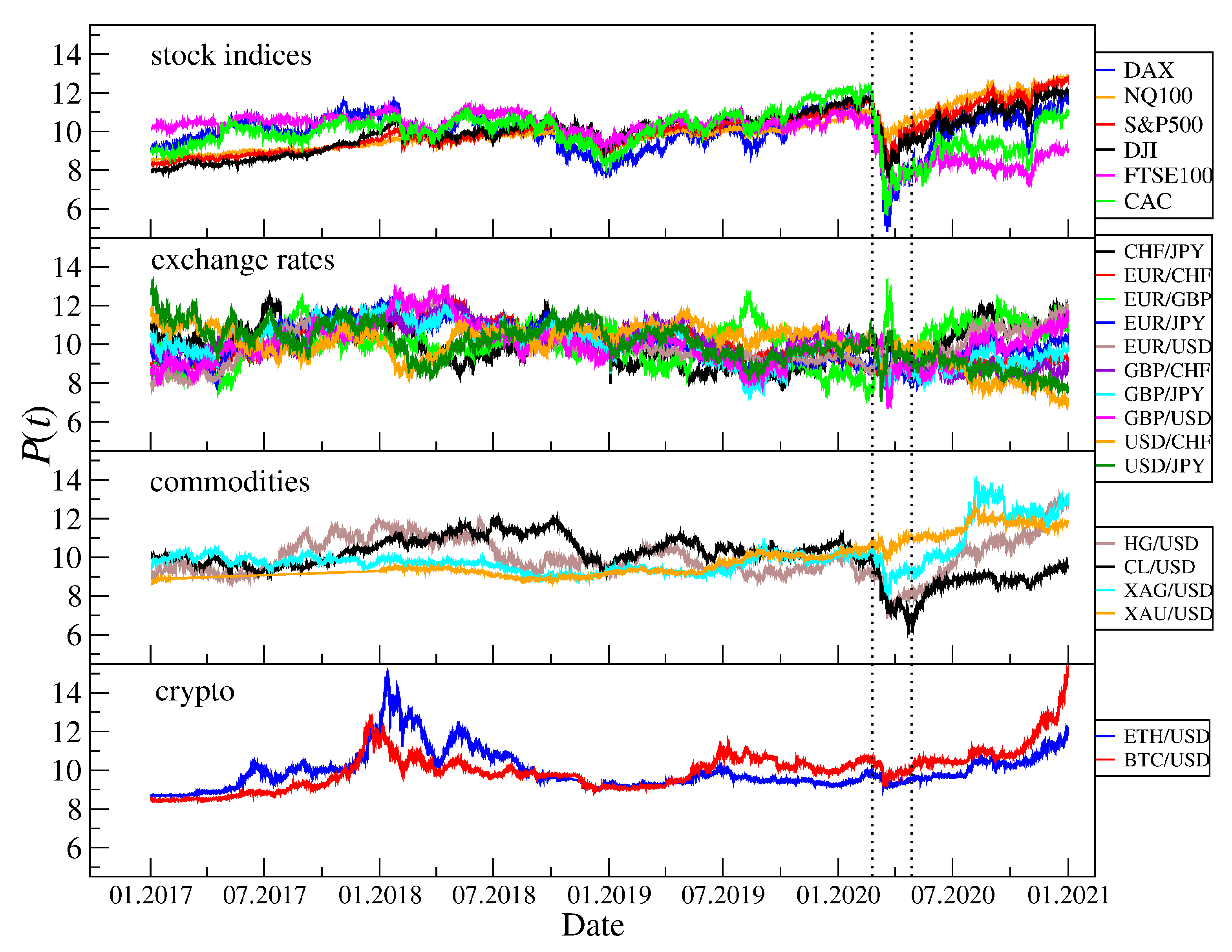
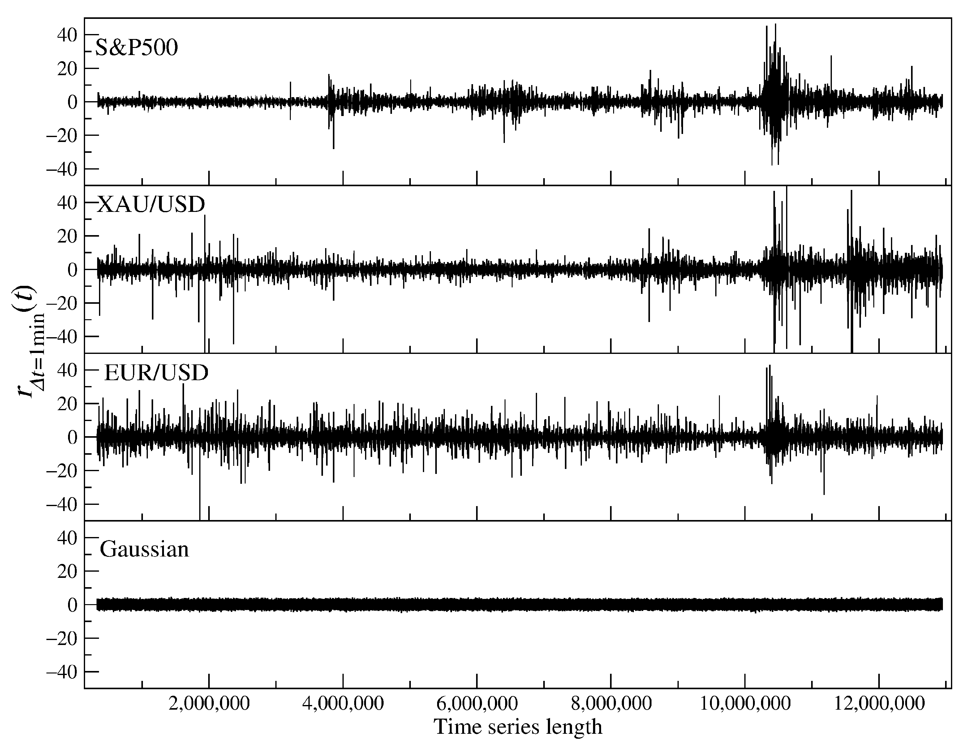
2. Data
3. Results
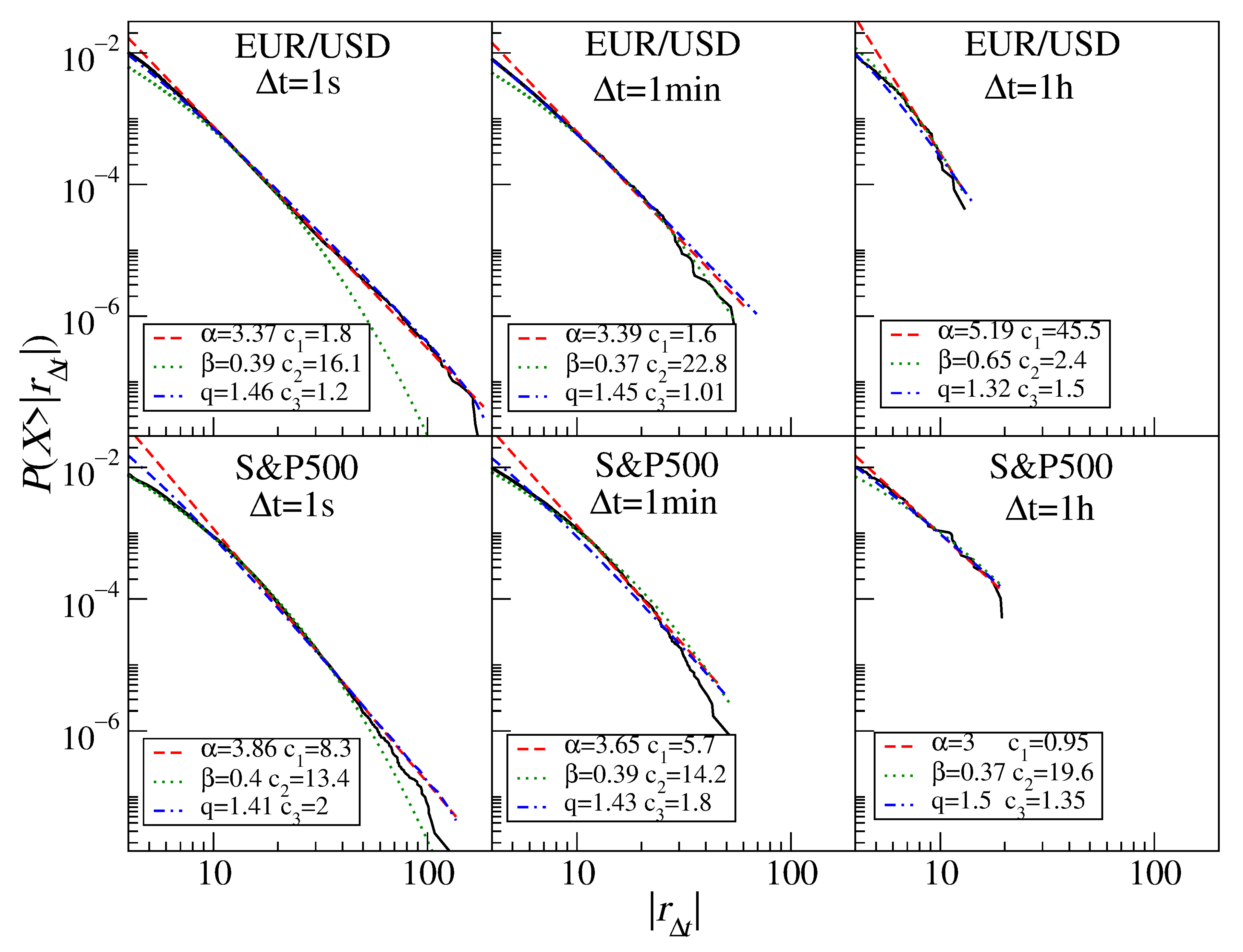
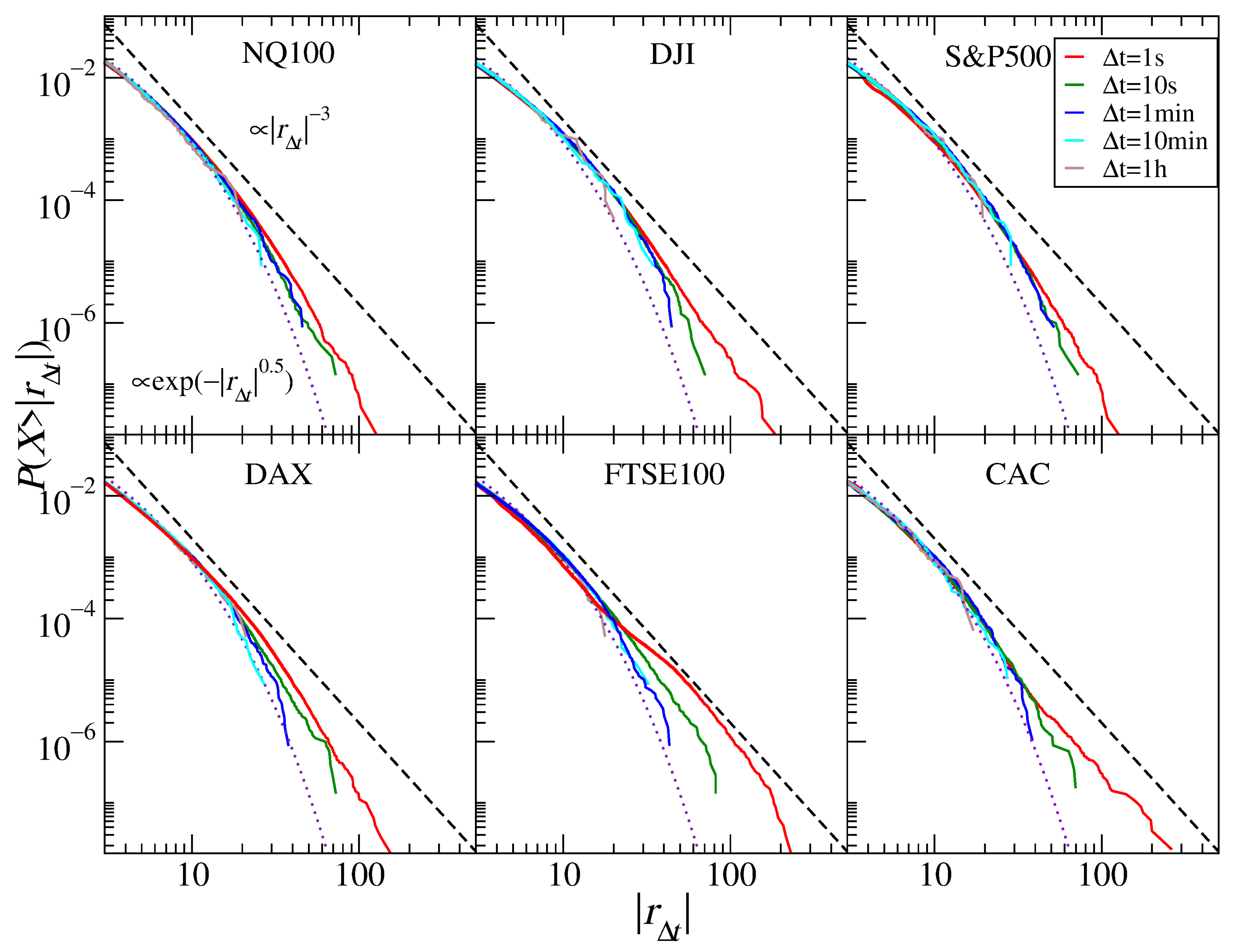
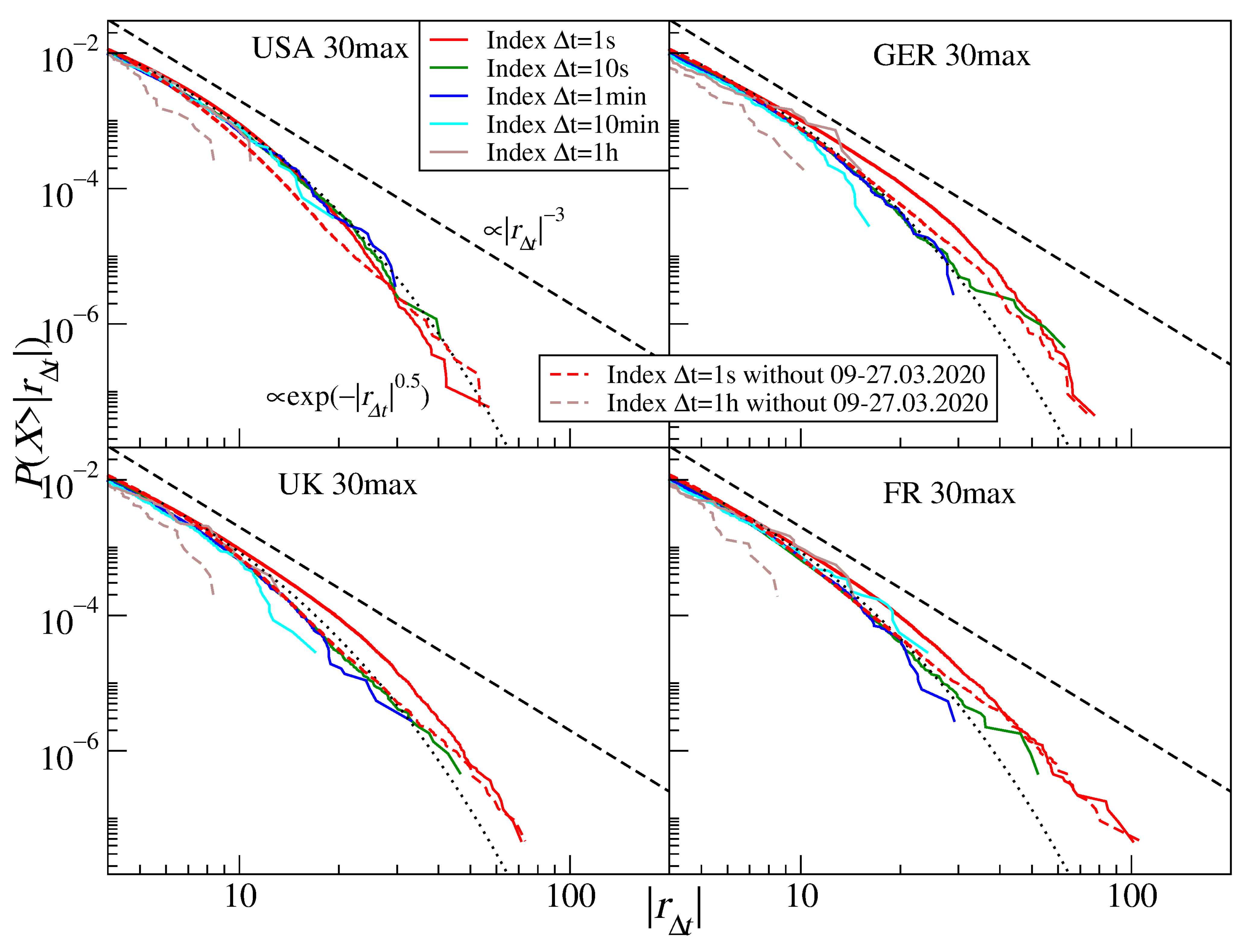
3.1. Stock Market Indices
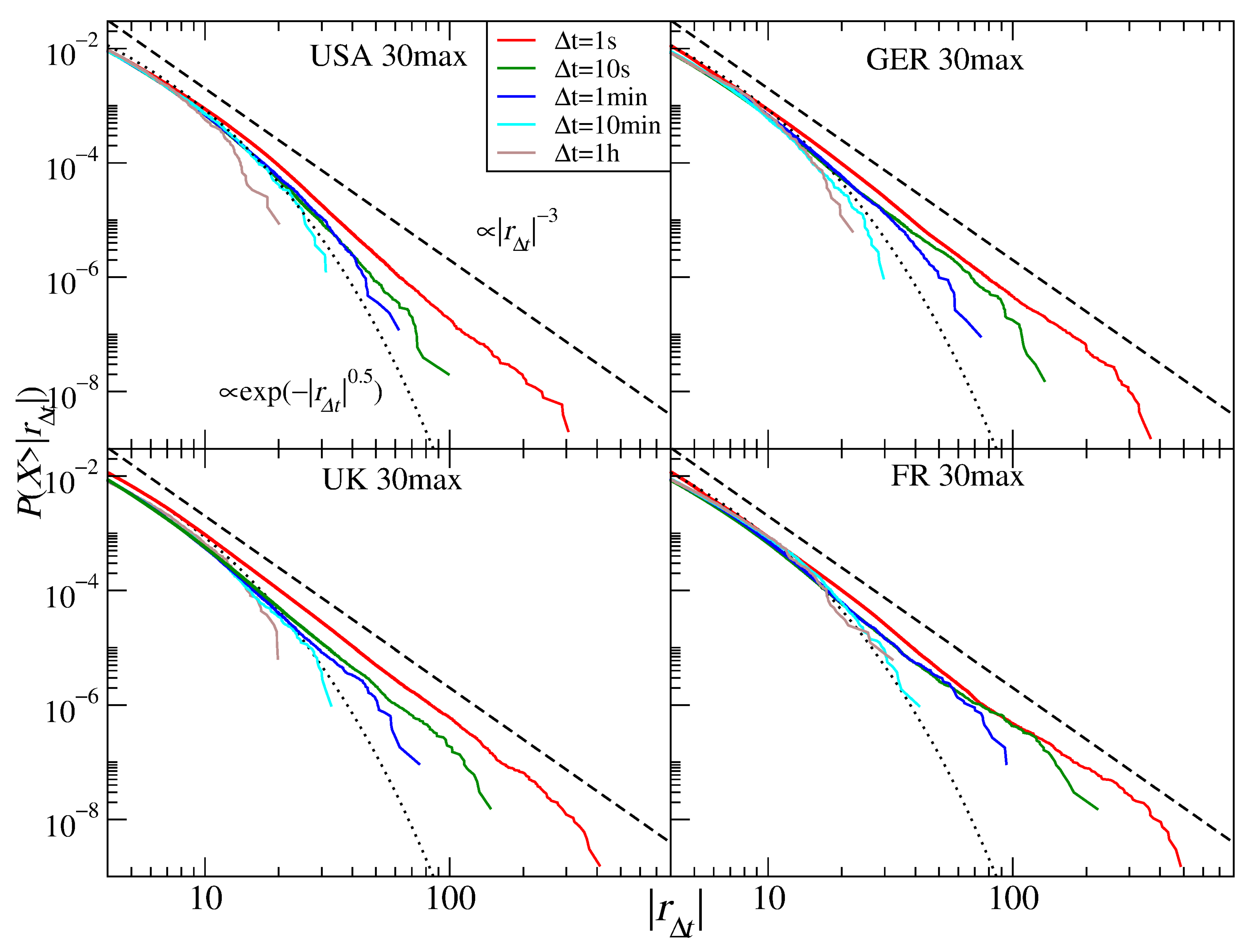
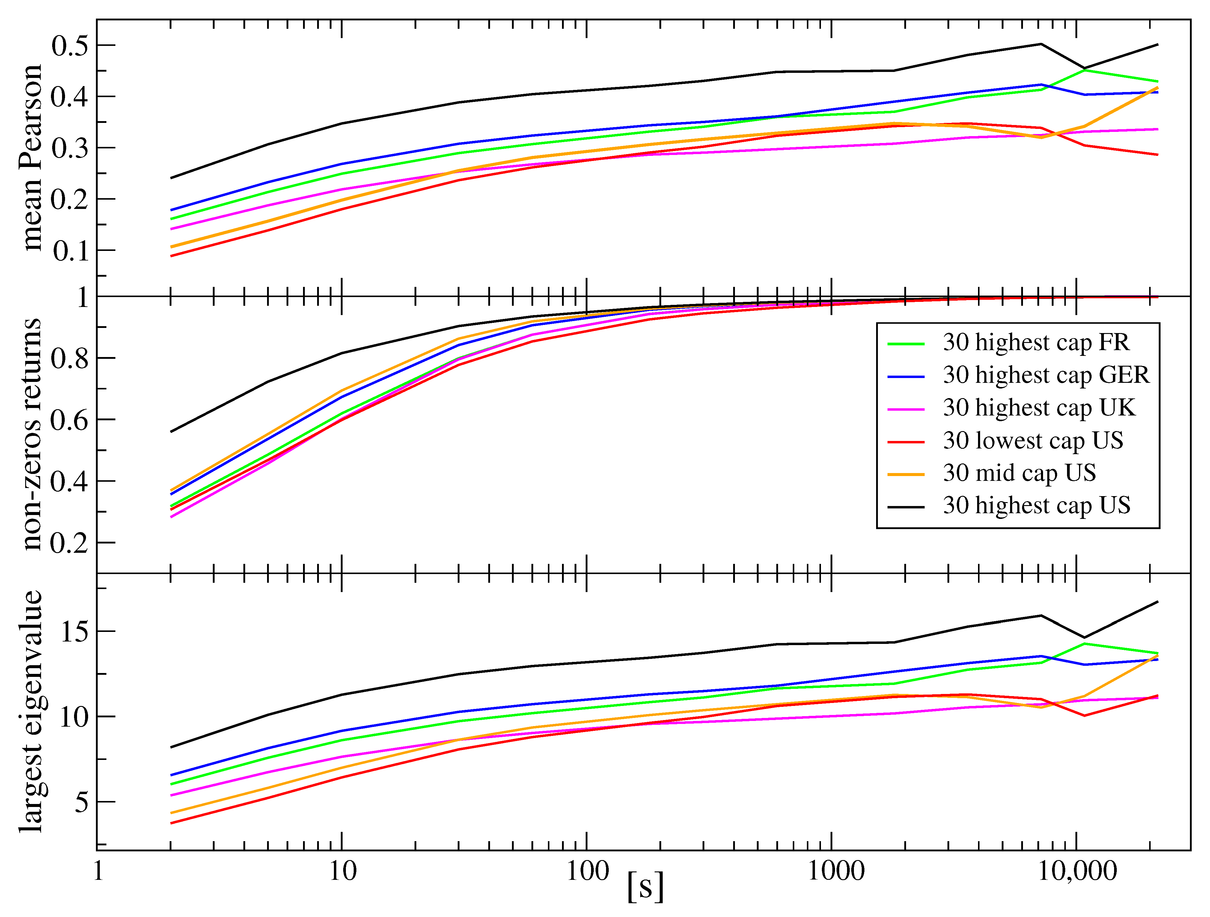
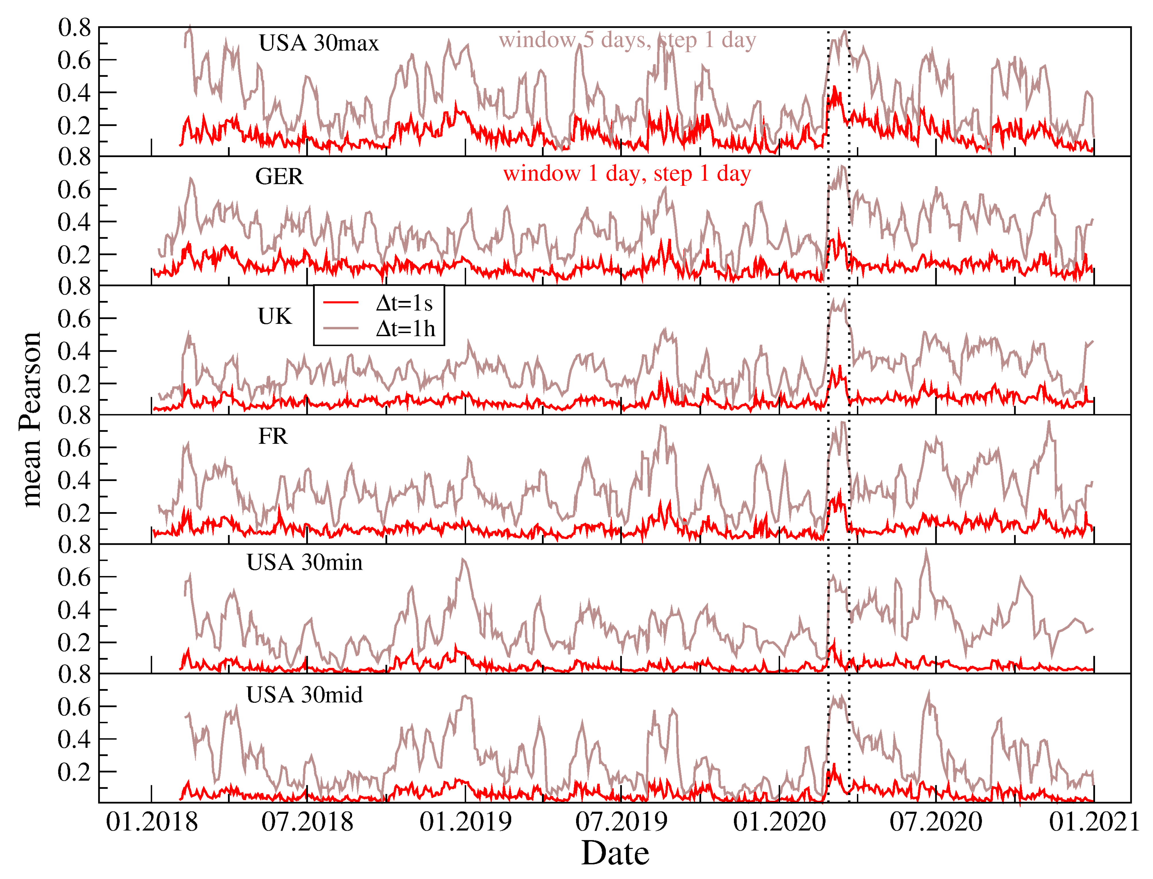
3.2. Individual Stocks
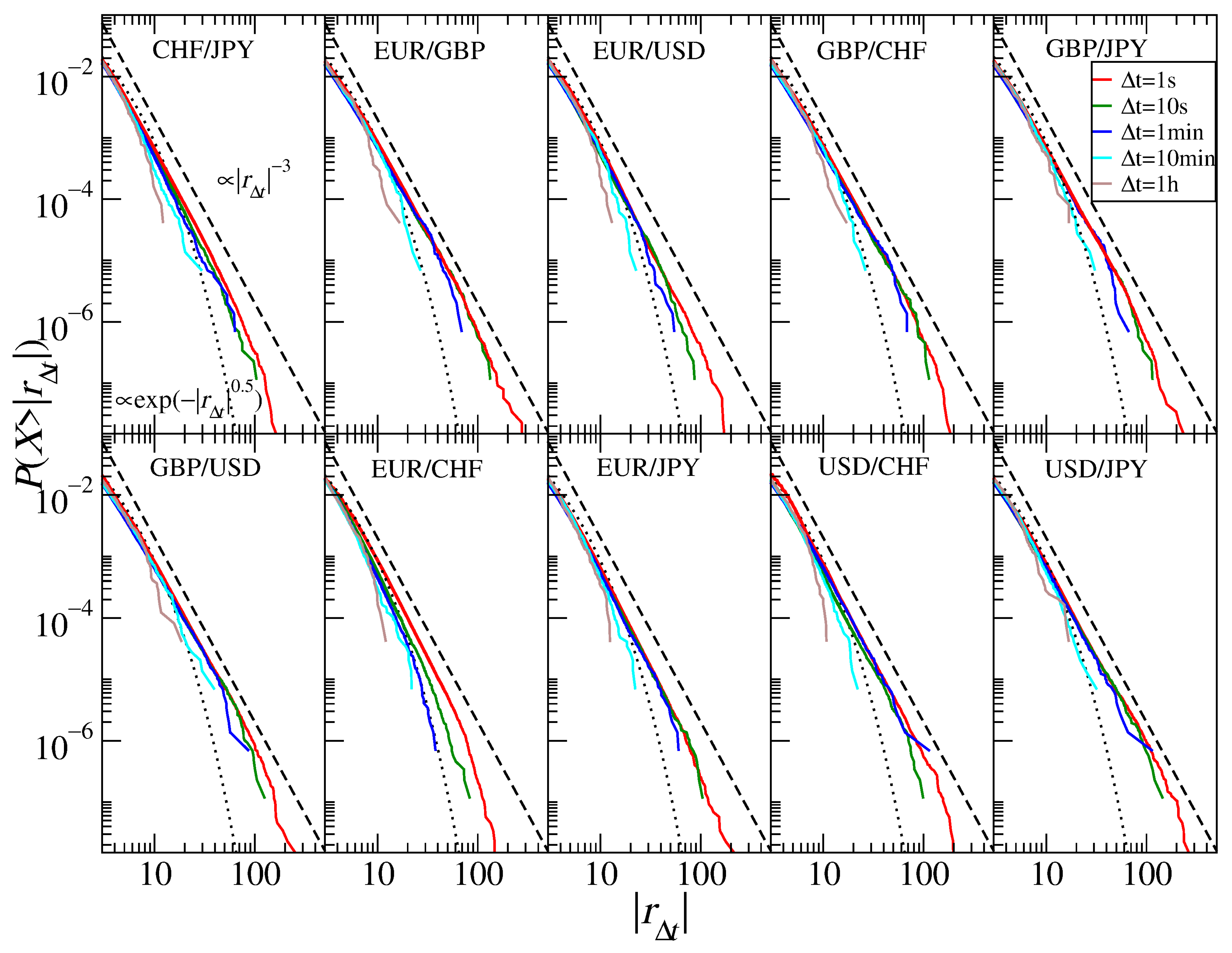
3.3. Currencies
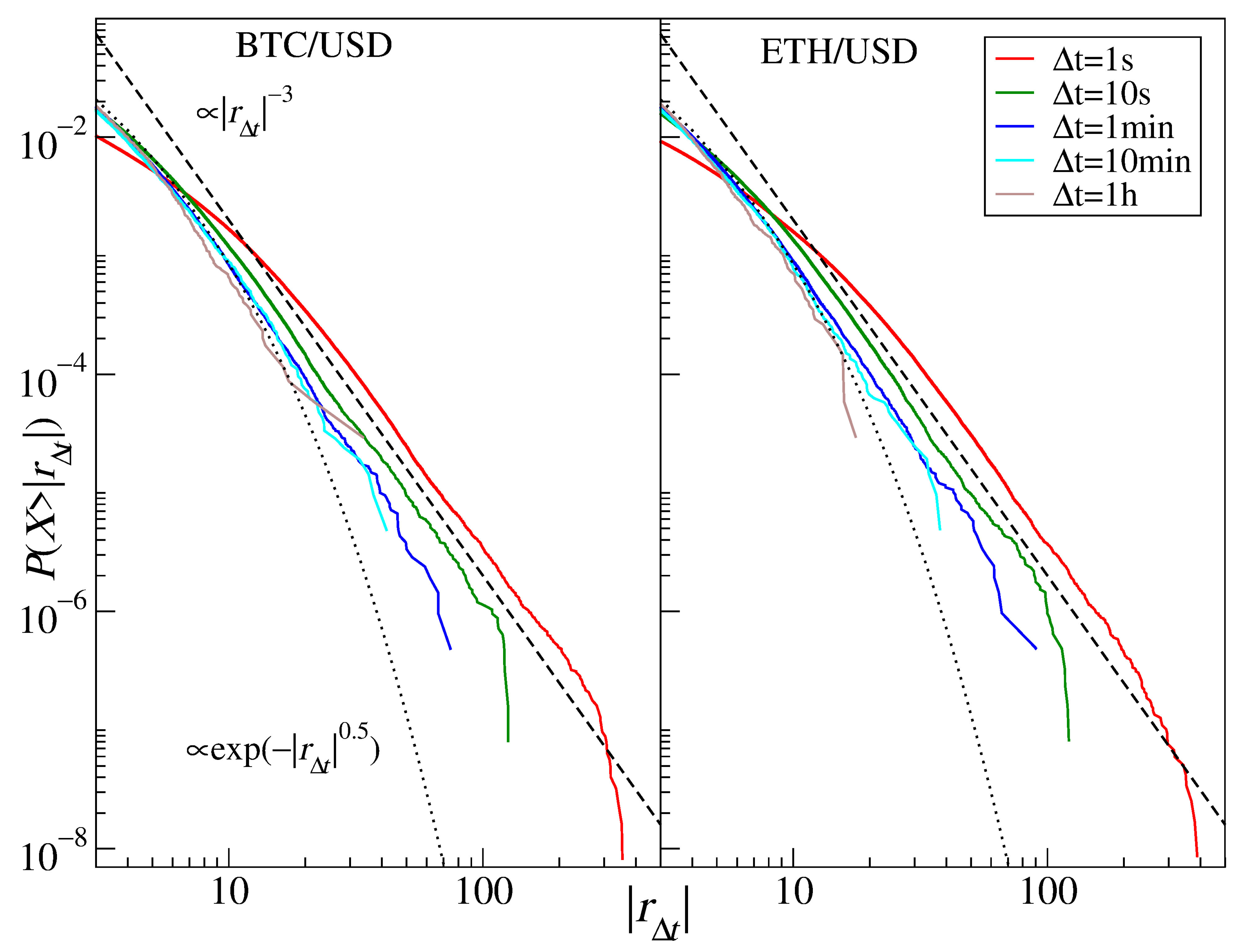
3.4. Cryptocurrencies
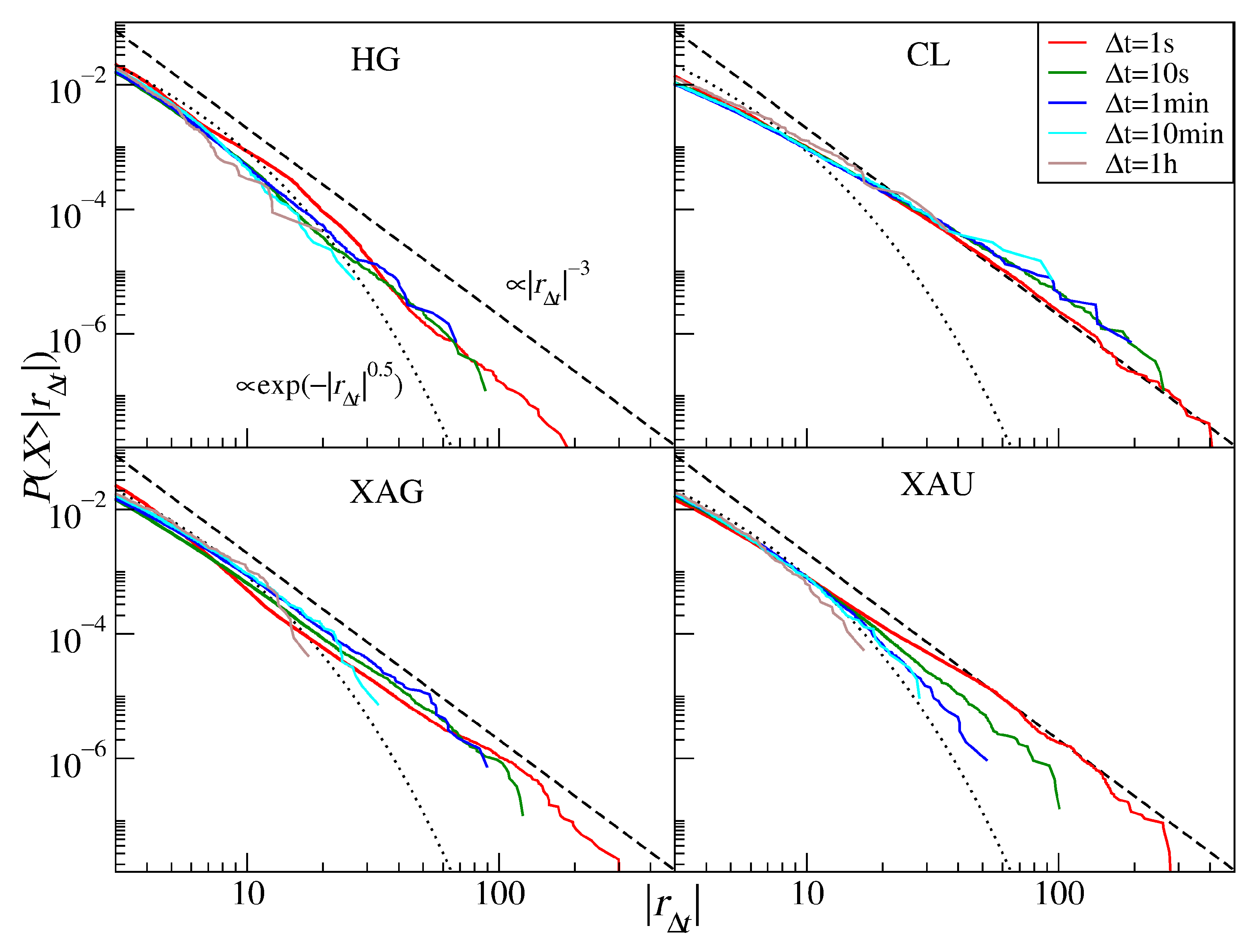
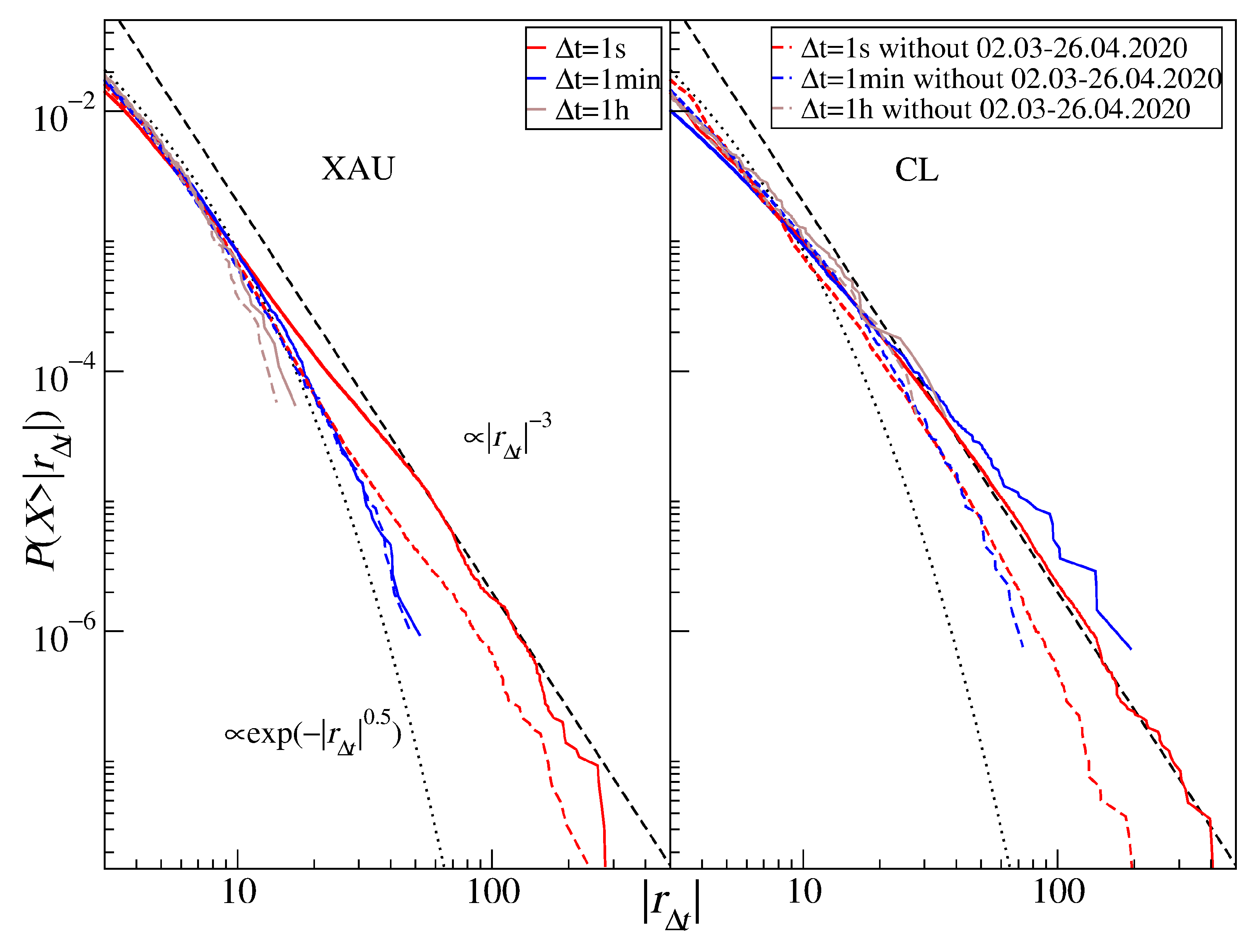
3.5. Commodities
4. Summary
Author Contributions
Funding
Institutional Review Board Statement
Informed Consent Statement
Data Availability Statement
Conflicts of Interest
Appendix A

| U.S. Large | U.S. Medium | U.S. Small | U.K. Large | German Large | French Large | ||||||
|---|---|---|---|---|---|---|---|---|---|---|---|
| Ticker | USD | Ticker | USD | Ticker | USD | Ticker | GBP | Ticker | EUR | Ticker | EUR |
| AAPL | 2000 | BIDU | 68.6 | CAG | 18.7 | RDSB | 107.4 | VOW3 | 140.6 | VK | 330.9 |
| MSFT | 1784 | NSC | 68.1 | MGM | 18.4 | ULVR | 105.7 | SAP | 126 | MC | 288 |
| AMZN | 1537 | CL | 67.7 | CAH | 18.3 | AZN | 94.2 | SIE | 112.5 | OR | 181.3 |
| GOOGL | 1378 | SHW | 67 | CTL | 18.1 | RIO | 88.7 | ALV | 89.5 | SAN | 105.2 |
| FB | 805 | SO | 65.9 | ULTA | 17.6 | HSBA | 86.4 | DTE | 81.8 | FP | 102.8 |
| BABA | 625 | APD | 63.1 | OMC | 16.3 | DGE | 70.4 | DAI | 80.6 | AIR | 78.9 |
| BRKB | 593 | ICE | 62.6 | TIF | 16 | BATS | 62.3 | BAS | 65.3 | KER | 74.8 |
| TSM | 592.8 | D | 60.9 | DVN | 14.8 | BP | 59 | MRK | 62.3 | SU | 73.8 |
| TSLA | 582 | ADSK | 59.5 | AAL | 14.7 | RB | 46.3 | DPW | 57.6 | AI | 65.9 |
| JPM | 473 | ADI | 56.6 | WYNN | 14.5 | BLT | 44.2 | BMW | 57.3 | BNP | 65.1 |
| V | 458 | ILMN | 56.2 | WHR | 14.1 | PRU | 40.6 | VNA | 56.7 | CS | 54.9 |
| JNJ | 438.5 | PGR | 55.9 | L | 13.8 | AAL | 39.5 | ADS | 52.8 | SAF | 51 |
| WMT | 383.5 | VRTX | 55.8 | SJM | 13.7 | GLEN | 38.1 | BAYN | 52.3 | DG | 50.8 |
| MA | 360 | BSX | 54.8 | TEVA | 12.7 | VOD | 37.7 | IFX | 47.6 | RI | 42.1 |
| UNH | 358.2 | EMR | 54.7 | IPG | 11.5 | REL | 35.5 | HEN3 | 38.5 | BN | 37.8 |
| DIS | 337 | NOC | 53.7 | DVA | 11.5 | LSE | 35.3 | MUV2 | 37 | ACA | 36.3 |
| PG | 336 | HUM | 53.3 | NWL | 11.4 | BARC | 31.7 | PAH3 | 28.7 | EDF | 35.4 |
| BAC | 331 | MET | 53.1 | GPS | 11.3 | NG | 30.7 | DB1 | 26 | VIV | 30.4 |
| HD | 324 | PBR | 53 | TAP | 11.3 | LLOY | 30.3 | EOAN | 26 | ENGI | 29.3 |
| NVDA | 318 | REGN | 51 | CF | 9.7 | CPG | 26.7 | RWE | 23.2 | ORA | 27.8 |
| PYPL | 277 | TWTR | 50 | NRG | 9.2 | CRH | 26.3 | CON | 22.8 | SGO | 26.8 |
| INTC | 261 | KHC | 49.9 | KSS | 9.1 | EXPN | 23.4 | DBK | 21.2 | CAP | 24.9 |
| CMCSA | 252.6 | NEM | 49.8 | MRO | 8.7 | RBS | 22.4 | FRE | 20.9 | LR | 21.3 |
| XOM | 243 | F | 49 | X | 6.9 | AHT | 20.1 | BEI | 20.5 | UG | 19.4 |
| VZ | 243 | DG | 48.6 | MAT | 6.9 | WOS | 20.1 | FME | 18.4 | GLE | 19.2 |
| KO | 231.6 | ITUB | 48.4 | APA | 6.8 | ABF | 19.4 | HEI | 15.3 | ALO | 16.2 |
| NFLX | 228 | MAR | 48 | AA | 6.1 | CCL | 18.1 | TKA | 7.1 | EN | 13 |
| ADBE | 224 | FCX | 47.7 | JWN | 6 | TSCO | 17.6 | CBK | 6.6 | PUB | 12.7 |
| CSCO | 222 | KMB | 47 | M | 5.1 | LGEN | 16.9 | LHA | 6.6 | VIE | 12.6 |
| T | 217.9 | LVS | 46.8 | EQT | 5.1 | ANTO | 16.7 | LXS | 5.5 | CA | 12.3 |
References
- Bachelier, L. Théorie de spéculation. Ann. Sci. l’Ecole Norm. Supér. 1900, 3, 21–86. [Google Scholar] [CrossRef]
- Lévy, P. Calcul des Probabilités; Gauthier-Villars: Paris, France, 1925. [Google Scholar]
- Paul, W.; Baschnagel, J. Stochastic Processes: From Physics to Finance; Springer: Berlin/Heidelberg, Germany, 1999. [Google Scholar]
- Mandelbrot, B.B. The variation of certain speculative prices. J. Bus. 1963, 36, 394–419. [Google Scholar] [CrossRef]
- Fama, E.F. The behavior of stock-market prices. J. Bus. 1965, 38, 404–419. [Google Scholar] [CrossRef]
- Blume, M.E. Portfolio theory: A step towards its practical application. J. Bus. 1970, 43, 152–173. [Google Scholar] [CrossRef]
- Teichmoeller, J. A note on the distribution of stock price changes. J. Am. Stat. Assoc. 1970, 66, 282–284. [Google Scholar] [CrossRef]
- Blattberg, R.C.; Gonedes, N.J. A comparison of the stable and Student distributions as statistical models for stock prices. J. Bus. 1974, 47, 245–280. [Google Scholar] [CrossRef]
- Officer, R.R. The distribution of stock returns. J. Am. Stat. Assoc. 1972, 67, 807–812. [Google Scholar] [CrossRef]
- Barnea, A.; Downes, D.H. A reexamination of the empirical distribution of stock price changes. J. Am. Stat. Assoc. 1973, 68, 348–350. [Google Scholar] [CrossRef]
- Young, M.S.; Graff, R.A. Real estate is not normal: A fresh look at real estate return distributions. J. Real Estate Financ. Econ. 1995, 10, 225–259. [Google Scholar] [CrossRef]
- Clark, P.K. A subordinated stochastic process model with finite variance for speculative prices. Econometrica 1973, 41, 135–155. [Google Scholar] [CrossRef]
- Engle, R.F. Autoregressive conditional heteroscedasticity with estimates of the variance of United Kingdom inflation. Econometrica 1982, 50, 987–1007. [Google Scholar] [CrossRef]
- Mantegna, R.N.; Stanley, H.E. Scaling behaviour in the dynamics of an economic index. Nature 1995, 376, 46–49. [Google Scholar] [CrossRef]
- Couto Miranda, L.; Riera, R. Truncated Lévy walks and an emerging market economic index. Phys. A Stat. Mech. Appl. 2003, 297, 509–520. [Google Scholar] [CrossRef]
- Plerou, V.; Gopikrishnan, P.; Amaral, L.A.N.; Meyer, M.; Stanley, H.E. Scaling of the distribution of price fluctuations of individual companies. Phys. Rev. E 1999, 60, 6519–6529. [Google Scholar] [CrossRef] [PubMed]
- Gopikrishnan, P.; Plerou, V.; Amaral, L.A.N.; Meyer, M.; Stanley, H.E. Scaling of the distribution of fluctuations of financial market indices. Phys. Rev. E 1999, 60, 5305–5316. [Google Scholar] [CrossRef] [PubMed]
- Gopikrishnan, P.; Meyer, M.; Amaral, L.A.N.; Stanley, H.E. Inverse cubic law for the distribution of stock price variations. Eur. Phys. J. B 1998, 3, 139–140. [Google Scholar] [CrossRef]
- Lux, T. The stable Paretian hypothesis and the frequency of large returns: An examination of major German stocks. Appl. Financ. Econ. 1996, 6, 463–475. [Google Scholar] [CrossRef]
- Makowiec, D.; Gnaciński, P. Fluctuations of WIG-the index of Warsaw Stock Exchange. Preliminary studies. Acta Phys. Pol. B 2001, 32, 1487–1500. [Google Scholar]
- Drożdż, S.; Kwapień, J.; Grümmer, F.; Ruf, F.; Speth, J. Quantifying the dynamics of financial correlations. Phys. A Stat. Mech. Appl. 2001, 299, 144–153. [Google Scholar] [CrossRef]
- Lillo, F.; Bonanno, G.; Mantegna, R.N. Variety of stock returns in normal and extreme market days: The August 1998 crisis. In Empirical Science of Financial Fluctuations; Takayasu, H., Ed.; Springer: Berlin/Heidelberg, Germany, 2002; pp. 77–89. [Google Scholar]
- Kaizoji, T.; Bornholdt, S.; Fujiwara, Y. Dynamics of price and trading volume in a spin model of stock markets with heterogeneous agents. Phys. A Stat. Mech. Appl. 2002, 316, 441–452. [Google Scholar] [CrossRef]
- Drożdż, S.; Kwapień, J.; Grümmer, F.; Ruf, F.; Speth, J. Are the contemporary financial fluctuations sooner converging to normal? Acta Phys. Pol. B 2003, 34, 4293–4306. [Google Scholar]
- Kim, K.; Yoon, S.-M. Dynamical behavior of continuous tick data in futures exchange market. Fractals 2003, 11, 131–136. [Google Scholar] [CrossRef]
- Kim, K.; Yoon, S.-M.; Kim, Y. Herd behaviors in the stock and foreign exchange markets. Phys. A Stat. Mech. Appl. 2004, 341, 526–532. [Google Scholar] [CrossRef][Green Version]
- Coronel-Brizio, H.F.; Hernándex-Montoya, A.R. On fitting the Pareto–Lévy distribution to stock market index data: Selecting a suitable cutoff value. Phys. A Stat. Mech. Appl. 2005, 354, 437–449. [Google Scholar] [CrossRef]
- Sinha, S.; Pan, R.K. The power (law) of Indian markets: Analysing NSE and BSE trading statistics. In Econophysics of Stock and Other Markets. Proc. Econophys-Kolkata II; Chatterjee, A., Chakrabarti, B.K., Eds.; Springer: Berlin/Heidelberg, Germany, 2006. [Google Scholar]
- Oh, G.; Kim, S.; Um, C.-J. Statistical properties of the returns of stock prices of international markets. arXiv 2006, arXiv:physics/0601126. [Google Scholar]
- Rak, R.; Drożdż, S.; Kwapień, J. Nonextensive statistical features of the Polish stock market fluctuations. Phys. A Stat. Mech. Appl. 2007, 374, 315–324. [Google Scholar] [CrossRef]
- Gu, G.-F.; Zhou, W.-X. Statistical properties of daily ensemble variables in the Chinese stock markets. Phys. A Stat. Mech. Appl. 2007, 383, 497–506. [Google Scholar] [CrossRef]
- Drożdż, S.; Forczek, M.; Kwapień, J.; Oświęcimka, P.; Rak, R. Stock market return distributions: From past to present. Phys. A Stat. Mech. Appl. 2007, 383, 59–64. [Google Scholar] [CrossRef]
- Wang, F.; Shieh, S.-J.; Havlin, S.; Stanley, H.E. Statistical analysis of the overnight and daytime return. Phys. Rev. E 2009, 79, 056109. [Google Scholar] [CrossRef] [PubMed]
- Kwapień, J.; Drożdż, S. Physical approach to complex systems. Phys. Rep. 2012, 515, 115–226. [Google Scholar] [CrossRef]
- Eom, C.; Kaizoji, T.; Scalas, E. Fat tails in financial return distributions revisited: Evidence from the Korean stock market. Phys. A Stat. Mech. Appl. 2019, 526, 121055. [Google Scholar] [CrossRef]
- Wątorek, M.; Drożdż, S.; Oświęcimka, P.; Stanuszek, M. Multifractal cross-correlations between the world oil and other financial markets. Energy Econ. 2019, 81, 874–885. [Google Scholar] [CrossRef]
- Matia, K.; Amaral, L.A.N.; Goodwin, S.P.; Stanley, H.E. Different scaling behaviors of commodity spot and future prices. Phys. Rev. E 2002, 66, 045103. [Google Scholar] [CrossRef] [PubMed]
- Drożdż, S.; Gębarowski, R.; Minati, L.; Oświęcimka, P.; Wątorek, M. Bitcoin market route to maturity? Evidence from return fluctuations, temporal correlations and multiscaling effects. Chaos 2018, 28, 071101. [Google Scholar] [CrossRef]
- Wątorek, M.; Drożdż, S.; Kwapień, J.; Minati, L.; Oświęcimka, P.; Stanuszek, M. Multiscale characteristics of the emerging global cryptocurrency market. Phys. Rep. 2021, 901, 1–82. [Google Scholar] [CrossRef]
- Takaishi, T. Recent scaling properties of Bitcoin price returns. J. Phys. Conf. Ser. 2021, 1730, 012124. [Google Scholar] [CrossRef]
- Epps, T.W. Comovements in stock prices in the very short run. J. Am. Stat. Assoc. 1979, 74, 291–298. [Google Scholar]
- Plerou, V.; Gopikrishnan, P.; Rosenow, B.; Amaral, L.A.N.; Guhr, T.; Stanley, H.E. Random matrix approach to cross correlations in financial data. Phys. Rev. E 2002, 65, 066126. [Google Scholar] [CrossRef] [PubMed]
- Kwapień, J.; Drożdż, S.; Speth, J. Alternation of different fluctuation regimes in the stock market dynamics. Phys. A Stat. Mech. Appl. 2003, 330, 605–621. [Google Scholar] [CrossRef][Green Version]
- Kwapień, J.; Drożdż, S.; Speth, J. Time scales involved in emergent market coherence. Phys. A Stat. Mech. Appl. 2004, 337, 231–242. [Google Scholar] [CrossRef]
- Kwapień, J.; Drożdż, S.; Górski, A.Z.; Oświęcimka, P. Asymmetric matrices in an analysis of financial correlations. Acta Phys. Pol. B 2006, 37, 3039–3048. [Google Scholar]
- Lo, A.W. Long term memory in stock market prices. Econometrica 1991, 59, 1279–1313. [Google Scholar] [CrossRef]
- Mills, T.C. Is there long-term memory in UK stock returns? Appl. Financ. Econ. 1993, 3, 303–306. [Google Scholar] [CrossRef]
- Fama, E.F.; French, K.R. Permanent and temporary components in stock prices. J. Polit. Econ. 1988, 96, 246–273. [Google Scholar] [CrossRef]
- Wright, J.H. Long memory in emerging market stock returns. Emerg. Mark. Quart. 2001, 5, 50–55. [Google Scholar]
- Henry, Ó.T. Long memory in stock returns: Some international evidence. J. Appl. Financ. Econ. 2002, 12, 725–729. [Google Scholar] [CrossRef]
- Podobnik, B.; Fu, D.; Jagric, T.; Grosse, I.; Stanley, H.E. Fractionally integrated processes for transition economies. Phys. A Stat. Mech. Appl. 2006, 362, 465–470. [Google Scholar] [CrossRef]
- Hull, M.; McGroarty, F. Do emerging markets become more efficient as they develop? Long memory persistence in equity indices. Emerg. Mark. Rev. 2014, 18, 45–61. [Google Scholar] [CrossRef]
- Ding, Z.; Granger, C.W.J.; Engle, R.F. A long memory property of stock market returns and a new model. J. Empir. Financ. 1993, 1, 83–106. [Google Scholar] [CrossRef]
- Baillie, R. Long memory processes and fractional integration in econometrics. J. Econ. 1996, 73, 5–59. [Google Scholar] [CrossRef]
- Lillo, F.; Farmer, J.D. The long memory of the efficient market. Stud. Nonlinear Dyn. Econom. 2004, 8, 1–29. [Google Scholar] [CrossRef]
- Fama, F.F. Efficient capital markets: A review of theory and empirical work. J. Financ. 1970, 25, 383–417. [Google Scholar] [CrossRef]
- Alvarez-Ramirez, J.; Rodriguez, E.; Espinosa-Paredes, G. Is the US stock market becoming weakly efficient over time? Evidence from 80-year-long data. Phys. A Stat. Mech. Appl. 2012, 391, 5643–5647. [Google Scholar] [CrossRef]
- Gabaix, X.; Gopikrishnan, P.; Plerou, V.; Stanley, H.E. A theory of power-law distributions in financial market fluctuations. Nature 2003, 423, 267–270. [Google Scholar] [CrossRef] [PubMed]
- Farmer, J.D.; Lillo, F. On the origin of power law tails in price fluctuations. Quant. Financ. 2004, 4, 7–11. [Google Scholar] [CrossRef]
- Gillemot, L.; Farmer, J.D.; Lillo, F. There’s more to volatility than volume. Quant. Financ. 2006, 6, 371–384. [Google Scholar] [CrossRef]
- Taranto, D.E.; Bormetti, G.; Bouchaud, J.-P.; Lillo, F.; Tóth, B. Linear models for the impact of order flow on prices II: The mixture transition distribution model. Quant. Financ. 2018, 18, 917–931. [Google Scholar] [CrossRef]
- Kaizoji, T.; Kaizoji, M. Exponential laws of stock price index and a stochastic model. Adv. Compl. Syst. 2003, 6, 303–312. [Google Scholar] [CrossRef]
- Silva, A.C.; Prange, R.E.; Yakovenko, V.M. Exponential distribution of financial returns at mesoscopic time lags: A new stylized fact. Phys. A Stat. Mech. Appl. 2004, 344, 227–235. [Google Scholar] [CrossRef][Green Version]
- Malevergne, Y.; Pisarenko, V.; Sornette, D. Empirical distributions of stock returns: Between the stretched exponential and the power law? Quant. Financ. 2005, 5, 379–401. [Google Scholar] [CrossRef]
- Malevergne, Y.; Pisarenko, V.; Sornette, D. On the power of generalized extreme value (GEV) and generalized Pareto distribution (GPD) estimators for empirical distributions of stock returns. Appl. Financ. Econ. 2006, 16, 271–289. [Google Scholar] [CrossRef]
- Cortines, A.A.G.; Riera, R. Non-extensive behavior of a stock market index at microscopic time scales. Phys. A Stat. Mech. Appl. 2007, 377, 181–192. [Google Scholar] [CrossRef]
- Ren, F.; Gu, G.-F.; Zhou, W.-X. Scaling and memory in the return intervals of realized volatility. Phys. A Stat. Mech. Appl. 2009, 388, 4787–4796. [Google Scholar] [CrossRef][Green Version]
- Mart, T.; Surya, Y. Statistical properties of the Indonesian stock exchange index. Phys. A Stat. Mech. Appl. 2004, 344, 198–202. [Google Scholar] [CrossRef]
- Yang, J.-S.; Chae, S.; Jung, W.-S.; Moon, H.-T. Dynamics of the return distribution in the Korean financial market. Phys. A Stat. Mech. Appl. 2006, 363, 377–382. [Google Scholar] [CrossRef]
- Scalas, E.; Kim, K. The art of fitting financial time series with Lévy stable distributions. arXiv 2007, arXiv:physics/0608224. [Google Scholar]
- Suárez-García, P.; Gómez-Illate, D. Scaling, stability and distribution of the high-frequency returns of the IBEX35 index. Phys. A Stat. Mech. Appl. 2013, 392, 1409–1417. [Google Scholar] [CrossRef]
- Rak, R.; Drożdż, S.; Kwapień, J.; Oświęcimka, P. Stock returns versus trading volume: Is the correspondence more general? Acta Phys. Pol. B 2013, 44, 2035–2050. [Google Scholar] [CrossRef]
- Begušić, S.; Konstanjčar, Z.; Stanley, H.E.; Podobnik, B. Scaling properties of extreme price fluctuations in Bitcoin markets. Phys. A Stat. Mech. Appl. 2018, 510, 400–406. [Google Scholar] [CrossRef]
- Poon, S.-H.; Granger, C. Forecasting Volatility in Financial Markets: A Review. J. Econ. Lit. 2003, 41, 478–539. [Google Scholar] [CrossRef]
- Solomon, S. Stochastic Lotka-Volterra systems of competing auto-catalytic agents lead generically to truncated Pareto power wealth distribution, truncated Levy distribution of market returns, clustered volatility, booms and craches. In Decision Technologies for Computational Finance; Springer: Boston, MA, USA, 1998; pp. 73–86. [Google Scholar]
- Solomon, S.; Richmond, P. Power laws of wealth, market order volumes and market returns. Phys. A Stat. Mech. Appl. 2001, 299, 188–197. [Google Scholar] [CrossRef]
- Lux, T.; Sornette, D. On rational bubbles and fat tails. J. Money Credit Bank. 2002, 34, 589–610. [Google Scholar] [CrossRef]
- Sornette, D.; Malevergne, Y. From rational bubbles to crashes. Phys. A Stat. Mech. Appl. 2001, 299, 40–59. [Google Scholar] [CrossRef]
- Sornette, D. “Slimming” of power law tails by increasing market returns. Phys. A Stat. Mech. Appl. 2002, 309, 403–418. [Google Scholar] [CrossRef]
- Drăgulescu, A.A.; Yakovenko, V.M. Probability distribution of returns in the Heston model with stochastic volatility. Quant. Financ. 2002, 2, 443–453. [Google Scholar] [CrossRef]
- Alejandro-Quiñones, Á.L.; Bassler, K.E.; Field, M.; McCauley, J.L.; Nicol, M.; Timofeyev, I.; Török, A.; Gunaratne, G.H. A theory of fluctuations in stock prices. Phys. A Stat. Mech. Appl. 2006, 363, 383–392. [Google Scholar] [CrossRef][Green Version]
- Bormetti, G.; Cazzola, V.; Montagna, G.; Nicrosini, O. Probability distribution of returns in the exponential Ornstein-Uhlenbeck model. J. Stat. Mech. 2008, 2008, P11013. [Google Scholar] [CrossRef][Green Version]
- Gerig, A.; Vicente, J.; Fuentes, M.A. Model for non-Gaussian intraday stock returns. Phys. Rev. E 2009, 80, 065102(R). [Google Scholar] [CrossRef]
- Ghashghaie, S.; Breymann, W.; Peinke, J.; Talkner, P.; Dodge, Y. Turbulent cascades in foreign exchange markets. Nature 1996, 381, 767–770. [Google Scholar] [CrossRef]
- Mandelbrot, B.B.; Fisher, A.; Calvet, L. Multifractal Model of Asset Returns. Cowles Foundation Discussion Paper no. 1164. 1997. Available online: https://papers.ssrn.com/sol3/papers.cfm?abstract_id=78588 (accessed on 26 May 2021).
- Breymann, W.; Shashghaie, S.; Talkner, P. A stochastic cascade model for FX dynamics. Int. J. Theor. Appl. Financ. 1996, 3, 357–360. [Google Scholar] [CrossRef]
- Bak, P.; Paczuski, M.; Shubik, M. Price variations in a stock market with many agents. Phys. A Stat. Mech. Appl. 1997, 246, 430–453. [Google Scholar] [CrossRef]
- Caldarelli, G.; Marsili, M.; Zhang, Y.C. A prototype model of stock exchange. EPL 1997, 40, 479–484. [Google Scholar] [CrossRef][Green Version]
- Cont, R.; Bouchaud, J.-P. Herd behavior and aggregate fluctuations in financial markets. Macroecon. Dyn. 2000, 4, 170–196. [Google Scholar] [CrossRef]
- Zhang, Z.-F. Self-organized model for information spread in financial markets. Eur. Phys. J. B 2000, 16, 379–385. [Google Scholar]
- Challet, D.; Marsili, M.; Zhang, Y.-C. Stylized facts of financial markets and market crashes in minority game. Phys. A Stat. Mech. Appl. 2001, 294, 514–524. [Google Scholar] [CrossRef]
- Bornholdt, S. Expectation bubbles in a spin model of markets: Intermittency from frustration across scales. Int. J. Mod. Phys. C 2001, 12, 667–674. [Google Scholar] [CrossRef]
- Laherrère, J.; Sornette, D. Stretched exponential distributions in nature and economy: “Fat tails” with characteristic scales. Eur. Phys. J. B 1998, 2, 525–539. [Google Scholar] [CrossRef]
- Matia, K.; Pal, M.; Salunkay, H.; Stanley, H.E. Scale-dependent price fluctuations for the Indian stock market. Europhys. Lett. 2004, 66, 909–914. [Google Scholar] [CrossRef]
- Pisarenko, V.F.; Sornette, D. New statistic for financial return distributions: Power-law or exponential? Phys. A Stat. Mech. Appl. 2006, 366, 387–400. [Google Scholar] [CrossRef]
- Linden, M. A model for stock return distribution. Int. J. Financ. Econ. 2001, 6, 159–169. [Google Scholar] [CrossRef]
- Tsallis, C. Possible generalization of the Boltzmann-Gibbs statistics. J. Stat. Phys. 1988, 52, 479–487. [Google Scholar] [CrossRef]
- Tsallis, C. Introduction to Nonextensive Statistical Mechanics: Approaching a Complex World; Springer: Berlin/Heidelberg, Germany, 2009. [Google Scholar]
- Michael, F.; Johnson, M.D. Financial market dynamics. Phys. A Stat. Mech. Appl. 2003, 320, 525–534. [Google Scholar] [CrossRef]
- Mu, G.-H.; Zhou, W.-X. Nonuniversal distributions of stock returns in an emerging market. Phys. Rev. E 2010, 82, 066103. [Google Scholar] [CrossRef]
- Drożdż, S.; Kwapień, J.; Oświęcimka, P.; Rak, R. Quantitative features of multifractal subtleties in time series. EPL 2009, 88, 60003. [Google Scholar] [CrossRef]
- Queirós, S.M.D. On anomalous distributions in intra-day financial time series and non-extensive statistical mechanics. Phys. A Stat. Mech. Appl. 2004, 344, 279–283. [Google Scholar] [CrossRef]
- Lo, A.W.; MacKinlay, C. Stock market prices do not follow random walks: Evidence from a simple specification test. Rev. Financ. Stud. 1988, 1, 41–66. [Google Scholar] [CrossRef]
- Bekaert, B.; Erb, C.B.; Harvey, C.R.; Viskanta, T.E. Distributional characteristics of emerging market returns and asset allocation. J. Portf. Manag. 1998, 24, 102–116. [Google Scholar] [CrossRef]
- Lee, K.E.; Lee, J.W. Scaling properites of price changes for Korean stock indices. arXiv 2004, arXiv:cond-mat/0407418. [Google Scholar]
- Sarkar, A.; Barat, P. Scaling analysis on Indian foreign exchange market. Phys. A Stat. Mech. Appl. 2006, 364, 362–368. [Google Scholar] [CrossRef]
- Vicente, R.; de Toledo, C.M.; Leite, V.B.P.; Caticha, N. Underlying dynamics of typical fluctuations of an emerging market price index: The Heston model from minutes to months. Phys. A Stat. Mech. Appl. 2006, 361, 272–288. [Google Scholar] [CrossRef][Green Version]
- Alfonso, L.; Mansilla, R.; Terrero-Escalante, C.A. On the scaling of the distribution of daily price fluctuations in Mexican financial market index. Phys. A Stat. Mech. Appl. 2012, 391, 2990–2996. [Google Scholar] [CrossRef]
- Gang, G.-J.; Xie, C. Cross-correlations Between WTI Crude Oil Market and U.S. Stock Market: A Perspective from Econophysicss. Acta Phys. Pol. B 2012, 45, 2021–2037. [Google Scholar] [CrossRef]
- Gang, G.-J.; Xie, C. Cross-correlations between the CSI 300 spot and futures markets. Nonlinear Dyn. 2013, 73, 1687–1696. [Google Scholar]
- Samuelson, P. The fundamental approximation theorem of portfolio analysis in terms of means, variances and higher moments. Rev. Econ. Stud. 1970, 25, 65–86. [Google Scholar] [CrossRef]
- Kane, A. Skewness preference and portfolio choice. J. Financ. Quant. Anal. 1977, 17, 15–25. [Google Scholar] [CrossRef]
- Friend, W.E.; Westerfield, R. Co-skewness and capital asset pricing. J. Financ. 1980, 35, 897–914. [Google Scholar] [CrossRef]
- Kon, S.J. Models of stock returns. A comparison. J. Financ. 1984, 39, 147–165. [Google Scholar]
- Müller, U.A.; Dacorogna, M.; Olsen, R.B.; Pictet, O.V.; Schwarz, M.; Morgenegg, C. Statistical study of foreign exchange rates, empirical evidence of a price change scaling law and intraday analysis. J. Bank. Financ. 1990, 14, 1189–1208. [Google Scholar] [CrossRef]
- Guillaume, D.M.; Dacorogna, M.M.; Davé, R.R.; Müller, U.A.; Olsen, R.B.; Pictet, O.V. From the bird’s eye to the microscope: A survey of new stylized facts of the intra-day foreign exchange markets. Financ. Stoch. 1997, 1, 95–130. [Google Scholar] [CrossRef]
- Coronel-Brizio, H.F.; Hernández-Montoya, A.R.; Huerta-Quintanilla, R.; Rodríguez-Achach, M. Assessing symmetry of financial returns series. Phys. A Stat. Mech. Appl. 2007, 383, 5–9. [Google Scholar] [CrossRef][Green Version]
- Derksen, M.; Kleijn, B.; de Vilder, R. Heavy tailed distributions in closing auctions. arXiv 2020, arXiv:2012.10145. [Google Scholar]
- Miśkiewicz, J. Network analysis of cross-correlations on Forex market during crises. Globalisation on Forex market. Entropy 2021, 23, 352. [Google Scholar] [CrossRef]
- Nakamoto, S. Bitcoin: A Peer-to-Peer Electronic Cash System. 2008. Available online: https://git.dhimmel.com/bitcoin-whitepaper/ (accessed on 26 May 2021).
- Ethereum. Available online: http://www.ethereum.org (accessed on 26 May 2021).
- Dukascopy. Available online: https://www.dukascopy.com (accessed on 26 May 2021).
- Kraken. Available online: http://www.kraken.com (accessed on 26 May 2021).
- Drożdż, S.; Kwapień, J.; Oświęcimka, P.; Rak, R. The foreign exchange market: Return distributions, multifractality, anomalous multifractality and the Epps effect. New J. Phys. 2010, 12, 105003. [Google Scholar] [CrossRef]
- Drożdż, S.; Grümmer, F.; Ruf, F.; Speth, J. Towards identifying the world stock market cross-correlations: DAX versus Dow Jones. Phys. A Stat. Mech. Appl. 2001, 294, 226–234. [Google Scholar] [CrossRef]
- Drożdż, S.; Grümmer, F.; Ruf, F. Speth, J. Dynamics of correlations in the stock market. In Empirical Science of Financial Fluctuations; Takayasu, H., Ed.; Springer: Tokyo, Japan, 2002; p. 43. [Google Scholar]
- Gębarowski, R.; Oświęcimka, P.; Wątorek, M.; Drożdż, S. Detecting correlations and triangular arbitrage opportunities in the Forex by means of multifractal detrended cross-correlations analysis. Nonlinear Dyn. 2019, 98, 2349–2364. [Google Scholar] [CrossRef]
- Drożdż, S.; Minati, L.; Oświęcimka, P.; Stanuszek, M.; Wątorek, M. Signatures of crypto-currency market decoupling from the Forex. Future Internet 2019, 11, 154. [Google Scholar] [CrossRef]
- Drożdż, S.; Kwapień, J.; Oświęcimka, P.; Stanisz, T.; Wątorek, M. Complexity in economic and social systems: Cryptocurrency market at around COVID-19. Entropy 2020, 22, 1043. [Google Scholar] [CrossRef]
- Muvunza, T. An α-stable approach to modelling highly speculative assets and cryptocurrencies. arXiv 2020, arXiv:2002.09881. [Google Scholar] [CrossRef]
- Drożdż, S.; Minati, L.; Oświęcimka, P.; Stanuszek, M.; Wątorek, M. Competition of noise and collectivity in global cryptocurrency trading: Route to a self-contained market. Chaos 2020, 30, 023122. [Google Scholar] [CrossRef]


| Index | Param. | s | s | min | min | h |
|---|---|---|---|---|---|---|
| DAX30 | 3.5 | 3.7 | 3.9 | 3.7 | 2.7 | |
| 0.37 | 0.64 | 0.63 | 0.45 | 0.38 | ||
| CAC40 | 3.6 | 3.8 | 3.7 | 3.6 | 4.8 | |
| 0.38 | 0.62 | 0.40 | 0.42 | 0.63 | ||
| FTSE100 | 2.8 | 3.4 | 3.7 | 3.5 | 4.6 | |
| 0.51 | 0.39 | 0.81 | 0.68 | 0.52 | ||
| DJIA | 3.6 | 3.7 | 3.3 | 3.3 | 3.0 | |
| 0.37 | 0.41 | 0.68 | 0.41 | 0.37 | ||
| S&P500 | 3.9 | 3.9 | 3.6 | 3.5 | 3.0 | |
| 0.4 | 0.47 | 0.39 | 0.56 | 0.37 | ||
| NASDAQ100 | 3.8 | 4.0 | 3.8 | 3.6 | 4.5 | |
| 0.41 | 0.44 | 0.36 | 0.42 | 0.47 |
| Market | Param. | s | s | min | min | h |
|---|---|---|---|---|---|---|
| U.S. large | 3.7 | 4.0 | 3.9 | 4.0 | 5.0 | |
| 0.47 | 0.54 | |||||
| U.S. medium | 3.7 | 4.1 | 3.8 | 4.0 | 4.0 | |
| 0.41 | 0.48 | |||||
| U.S. small | 3.5 | 3.7 | 3.8 | 3.9 | 4.5 | |
| 0.46 | 0.56 | |||||
| Germany | 3.3 | 3.6 | 3.8 | 4.2 | 4.2 | |
| 0.49 | 0.56 | |||||
| U.K. | 3.2 | 3.5 | 3.9 | 4.2 | 3.6 | |
| 0.51 | 0.48 | |||||
| France | 3.2 | 3.4 | 3.5 | 3.7 | 3.5 | |
| 0.50 | 0.44 |
| Market | # Stocks | Param. | s | s (nC) | h | h (nC) |
|---|---|---|---|---|---|---|
| U.S. large | 30 | 5.5 | 5.1 | 3.0 | 5.7 | |
| 0.51 | 0.49 | 0.49 | 0.56 | |||
| U.S. mid | 30 | 4.7 | 4.4 | 2.7 | 6.6 | |
| 0.43 | 0.41 | 0.48 | 0.72 | |||
| U.S. small | 30 | 4.4 | 4.4 | 5.2 | 5.5 | |
| 0.43 | 0.41 | 0.74 | 0.76 | |||
| Germany | 30 | 3.7 | 3.8 | 2.3 | 3.9 | |
| 0.45 | 0.43 | 0.32 | 0.50 | |||
| U.K. | 30 | 4.0 | 4.6 | 2.7 | 4.7 | |
| 0.41 | 0.42 | 0.46 | 0.66 | |||
| France | 30 | 3.9 | 4.0 | 2.7 | 6.2 | |
| 0.41 | 0.42 | 0.41 | 0.74 |
| Exchange Rate | Param. | s | s | min | min | h |
|---|---|---|---|---|---|---|
| CHF/JPY | 3.2 | 3.3 | 3.4 | 3.6 | 5.2 | |
| 0.48 | 0.37 | 0.51 | 0.41 | 0.61 | ||
| EUR/CHF | 3.3 | 3.6 | 4.0 | 3.9 | 5.2 | |
| 0.40 | 0.39 | 0.41 | 0.40 | 0.78 | ||
| EUR/GBP | 3.1 | 2.9 | 2.9 | 3.6 | 5.1 | |
| 0.42 | 0.34 | 0.33 | 0.48 | 0.75 | ||
| EUR/JPY | 3.3 | 3.1 | 3.1 | 4.0 | 4.2 | |
| 0.37 | 0.29 | 0.39 | 0.64 | 0.58 | ||
| EUR/USD | 3.4 | 3.2 | 3.4 | 4.4 | 5.2 | |
| 0.39 | 0.35 | 0.37 | 0.55 | 0.65 | ||
| GBP/CHF | 3.1 | 2.9 | 2.9 | 3.5 | 5.5 | |
| 0.40 | 0.36 | 0.40 | 0.42 | 0.50 | ||
| GBP/JPY | 3.1 | 2.9 | 3.0 | 3.4 | 2.8 | |
| 0.48 | 0.34 | 0.36 | 0.54 | 0.37 | ||
| GBP/USD | 3.0 | 2.9 | 2.9 | 3.3 | 5.1 | |
| 0.40 | 0.33 | 0.34 | 0.39 | 0.87 | ||
| USD/CHF | 3.2 | 3.1 | 3.3 | 4.1 | 5.2 | |
| 0.45 | 0.52 | 0.38 | 0.48 | 0.62 | ||
| USD/JPY | 3.0 | 2.9 | 3.0 | 3.5 | 5.2 | |
| 0.40 | 0.34 | 0.36 | 0.56 | 0.54 | ||
| BTC/USD | 2.9 | 3.1 | 3.2 | 3.2 | 3.7 | |
| ETH/USD | 2.8 | 3.1 | 3.2 | 3.3 | 4.3 | |
| 0.50 |
| Commodity | Param. | s | s | min | min | h |
|---|---|---|---|---|---|---|
| HG | 3.8 | 3.6 | 3.1 | 3.9 | 2.7 | |
| 0.42 | 0.49 | 0.36 | 0.45 | 0.25 | ||
| CL | 2.6 | 2.3 | 2.3 | 2.0 | 2.5 | |
| 0.48 | 0.29 | 0.28 | 0.41 | 0.43 | ||
| XAG | 2.8 | 2.9 | 2.9 | 3.0 | 3.0 | |
| 0.47 | 0.36 | 0.37 | 0.38 | 0.43 | ||
| XAU | 2.6 | 3.1 | 3.6 | 3.6 | 4.2 | |
| 0.49 | 0.62 | 0.42 | 0.51 | 0.85 |
Publisher’s Note: MDPI stays neutral with regard to jurisdictional claims in published maps and institutional affiliations. |
© 2021 by the authors. Licensee MDPI, Basel, Switzerland. This article is an open access article distributed under the terms and conditions of the Creative Commons Attribution (CC BY) license (https://creativecommons.org/licenses/by/4.0/).
Share and Cite
Wątorek, M.; Kwapień, J.; Drożdż, S. Financial Return Distributions: Past, Present, and COVID-19. Entropy 2021, 23, 884. https://doi.org/10.3390/e23070884
Wątorek M, Kwapień J, Drożdż S. Financial Return Distributions: Past, Present, and COVID-19. Entropy. 2021; 23(7):884. https://doi.org/10.3390/e23070884
Chicago/Turabian StyleWątorek, Marcin, Jarosław Kwapień, and Stanisław Drożdż. 2021. "Financial Return Distributions: Past, Present, and COVID-19" Entropy 23, no. 7: 884. https://doi.org/10.3390/e23070884
APA StyleWątorek, M., Kwapień, J., & Drożdż, S. (2021). Financial Return Distributions: Past, Present, and COVID-19. Entropy, 23(7), 884. https://doi.org/10.3390/e23070884