1. Introduction
The definition of temperature in non-equilibrium situations is among the most controversial questions in thermodynamics and statistical physics (for a comprehensive review, the interested reader is referred to [
1,
2,
3,
4]). Several approaches have been adopted, trying to generalize what is already known in thermostatics, e.g., the non-equilibrium temperature is defined as the partial derivative of the entropy with respect to the internal energy, even if this translates the problem to the formulation of non-equilibrium entropy, which can be introduced on the basis of considerations of extended thermodynamics or non-equilibrium statistical mechanics. In [
5], a contact temperature is introduced in which a non-equilibrium system is put in contact with a control equilibrium environment and the global heat flux through the boundaries is zero, the contact temperature being that of the environment. In [
6], by extending Rugh’s ideas [
7] to non-equilibrium situations, a configurational temperature is introduced, related to the forces between the particles of the system under consideration.
The attempt to validate an approach by comparison with experiments is intrinsically ambiguous since it is not well understood as to what it is indeed measured by the apparatus.
Here, we focus on the issue of the definition of the local equilibrium temperature in the case of the lattice temperature of graphene. Recently, this material has received much attention, in particular because of its thermal and electrical properties [
8]. At the kinetic level, the thermal effects are described with a phonon gas, which obeys a suitable Boltzmann equation. Likewise, charge transport is accurately described by a semiclassical transport equation. Electron–phonon scatterings couple the two subsystems. In [
9,
10] electro-thermal effects were analyzed by a Monte Carlo simulation (for results based on a finite difference scheme, see [
11]; for results based on a discontinuous Galerkin scheme, see [
12]), adapting the method in [
13,
14,
15] with a description of the phonon–phonon scatterings based on a Bhatnagar–Gross–Krook (BGK) approximation, where a proper definition of a local temperature of the graphene crystal lattice is needed. This latter is deduced from the conservation properties of the phonon–phonon collision terms.
A different approach for the analysis of the electro-thermal effects in graphene was adopted in [
16,
17], where a hydrodynamical model based on the moment method with closure relations obtained by exploiting the maximum entropy principle (MEP) [
18,
19,
20,
21], was formulated (for similar results with phonons considered to be a thermal bath, see [
22,
23]). Here, in agreement with rational extended thermodynamics [
24], a definition of a different local temperature was introduced, which is directly related to the Lagrange multiplier associated to the phonon energy (a hybrid MC–hydrodynamical approach can be found in [
25]). We remark that the problem is indeed very complex because, even if we restrict the analysis to the phonons, there are several degrees of freedom represented by the different phonon branches, each of them having its own temperature. The phonon–phonon collision operator creates a mechanism of energy exchange, which pushes the several degrees of freedom to a common temperature in the absence of an external field. Therefore, there are two important questions to face: to give, out of equilibrium, a suitable definition of temperature both for each phonon species and for the crystal lattice.
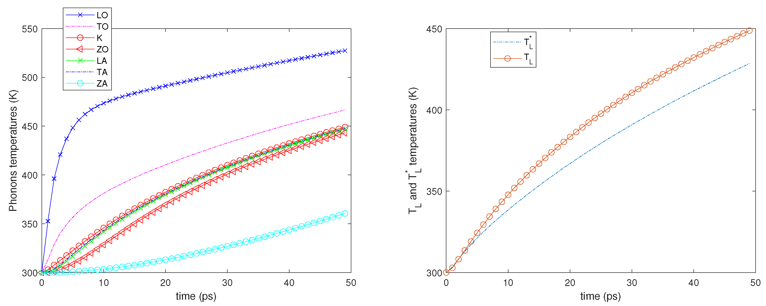
On account of the difficulties with the experimental results, we face the question of analyzing the meaning of the above-mentioned two local lattice temperatures with two numerical experiments. In the first one, coupled electron–phonon simulations are performed, while in the second one, only phonon transport is considered. The hydrodynamic model in [
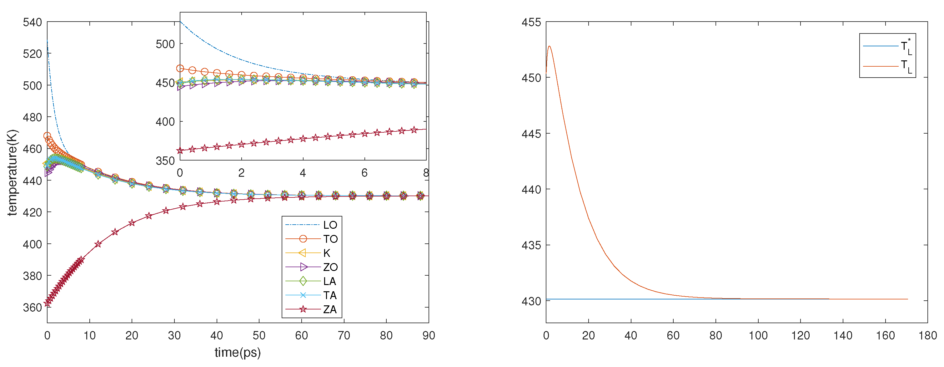
17] is adopted, with a more accurate approximation of the phonon–phonon collision operator. The obtained results, particularly the second set of simulations, strongly indicate that the appropriate definition of the local equilibrium lattice temperature should be that based on the energy Lagrange multipliers, also in accordance with the current non-equilibrium theory [
24,
26]. In fact, in the second numerical experiment, it remains constant, as it should be, when the total energy is conserved at variance with the other local temperature, which, instead, presents an overshoot during the transient before asymptotically tending to the other temperature. Nevertheless, the definition based on the conservation property of the phonon collision operator has also a physical meaning and can be regarded as a measure of how fast the system is trying to approach the equilibrium.
The plan of the paper is the following. In
Section 2, the kinetic model and the definition of the first local temperature are presented. In
Section 3, a macroscopic model and the definition of the second local temperature are introduced. In
Section 4, the results of the numerical simulations are shown and the difference between the two local temperatures is critically highlighted. Eventually, in
Section 5, we furnish the expression for the macroscopic entropy density for the phonon system by which we prove the asymptotic stability of the phonon equilibrium states and theoretically justify the behavior of the phonon temperatures in the second numerical experiment.
2. The Kinetic Model and the Definition of the First Local Temperature
Graphene consists of carbon atoms arranged in a honeycomb hexagonal lattice. The charge transport is essentially due to the electrons, which are located around the
Dirac points,
K and
, which are the vertices of the hexagonal primitive cell of the reciprocal lattice. At the Dirac points, the valence and conduction bands touch each other, which makes graphene a gapless semimetal. Moreover, having the energy bands in an approximately conical shape, electrons behave as massless Dirac fermions [
8]. If high enough, Fermi levels are considered. It is possible to neglect the dynamics of the electrons in the valence bands, being that the latter ones are fully occupied in this case [
27]. Such a situation is similar to n-type doping for traditional semiconductors. As said, around the equivalent Dirac points, the band energy
is approximately linear.
and the group velocity is given by the following:
where
is the electron wave-vector,
is the (constant) Fermi velocity,
ℏ is the reduced Planck constant, and
is the position of the Dirac point
.
In the framework of the semiclassical kinetic theory, relative to the electrons in the conduction band, the charge transport is described by two Boltzmann equations for the
K and
valleys:
where
represents the distribution function of the electrons in the valley
ℓ (
K or
), at position
, time
t, and with wave-vector
. By
and
, we denote the gradients with respect to the position and the wave-vector, respectively;
e is the elementary (positive) charge; and
is the external applied electric field.
The collision term at the right-hand side of (
2) describes the scatterings occurring between electrons and phonons. They can be with longitudinal, transversal, acoustic or optical phonons, which are labeled by LA, TA, LO and TO, respectively. Both the acoustic and the optical phonon scatterings are intra-valley and intra-band. One also has to take into account the electron scattering with
K phonons, which is inter-valley, pushing electrons from a valley to the nearby one. The general form of the collision term is as follows:
where the total transition rate
is given by the sum of the contributions of the several types of scatterings [
17]:
The index
labels the
th phonon mode and
is its angular frequency;
labels the region in the Brillouin zone corresponding to the valley
ℓ. The
’s are the electron–phonon coupling matrix elements, which describe the interaction mechanism of a
th phonon with an electron, going from the state of wave-vector
belonging to the valley
to the state with wave-vector
, belonging to the valley
ℓ. The symbol
denotes the Dirac distribution;
is the phonon distribution for the
-type phonons; and
is the phonon wave-vector belonging to the first Brillouin zone
, measured from
or
K, respectively, for
and
K phonons. In Equation (
3),
, where
, stemming from the momentum conservation. The
K and
valleys can be treated as equivalent; therefore, in the following, we will take into account a unique electron population.
Similarly, the evolution of the phonon populations is determined by the following Boltzmann equations for the phonon distributions as follows:
where
is the acoustic phonon group velocity.
The optical phonon group velocity can be neglected because of the Einstein approximation , which can be used for their dispersion relation, while, regarding the LA and TA phonons, the Debye approximation can be employed: , with the sound speed of the branch ac = LA, TA. Eventually, the dispersion relation of the ZA phonons is approximately quadratic: , with = 0.62 nm/ps.
The phonon collision term splits into two parts as follows:
where the term
is the phonon–electron collision operator, while
represents the phonon–phonon interactions, which are very difficult to treat from a numerical point of view. For this reason, a BGK approximation is commonly used for them [
16]:
which describes the relaxation of each phonon branch toward the equilibrium condition that corresponds to the local equilibrium Bose–Einstein distributions.
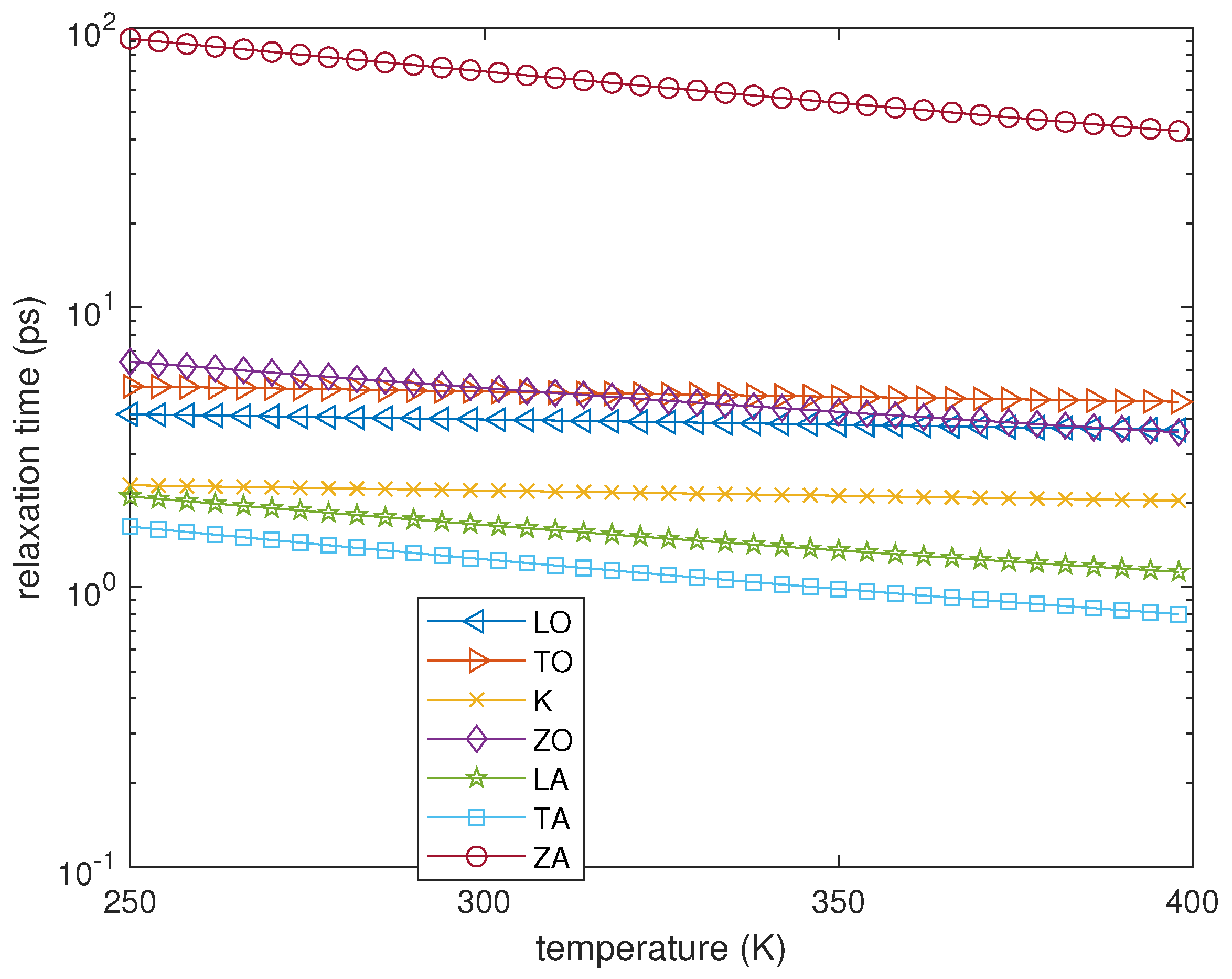
The functions
, which are reported in
Figure 1, are the relaxation times, each of them depending only on the temperature
of the branch under consideration. The temperature
is the same for each phonon population and is defined as follows.
If the phonon distributions
are known, the average phonon energy densities can be calculated as follows:
where
represents the
th phonon density of the states, and the temperature
of each phonon branch is determined from the following condition:
where
varies over the phonon branches.
From the conservation of the total phonon energy, under processes involving only phonons, the following relation has to hold:
where
is calculated by means of (
7) and (
8). The above-written condition allows one to state the following definition of local temperature.
Definition 1. We define as the solution of the non-linear relation (10), which can be obtained numerically; see e.g., [28,29] where this local temperature is called scattered phonon pseudo-temperature. It is possible to prove that (
10) admits a unique solution. For further details, we refer to [
10], where the previous approach was adopted to devise a simulation scheme for the electron–phonon transport in graphene.
3. A Macroscopic Model and the Definition of the Second Local Temperature
Macroscopic models can be derived from the kinetic one [
17,
19,
30] by taking suitable moments of the distribution functions as state variables. Here, we present in some detail only the evolution equations of the phonon variables, and refer the interested reader to [
17] for a complete treatment of the problem.
If one chooses a certain number of moments of the electron and phonon distributions as state variables, the extra fluxes and the production terms, which are present in the corresponding balance equations, are additional unknown quantities, which require constitutive relations in terms of the state variables. By exploiting the maximum entropy principle (MEP), the electron and phonon distributions can be estimated by the so-called maximum entropy distributions
and
,
= LO, TO, ZO, K, LA, TA, ZA, which solve the following maximization problem:
under the constraint that the moments chosen as fundamental variables are known.
is the total entropy of the physical system, which depends on the electron and phonon distribution functions
f and
, and whose expression is reported in [
17].
In particular, for the phonons, the following moments can be chosen:
which respectively represent the energy and momentum densities of the optical phonons and the energy and energy flux densities of the acoustical phonons. Solving the above constrained maximization problem, one obtains the following:
where the
s are the Lagrange multipliers arising from the presence of the constraints.
In order to tackle the problem of the inversion of the constraints, the distribution functions are linearized around their isotropic part, obtaining the following:
By substituting the latter expressions into the constraints (
11) and (12) and by solving them with respect to the Lagrange multipliers, one finds the following:
where
,
is the zeta function,
with
nm being the nearest neighbor distance between the atoms in graphene.
Eventually, using the MEP distribution functions and the relations expressing the Lagrange multipliers as functions of the fundamental variables, it is possible to close the moment equations as follows:
by means of the following closure relations for the production terms
,
, and the acoustical phonon fluxes of energy fluxes
:
where
is the identity matrix, the indices vary over the above-specified phonon branches, and only the productions due to the phonon interactions among themselves are considered.
In the previous section, we introduced a local lattice temperature by the relation (
10), which stems from the properties of the phonon–phonon collision operator. However, the concept of temperature out of equilibrium is a subtle topic and still a matter of debate [
24,
26]. The rationale of the previous definition is that the collision operator
pushes the system, in a characteristic time-related manner to the relaxation times toward a local equilibrium state with a single temperature for all the phonons. However, in statistical mechanics, one of the most reasonable and adopted ways to generalize the concept of temperature in a non-equilibrium state is that of relating it to the Lagrange multipliers associated to the energy constraint.
For the phonon transport in graphene, the approach based on the Lagrange multipliers was followed in [
17] (which the interested reader is referred to for the details) within the application of the MEP (see [
18,
21] for a review of MEP in semiconductors). Let us recall here the main steps.
At equilibrium, the phonon temperatures are related to the corresponding Lagrange multipliers by means of the following:
If we assume that such relations hold, even out of equilibrium, the definition of a second local temperature can be given in terms of the Lagrangian multipliers as follows.
Definition 2. The local temperature of a system of two or more branches of phonons is , where is the common Lagrange multiplier that the occupation numbers of the branches, taken into account, would have if they were in the local thermodynamic equilibrium corresponding to their total energy density, that is, the following:where the sum is extended to the considered branches and the functions are found from expressions (13) and (14). In other words, we require that is such that, by evaluating all the average phonon energy densities with the Lagrange multiplier given by and by summing them up, one obtains the value of the total average energy density.
The two definitions of local temperature are equivalent if, and only if, all the relaxation times are equal, that is, the following:
but this assumption is not compatible with the experimental data as clearly indicated in
Figure 1, where the relaxation times of all the phonon branches are reported [
31]. As a consequence, the two definitions of temperature do not coincide unless all the phonons are in local equilibrium among them, that is, they all have the same local temperature. We notice that
is related only to the energy of the system and does not take into account any scattering mechanism. However, the collision terms are now expressed in terms of the Lagrange multipliers associated to the energies. In fact, the strength of the energy production terms is proportional, according to the relaxation times, to the differences between the energy densities relative to the different Lagrange multipliers and
.
6. Conclusions
Two different definitions of local temperature were compared: one, , based on the properties of the phonon–phonon collision operator, and the other, , based on the energy Lagrange multipliers. Since it is difficult to have a clear meaning of the experimental results, the analysis was based on two numerical experiments represented by simulations of charge and phonon transport in suspended monolayer graphene. The results indicate that the temperature has to be intended as a measure of how fast the phonon system is trying to converge to the local equilibrium, while is the local equilibrium lattice temperature. We have also provided an explicit expression of the phonon entropy density in the homogeneous case.
The case of phonon transport in graphene is particularly challenging because, apart from its own interest due to the increasing importance of thermal effects in nano devices, it has several degrees of freedom—the several branches—and each of them possesses a different temperature. Therefore, one is faced with several important questions of non-equilibrium thermodynamics: the definition of temperature, the interaction among the several degrees of freedom, and the identification of a local temperature.
What was found contributes to the complex and controversial debate about the concept of temperature out of equilibrium. The definition based on the collision operator (Definition 1 of the paper) is employed within a kinetic context but it is little explored in a general framework of non-equilibrium thermodynamics; see the quoted review articles [
2,
3,
4] where it is not explicitly mentioned. However, being that this temperature is related to the phonon–phonon interactions, that is, to the anharmonic interaction terms, we can say that it, in some sense, recalls the configurational temperature [
6,
7].
The definition based on the energy Lagrange multipliers is consistent with the statistical approach and the application of the maximum entropy principle [
20]. Moreover, as shown in the present paper, for each species, it is related to the entropic definition of non-equilibrium temperature, while for the whole system, such an approach leads to a sort of caloric definition of local temperature out of equilibrium.


