
DLSTM-Based Successive Cancellation Flipping Decoder for Short Polar Codes


Abstract
:1. Introduction
- A DLSTM-based SC flipping decoder is proposed. In addition, all frozen bits are clipping in the output layer to enhance accuracy. We construct the flipping set of the first error bit according to the probability of the network output in descending order, and attempt one-bit flipping.
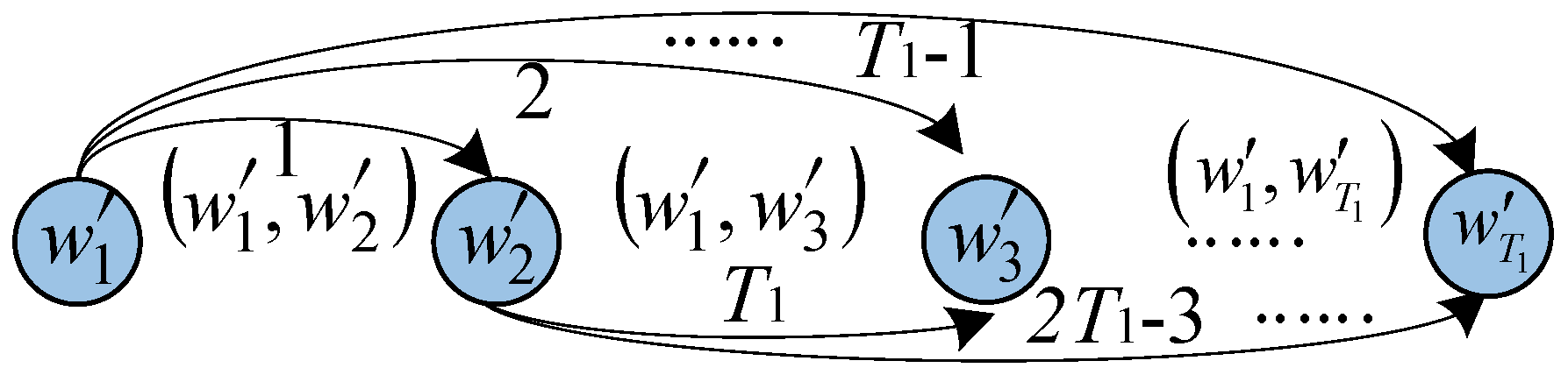
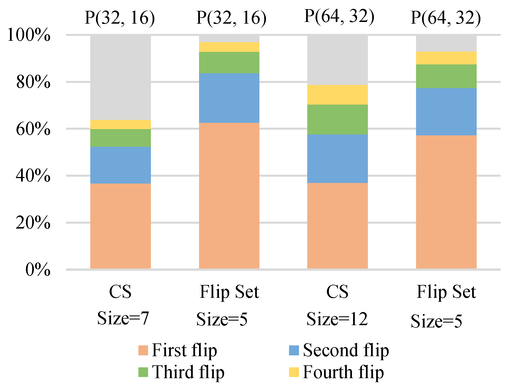
- By exploring the reliability of bit channel, we propose a novel multi-bit flipping scheme for sequences that reach the maximum number of one-bit flipping and still fail the CRC detector. The candidate bits are sorted in ascending order in terms of the reliability, and the unreliable bits are selected in priority to multi-bit flipping.
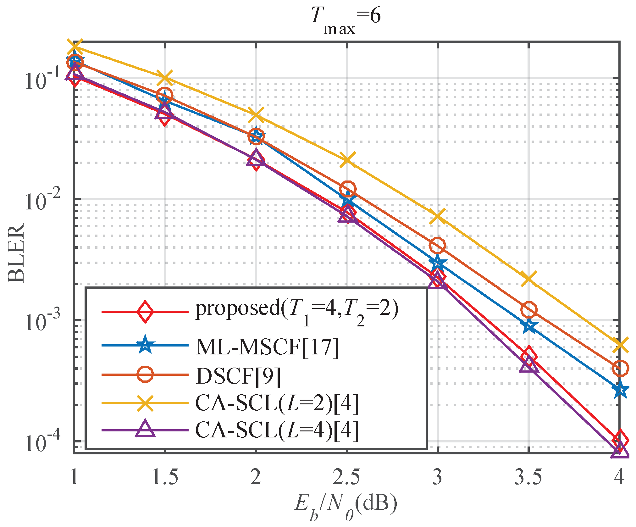
- In order to make the proposed algorithm robust, we design the DLSTM network architecture to be compatible with multiple block lengths. We adopt a padding strategy to maintain data integrity, so that the training is not limited by the block length. A masking method is taken to skip the timestep and eliminate the effect of padded invalid data. Simulation results show that the proposed decoding scheme has better error-correction performance than the ML-MSCF decoding and DSCF decoding for short block lengths. It can approach the performance of CA-SCL (L = 8).
2. Preliminary
2.1. Polar Codes
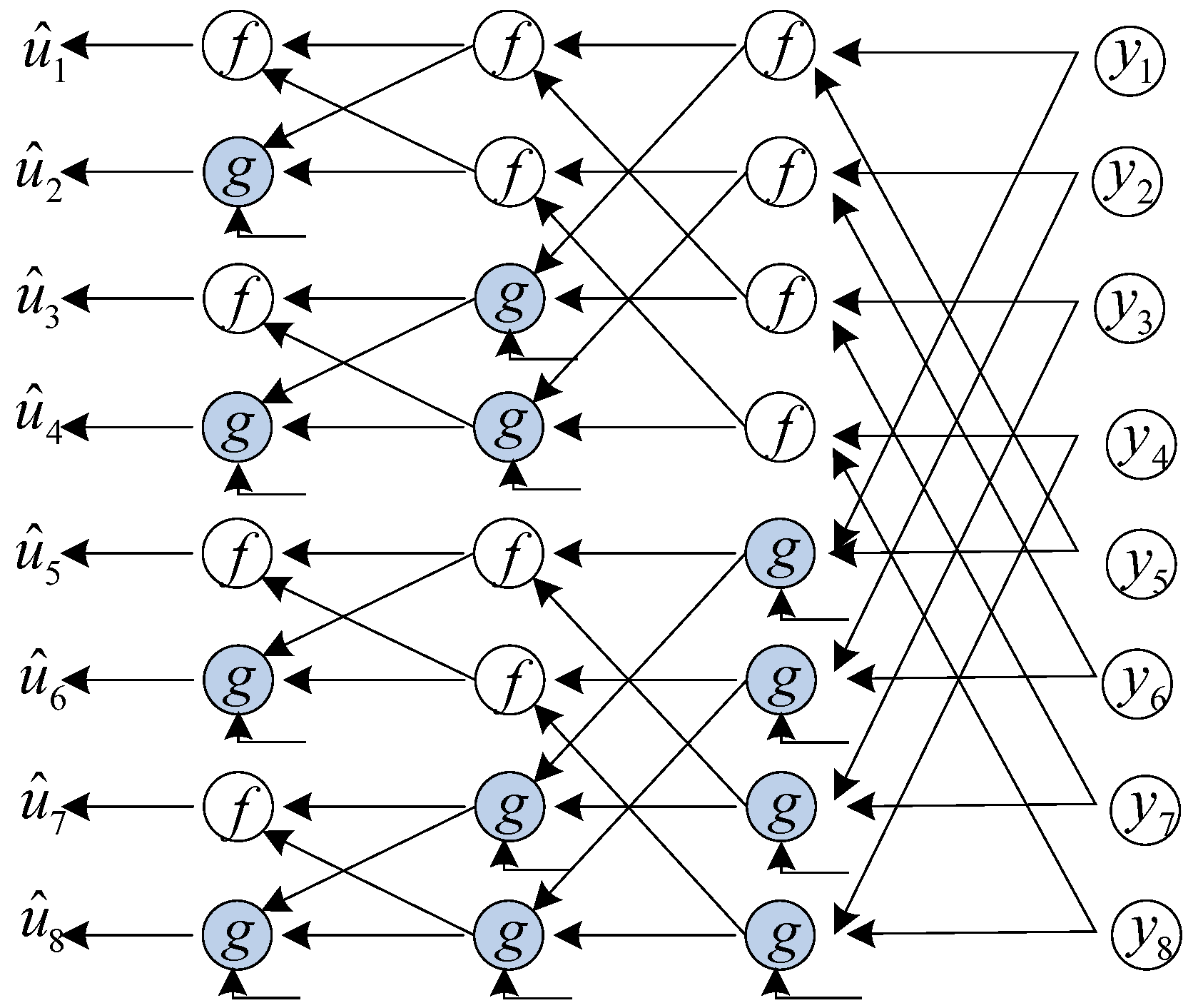
2.2. SC Flipping Decoder
| Algorithm 1 The SC flipping algorithm. |
| Input:, , T Output:
|
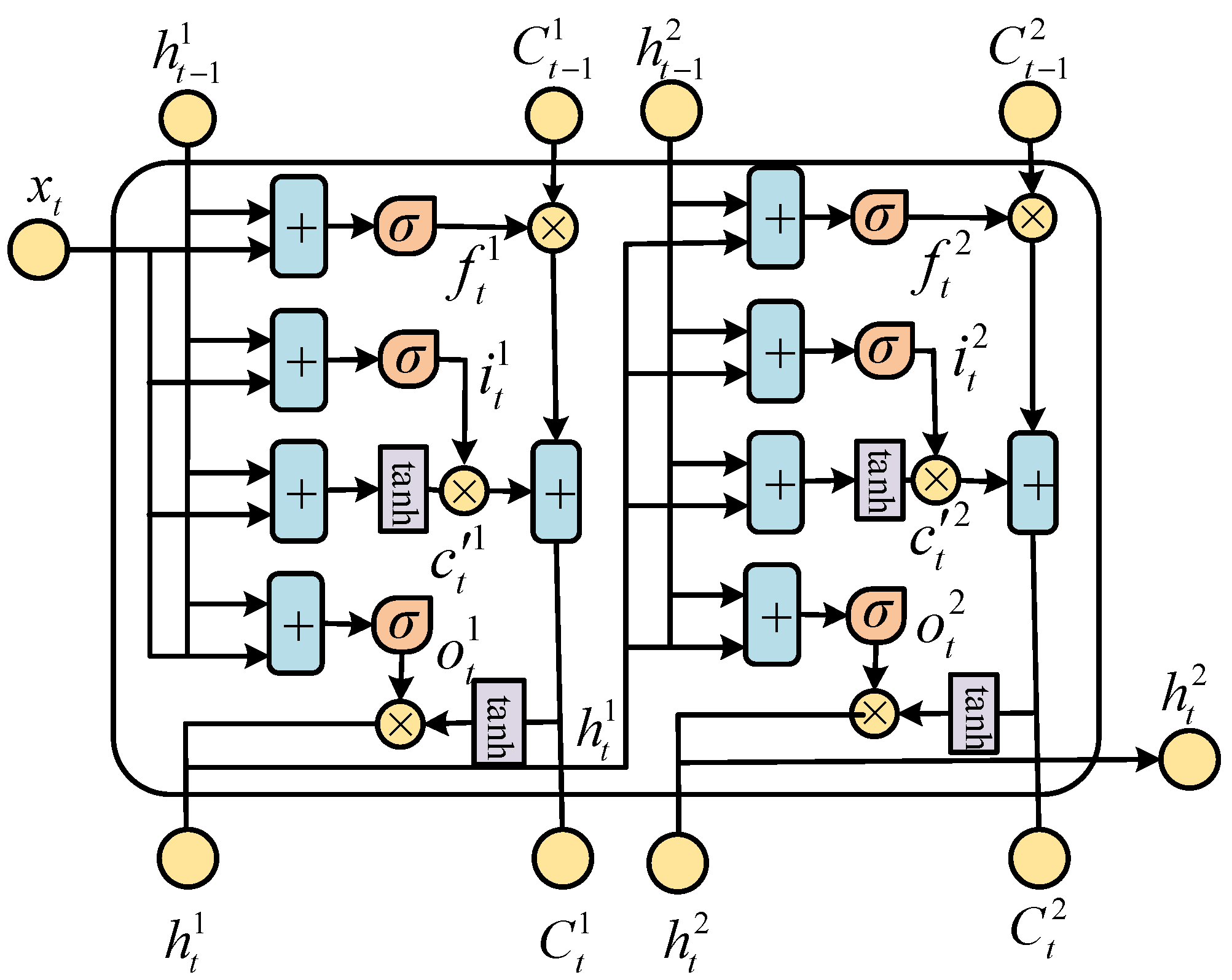
2.3. LSTM Network
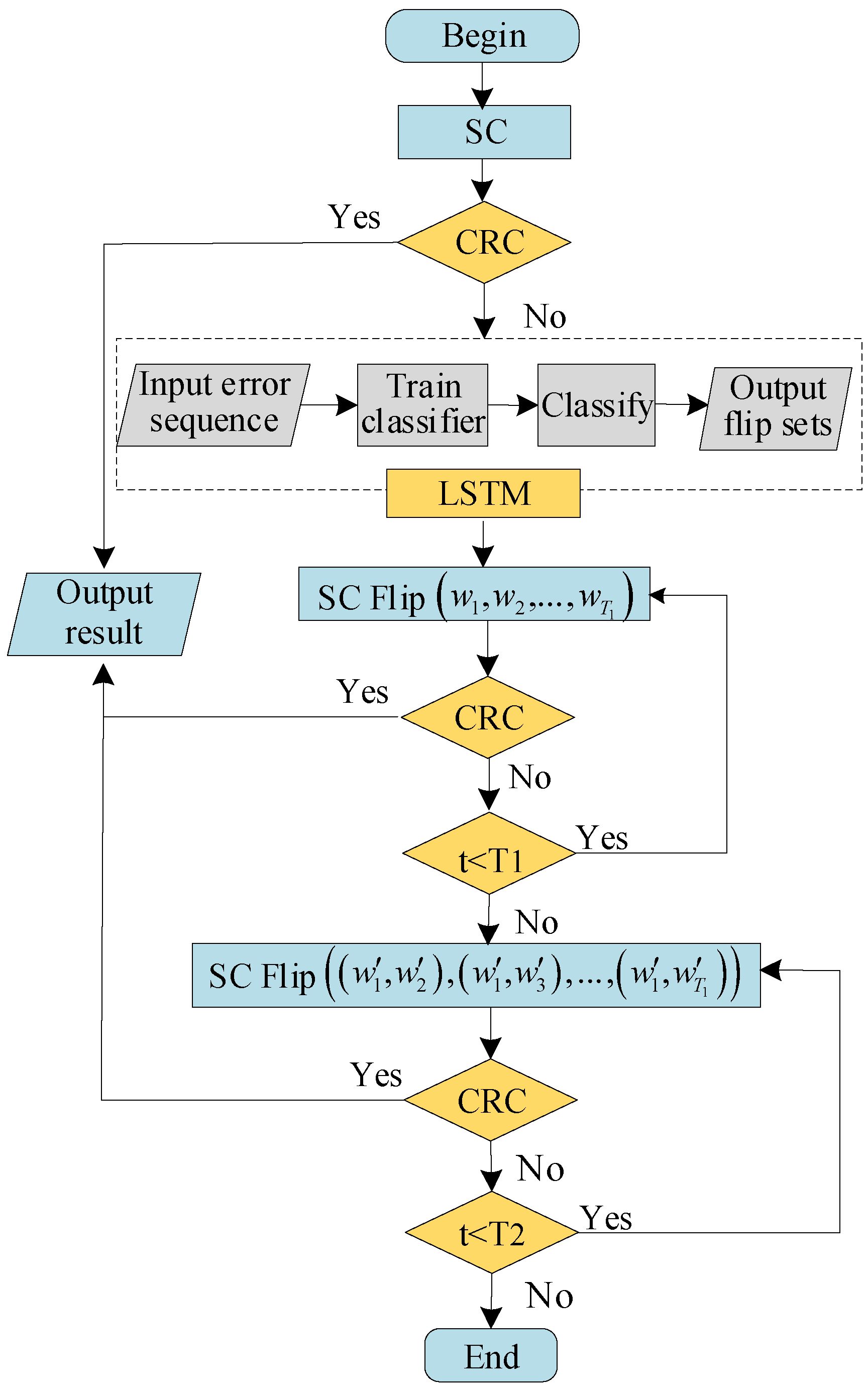
3. The Proposed SC Flipping Algorithm
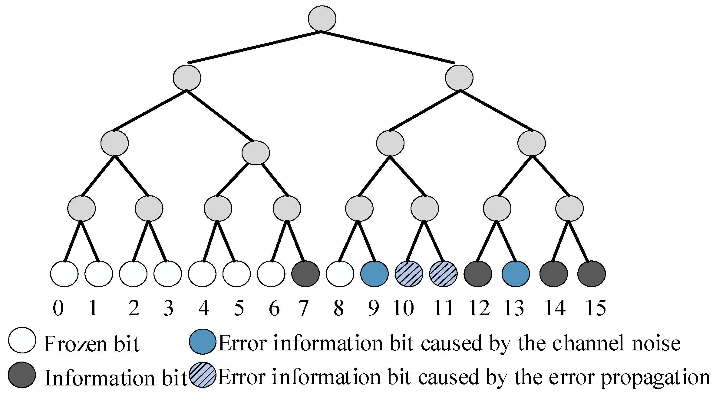
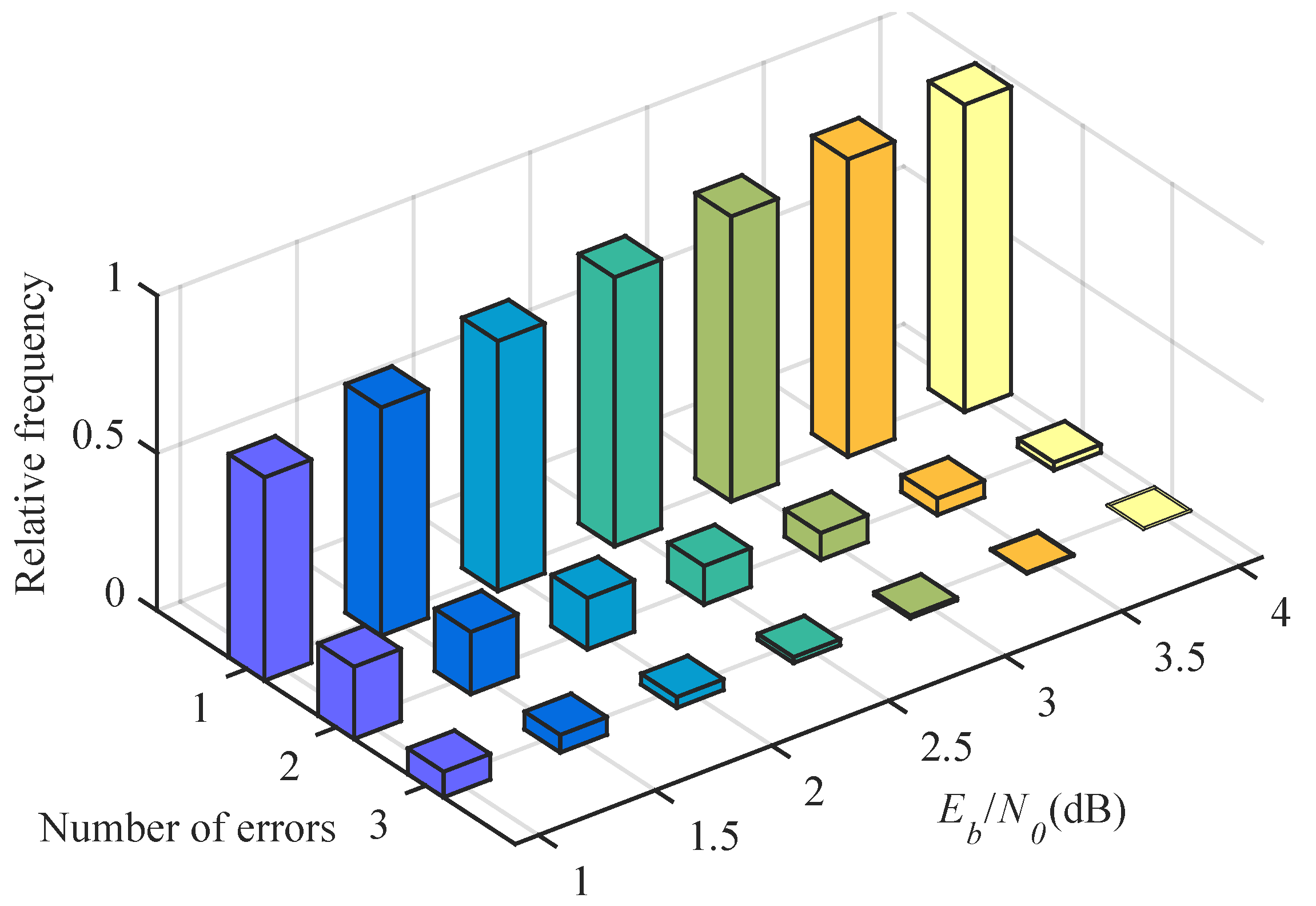
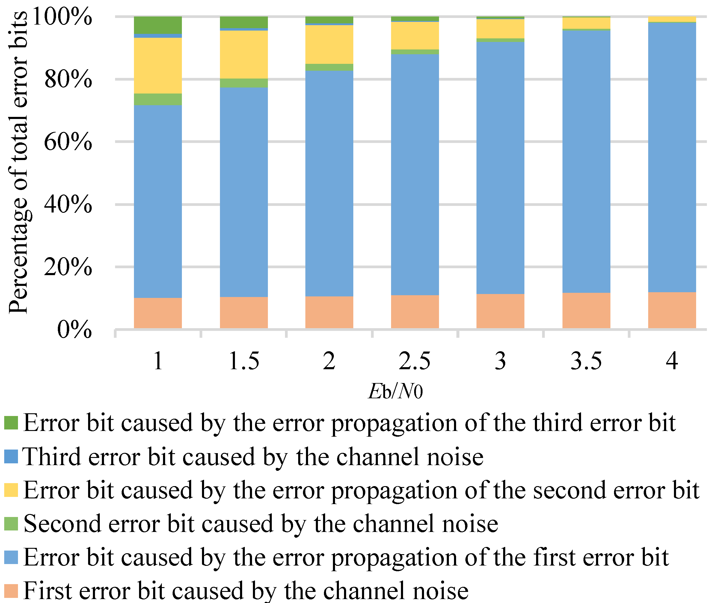
3.1. Analysis of Error Propagation
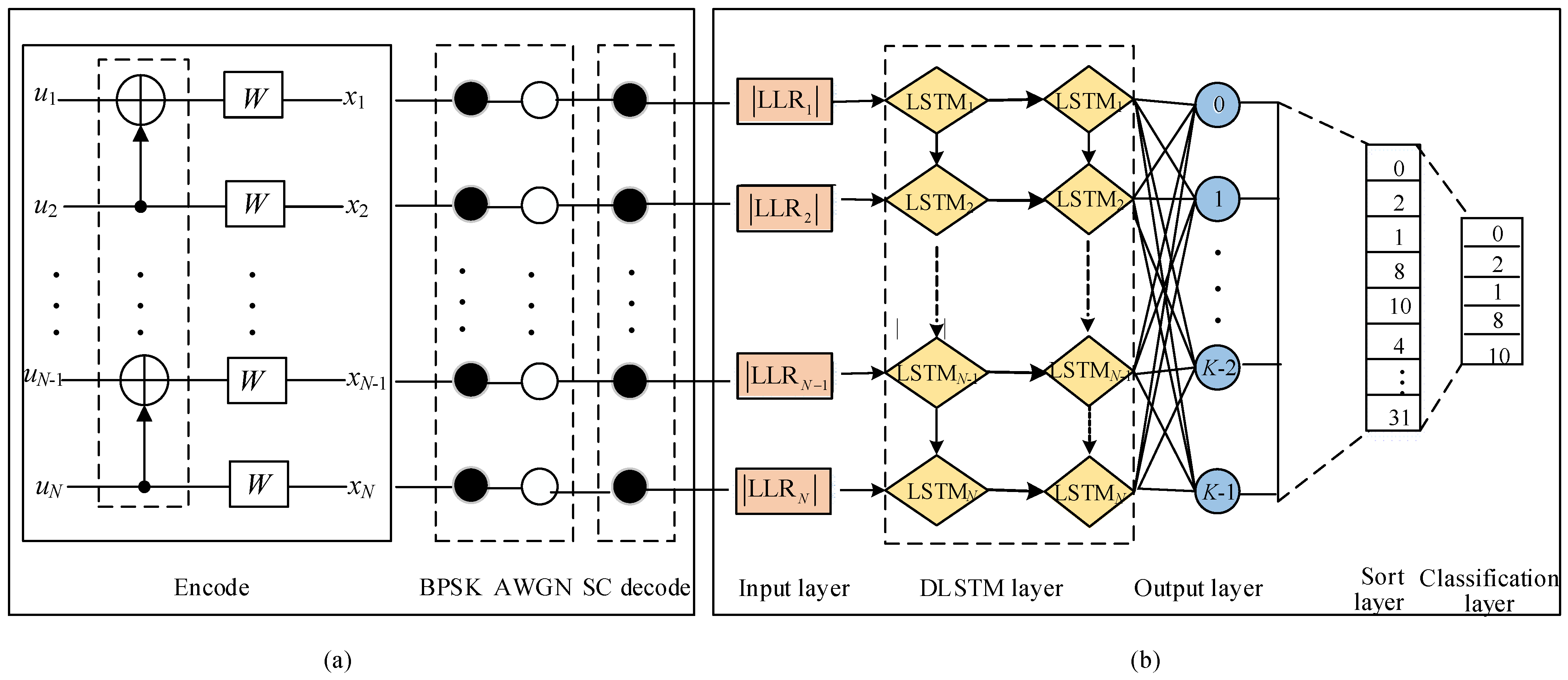
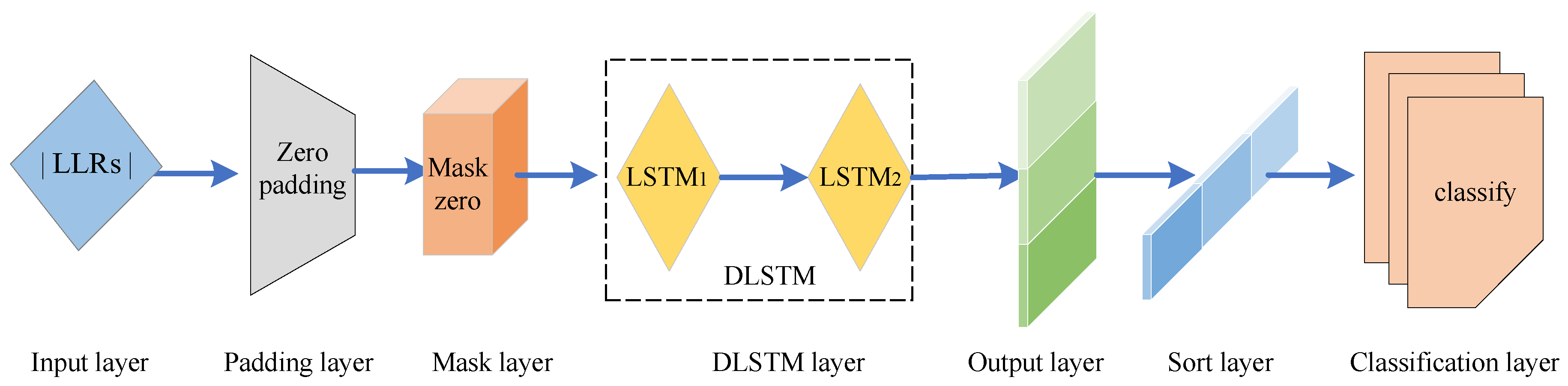
3.2. DLSTM Network Structure
- Input: The absolute value of the LLR sequence (both the information bits and the frozen bits) that fails CRC detector in the SC decoding.
- Output: A K-dimensional vector, the element of which corresponds to the probability of error occurrence for each information bit.
3.3. Training Process of the DLSTM Network
3.4. DLSTM-Based SC Flipping Algorithm
| Algorithm 2 Two-bit flipping algorithm based on the DLSTM. |
| Input:, , , , Output:
|
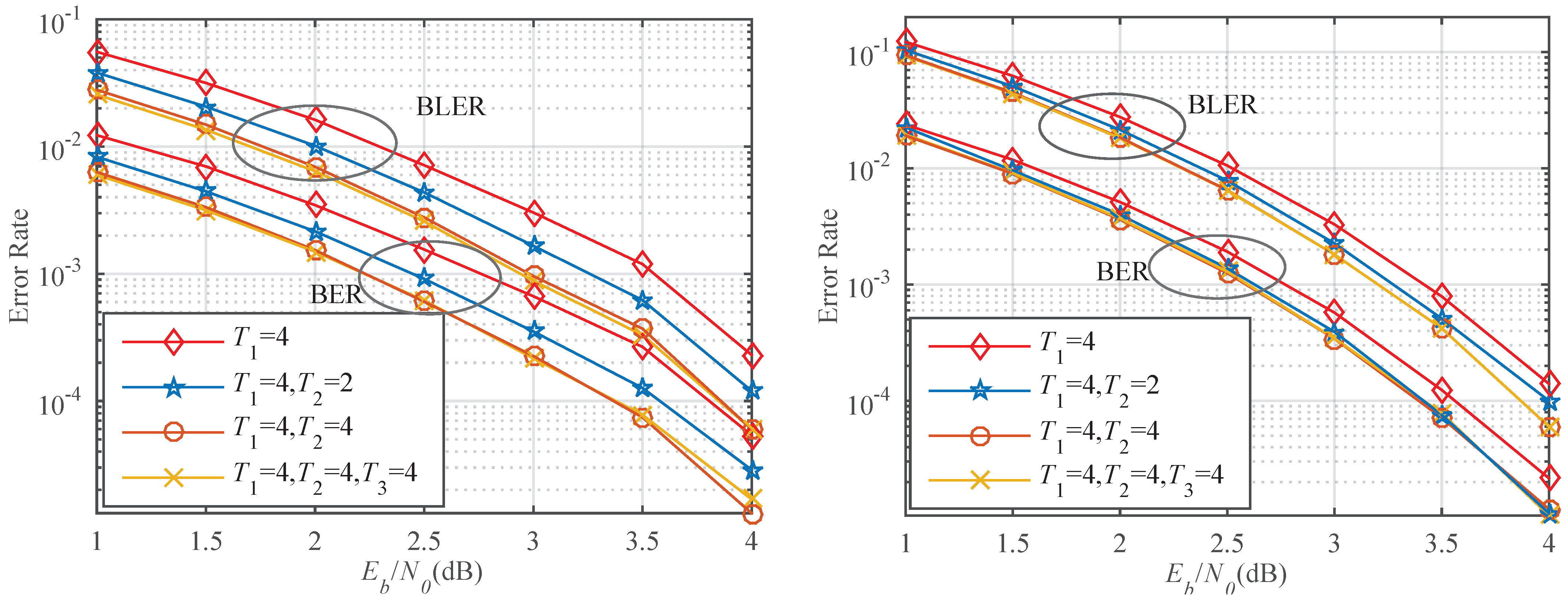
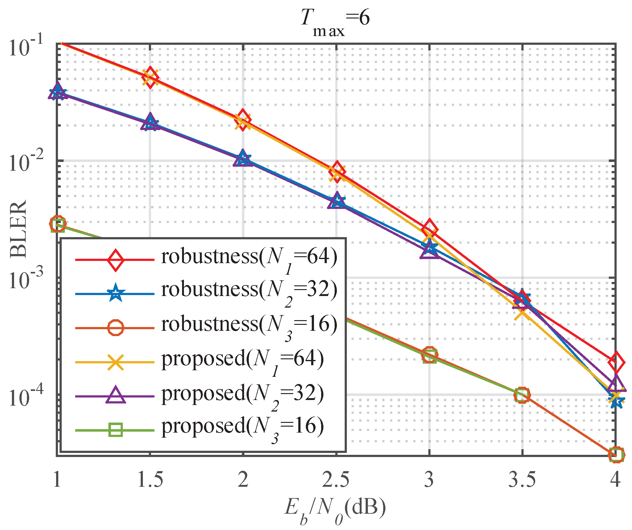
3.5. DLSTM-Based Robustness Mechanism
4. Performance Analysis
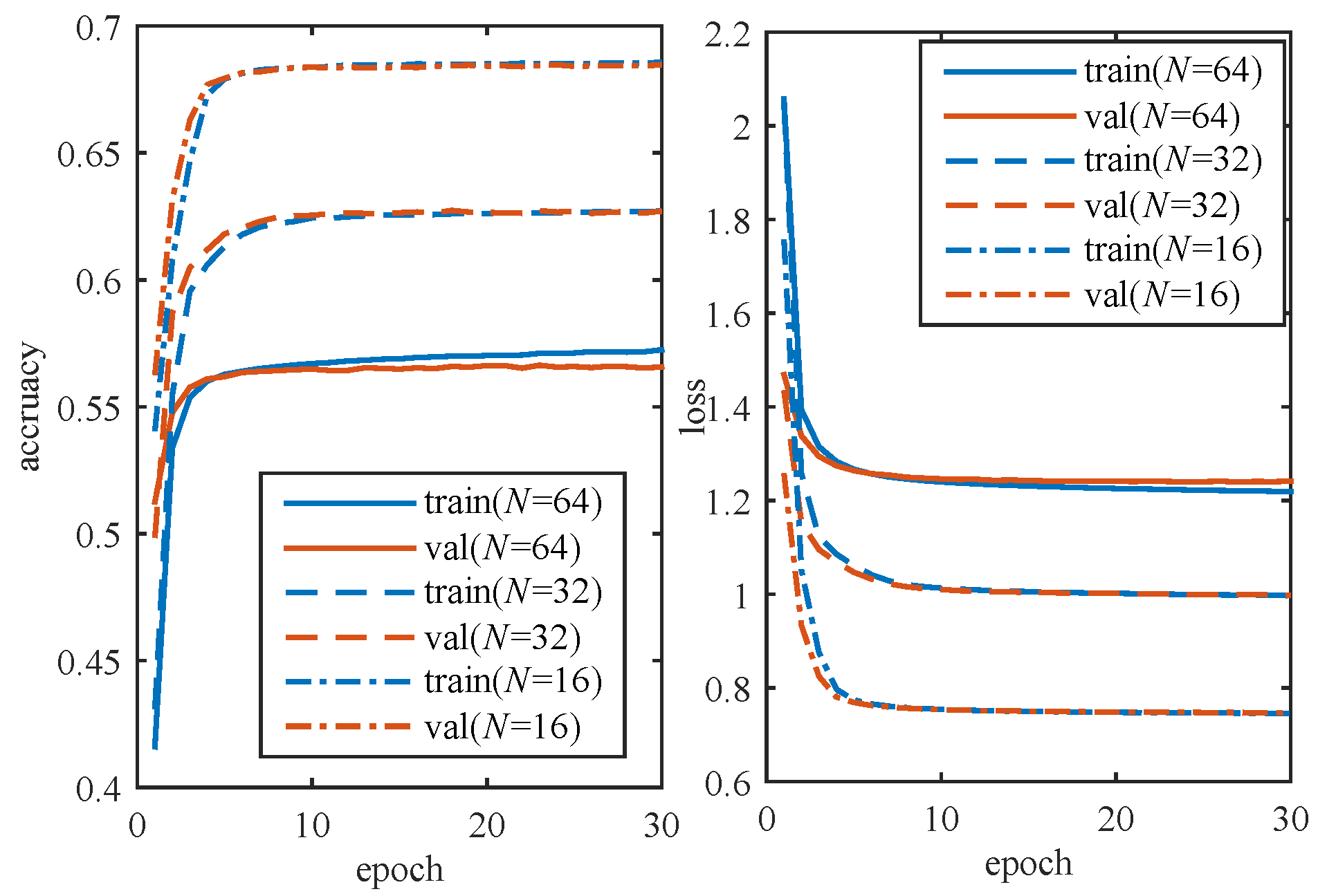
4.1. DLSTM Network Training Results
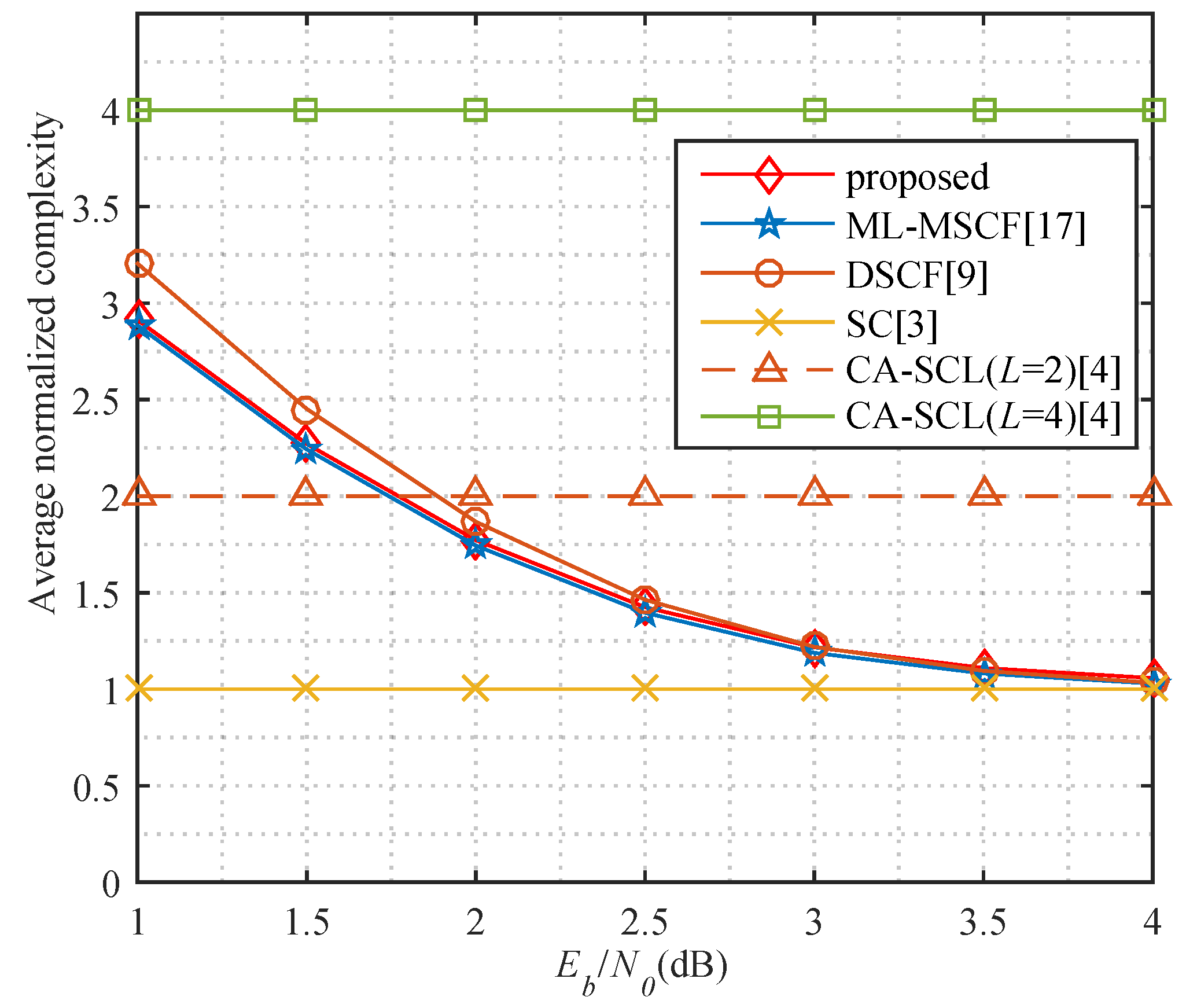
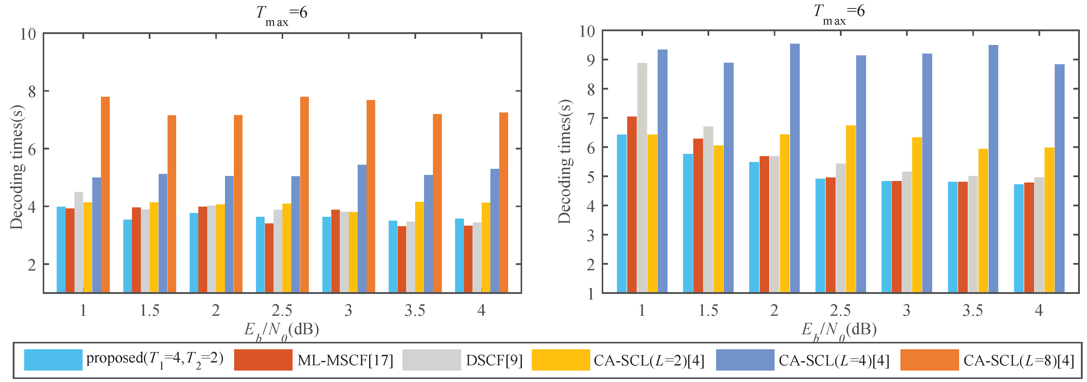
4.2. Decoding Complexity and Latency Analysis
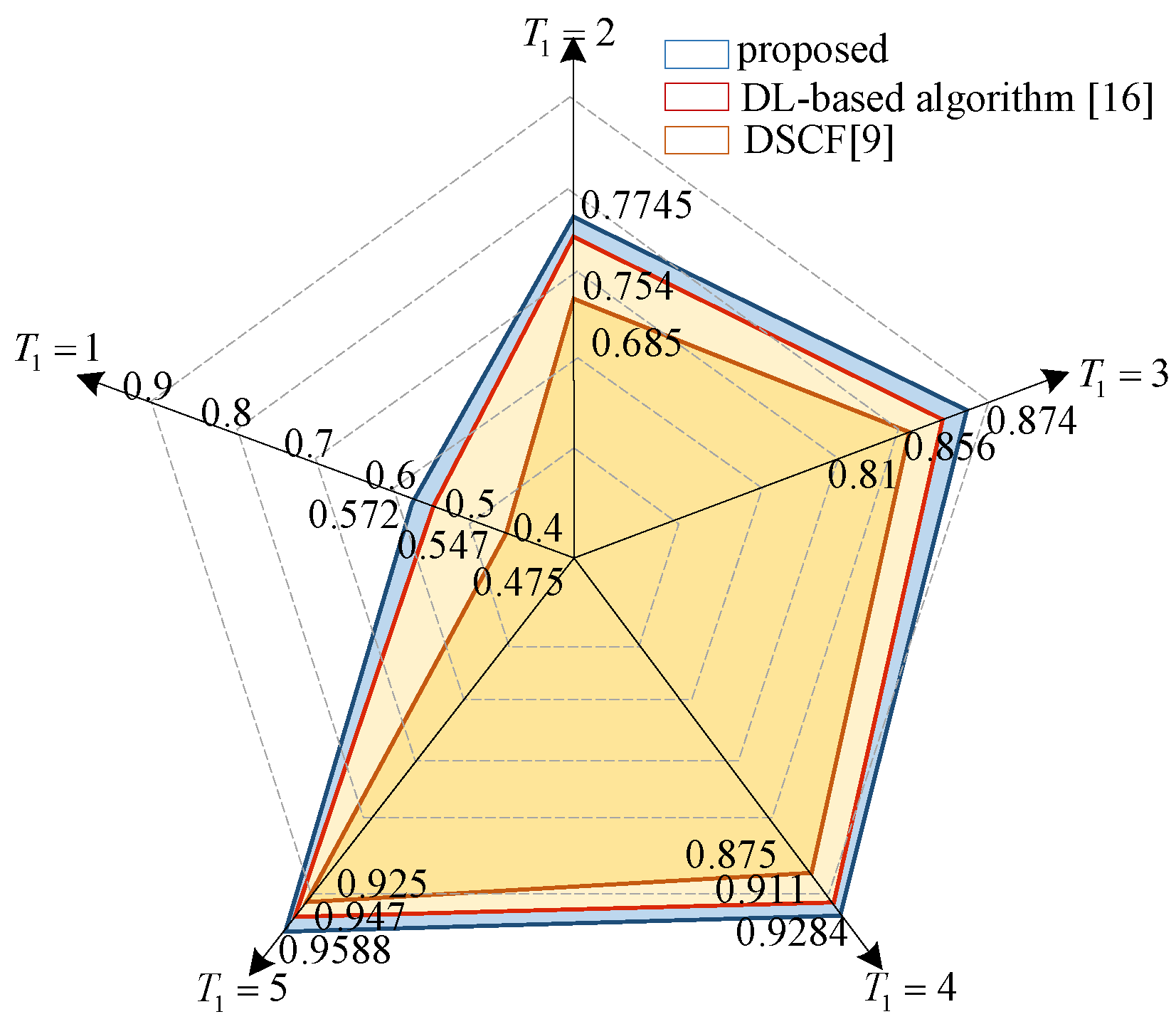
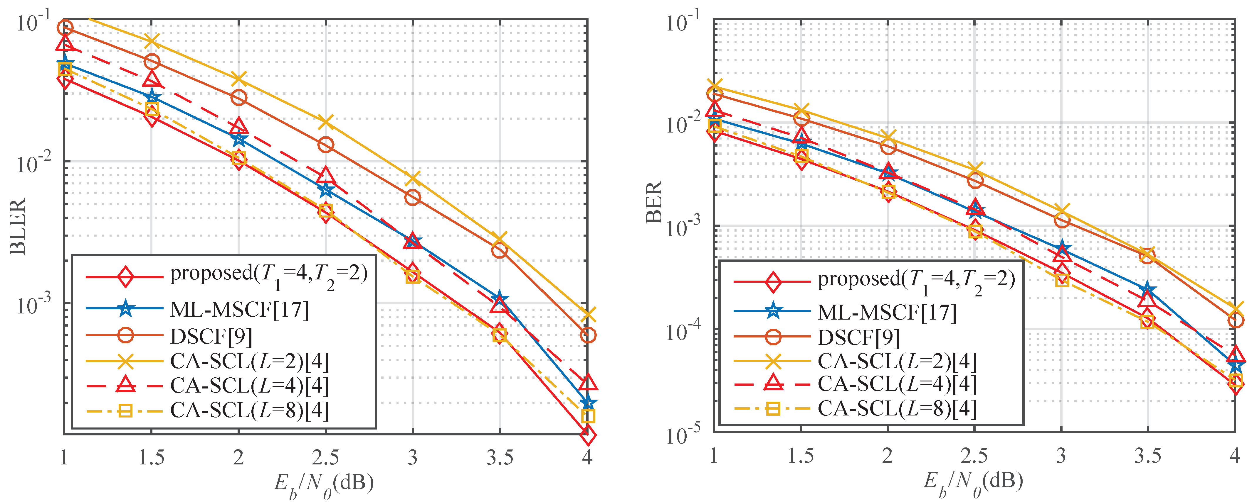
4.3. BER and BLER Analysis
4.4. BLER Analysis of the Algorithm with Robustness Mechanism
5. Conclusions
Author Contributions
Funding
Institutional Review Board Statement
Informed Consent Statement
Data Availability Statement
Conflicts of Interest
Abbreviations
| 5G | Fifth generation |
| SC | Successive cancellation |
| DLSTM | Double long short term memory |
| CRC | Cyclic redundancy check |
| LLR | Log-likelihood ratio |
| CS | Critical set |
| BER | Bit error rate |
| BLER | Block error rate |
| BPSK | Binary phase shift keying |
| AWGN | Additive white Gaussian noise |
References
- Arıkan, E. Channel polarization: A method for constructing capacity-achieving codes. In Proceedings of the 2008 IEEE International Symposium on Information Theory, Toronto, ON, Canada, 6–11 July 2008; pp. 1173–1177. [Google Scholar]
- Final Report of 3GPP TSG RAN WG1 #87 v1.0.0; Reno, USA. November 2016. Available online: https://www.3gpp.org/ftp/tsg_ran/WG1_RL1/TSGR1_87/Report/Final_Minutes_report_RAN1%2387_v100.zip (accessed on 5 January 2021).
- Arıkan, E. Channel Polarization: A method for constructing capacity-achieving codes for symmetric binary-input memoryless channels. IEEE Trans. Inf. Theory 2009, 55, 3051–3073. [Google Scholar] [CrossRef]
- Niu, K.; Chen, K. CRC-aided decoding of polar codes. IEEE Commun. Lett. 2012, 16, 1668–1671. [Google Scholar] [CrossRef]
- Tal, I.; Vardy, A. How to construct polar codes. IEEE Trans. Inf. Theory 2013, 59, 6562–6582. [Google Scholar] [CrossRef] [Green Version]
- Afisiadis, O.; Balatsoukas-Stimming, A.; Burg, A. A low-complexity improved successive cancellation decoder for polar codes. In Proceedings of the 2014 48th Asilomar Conference on Signals, Systems and Computers, Pacific Grove, CA, USA, 2–5 November 2014; pp. 2116–2120. [Google Scholar]
- Chandesris, L.; Savin, V.; Declercq, D. An improved SCFlip decoder for polar codes. In Proceedings of the 2016 IEEE Global Communications Conference (GLOBECOM), Washington, DC, USA, 4–8 December 2016; pp. 1–6. [Google Scholar]
- Zhang, Z.; Qin, K.; Zhang, L.; Chen, G.T. Progressive bit-flipping decoding of polar codes over layered critical sets. In Proceedings of the IEEE Global Communications Conference (GLOBECOM), Singapore, 4–8 December 2017; pp. 4–8. [Google Scholar]
- Chandesris, L.; Savin, V.; Declercq, D. Dynamic-SCFlip decoding of polar codes. IEEE Trans. Commun. 2018, 66, 2333–2345. [Google Scholar] [CrossRef] [Green Version]
- Doan, N.; Ali Hashemi, S.; Gross, W.J. Neural successive cancellation decoding of polar codes. In Proceedings of the 2018 IEEE 19th International Workshop on Signal Processing Advances in Wireless Communications (SPAWC), Kalamata, Greece, 25–28 June 2018; pp. 1–5. [Google Scholar]
- Doan, N.; Hashemi, S.A.; Ercan, F.; Tonnellier, T.; Gross, W.J. Neural dynamic successive cancellation flip decoding of polar codes. In Proceedings of the 2019 IEEE International Workshop on Signal Processing Systems (SiPS), Nanjing, China, 20–23 October 2019; pp. 272–277. [Google Scholar]
- Dhok, A.; Bhole, S. ATRNN: Using seq2seq approach for decoding polar codes. In Proceedings of the 2020 International Conference on COMmunication Systems & NETworkS (COMSNETS), Bengaluru, India, 7–11 January 2020; pp. 662–665. [Google Scholar]
- Qin, Y.; Liu, F. Convolutional neural network-based polar decoding. In Proceedings of the 2019 2nd World Symposium on Communication Engineering (WSCE), Nagoya, Japan, 20–23 December 2019; pp. 189–194. [Google Scholar]
- Wen, C.; Xiong, J.; Gui, J.; Shi, J.; Wang, Y. A novel decoding scheme for polar code using convolutional neural network. In Proceedings of the 2019 IEEE International Symposium on Broadband Multimedia Systems and Broadcasting (BMSB), Jeju, Korea, 5–7 June 2019; pp. 1–5. [Google Scholar]
- Chen, C.; Teng, C.; Wu, A. Low-Complexity LSTM-assisted bit-flipping algorithm for successive cancellation list polar decoder. In Proceedings of the 2020 IEEE International Conference on Acoustics, Speech and Signal Processing (ICASSP), Barcelona, Spain, 4–8 May 2020; pp. 1708–1712. [Google Scholar]
- Wang, X.; Zhang, H. Learning to flip successive cancellation decoding of polar codes with LSTM networks. In Proceedings of the 2019 IEEE 30th Annual International Symposium on Personal, Indoor and Mobile Radio Communications (PIMRC), Istanbul, Turkey, 8–11 September 2019; pp. 1–5. [Google Scholar]
- He, B.; Wu, S.; Deng, Y.; Yin, H.; Jiao, H.; Zhang, Q. A machine learning based multi-flips successive cancellation decoding scheme of polar codes. In Proceedings of the 2020 IEEE 91st Vehicular Technology Conference (VTC2020-Spring), Antwerp, Belgium, 25–28 May 2020; pp. 1–5. [Google Scholar]
- Kasongo, S.M.; Sun, Y. A Deep Long Short-Term Memory based classifier for Wireless Intrusion Detection System. ICT Express 2020. [Google Scholar] [CrossRef]
- Wen, G.; Qin, J.; Fu, X.; Yu, W. DLSTM: Distributed Long Short-Term Memory Neural Networks for the Internet of Things. IEEE Trans. Netw. Sci. Eng. 2021. [Google Scholar] [CrossRef]
- Hochreiter, S.; Schmidhuber, J. Long short-term memory. Neural Comp. 1997, 9, 1735–1780. [Google Scholar] [CrossRef] [PubMed]
- Yang, H.; Ma, J.H. Research on method of regularization parameter solution. Comput Meas. Control 2017, 25, 226–229. [Google Scholar]
- Kingma, D.P.; Ba, J.L. Adam: A method for stochastic optimization. In Proceedings of the ICLR 2015, San Diego, CA, USA, 7–9 May 2015. [Google Scholar]
- Zhang, Z.; Niu, K.; Dong, C. Multi-bit-flipping decoding of polar codes based on medium-level bit-channels sets. In Proceedings of the IEEE Wireless Communications and Networking Conference (WCNC), Marrakesh, Morocco, 15–18 April 2019; pp. 1–6. [Google Scholar]
- Shantharama, P.; Thyagaturu, A.S.; Reisslein, M. Hardware-Accelerated Platforms and Infrastructures for Network Functions: A Survey of Enabling Technologies and Research Studies. IEEE Access 2020, 8, 132021–132085. [Google Scholar] [CrossRef]


| Index | 0 | 1 | 2 | 3 | 4 | 5 | 6 | 7 | 8 | 9 | 10 | 11 | 12 | 13 | 14 | 15 |
|---|---|---|---|---|---|---|---|---|---|---|---|---|---|---|---|---|
| Location | 0 | 0 | 0 | 0 | 0 | 0 | 0 | 1 | 0 | 1 | 1 | 1 | 1 | 1 | 1 | 1 |
| Index of information bit | 0 | 1 | 2 | 3 | 4 | 5 | 6 | 7 |
| Name | Parameter |
|---|---|
| Polar codes | (64,32) |
| Frame number | 2,000,000 |
| Rate R | 1/2 |
| CRC generator polynomial | |
| Batch size | 1000 |
| Number of epoch | 30 |
| Regularization L2 | 0.008 |
| DLSTM | 66,048 |
| Dense | 2080 |
| Optimizer | Adam |
| Polar Codes | Layer | Accuracy | Total Param | |||
|---|---|---|---|---|---|---|
| 2 | 57.2% | 77.45% | 87.4% | 92.84% | 68,128 | |
| 3 | 57.12% | 77.32% | 87.43% | 92.94% | 101,152 | |
| 2 | 68.63% | 91.8% | 98.48% | 99.86% | 4360 | |
| 3 | 68.46% | 91.81% | 98.44% | 99.85% | 6472 | |
| Algorithm | Gain (dB) | Reduce Latency | |
|---|---|---|---|
| proposed | 3.25 | - | - |
| ML-MSCF [17] | 3.53 | 0.28 | −5.77% |
| DSCF [9] | 3.74 | 0.49 | −1.16% |
| CA-SCL (L = 2) [4] | 3.91 | 0.66 | 15.73% |
| CA-SCL (L = 4) [4] | 3.44 | 0.19 | 31.22% |
| CA-SCL (L = 8) [4] | 3.23 | −0.02 | 51.46% |
Publisher’s Note: MDPI stays neutral with regard to jurisdictional claims in published maps and institutional affiliations. |
© 2021 by the authors. Licensee MDPI, Basel, Switzerland. This article is an open access article distributed under the terms and conditions of the Creative Commons Attribution (CC BY) license (https://creativecommons.org/licenses/by/4.0/).
Share and Cite
Cui, J.; Kong, W.; Zhang, X.; Chen, D.; Zeng, Q. DLSTM-Based Successive Cancellation Flipping Decoder for Short Polar Codes. Entropy 2021, 23, 863. https://doi.org/10.3390/e23070863
Cui J, Kong W, Zhang X, Chen D, Zeng Q. DLSTM-Based Successive Cancellation Flipping Decoder for Short Polar Codes. Entropy. 2021; 23(7):863. https://doi.org/10.3390/e23070863
Chicago/Turabian StyleCui, Jianming, Wenxiu Kong, Xiaojun Zhang, Da Chen, and Qingtian Zeng. 2021. "DLSTM-Based Successive Cancellation Flipping Decoder for Short Polar Codes" Entropy 23, no. 7: 863. https://doi.org/10.3390/e23070863
APA StyleCui, J., Kong, W., Zhang, X., Chen, D., & Zeng, Q. (2021). DLSTM-Based Successive Cancellation Flipping Decoder for Short Polar Codes. Entropy, 23(7), 863. https://doi.org/10.3390/e23070863