2.1. The 2-D Modified Hilbert Curve
The original 2-D Hilbert curve connects a square array of the size of
. We denote it as the
order Hilbert curve. Hilbert curves of orders
,
, and
are respectively shown in
Figure 1a–c. There is an important property of the Hilbert curve. As can be seen from
Figure 1a–c, the starting and the ending points (green and red points in the graphs) are always on one side of the
square. Since the starting and the ending points are at the ends of one side of the Hilbert curve square, a Hilbert curve of any order
can easily be represented by a square with labeled starting and ending points like
Figure 1d, when the internal structure does not need to be shown.
Figure 1.
2-D Hilbert curve properties. (a–c) are, respectively, the 1st order, the 2nd order, and the 3rd order Hilbert curves. (d) A simple notation to represent the order 2-D Hilbert curve. (e) Construction of the order Hilbert curve from the order Hilbert curve. (f) Reduction of points on the height for the order Hilbert curve. (g) Increasing of points on the height for the order Hilbert curve.
Now, we can show that an
order Hilbert curve can be easily constructed from four
order Hilbert curves. First, replace the 4 points in the 1
st order Hilbert curve in
Figure 1a with four
order Hilbert curves whose starting and ending points are arranged as indicated in
Figure 1e; then, connect the ending points and starting points of the
Hilbert curves orderly as indicated in
Figure 1e, and the
order Hilbert curve is constructed. With the 1
st order Hilbert curve provided by
Figure 1a and the method of constructing the
order Hilbert curve from the
Hilbert curve, we can construct the Hilbert curve of any order by mathematical induction.
Now, our task is to construct a scanning route that is close to the Hilbert curve for a 2-D array of size , where W and H are the element numbers along the vertical and horizontal direction, respectively.
The basic idea is to divide the
rectangle array into
small square arrays of the size
, and
. For example, a
rectangle array can be divided into three
square arrays with
and
. Apparently, within each square, an
order Hilbert curve can be easily constructed as shown in
Figure 2a. By appropriately arranging the directions of each Hilbert curve, the 3 Hilbert curves are connected to form the desired route, as shown in
Figure 2b.
To form a route close to the Hilbert curve, there are two requirements. First, the largest
needs to be selected in order, i.e., select the largest
first, then the largest
, …, etc. Without this restriction, the constructed curves may deviate from the Hilbert curve significantly. As an extreme example, for the
points in
Figure 2, one can simply choose
, i.e., use the 96 points as 96 small square arrays. In this case, there are too many possible routes. Most of them are not close to the Hilbert curve at all, for example, the raster scan. Secondly, the ending point of the Hilbert curve in the
square must be adjacent to the starting point of the Hilbert curve of the
square, like the example shown in
Figure 2b. For design convenience, the first requirement may not be satisfied strictly sometimes. However, the second requirement must be satisfied.
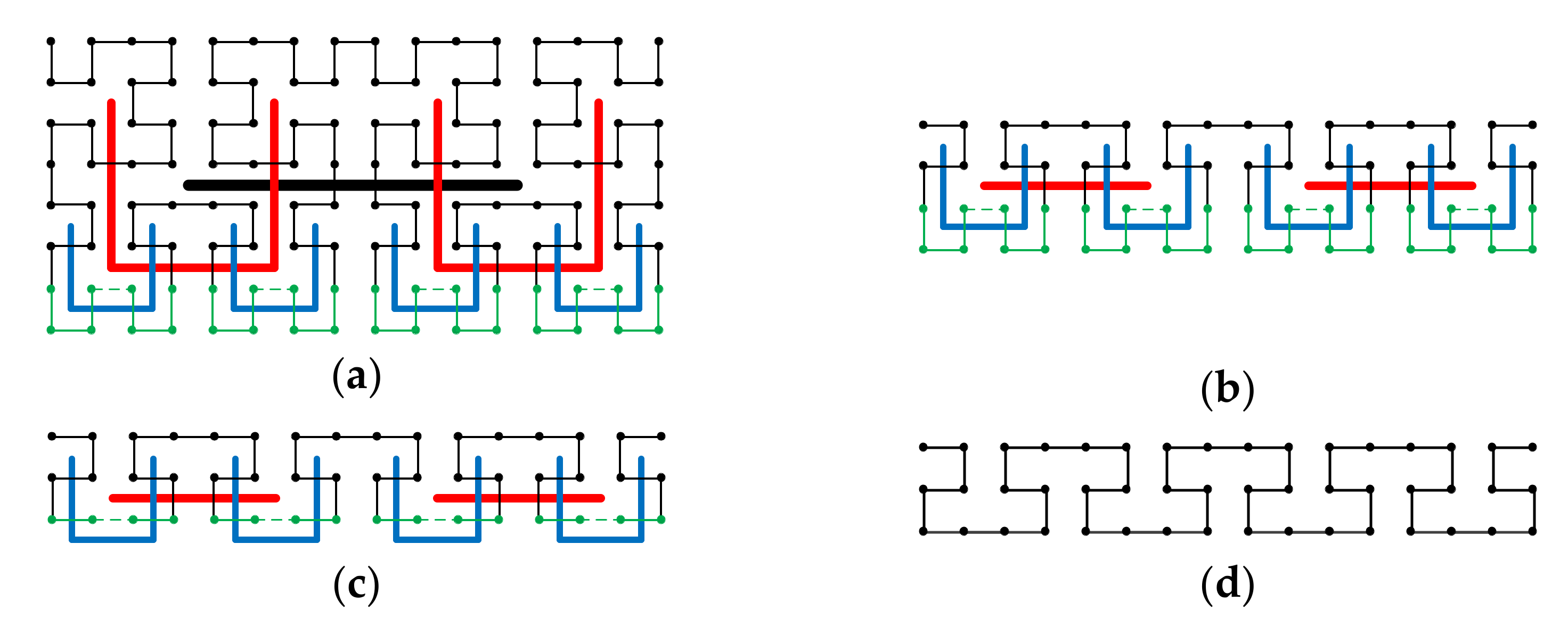
Figure 2.
Construction of the 2-D modified Hilbert curve for the array size 12 × 8. (a) Three Hilbert curves are constructed for the 3 divided sub-square arrays. (b) By selecting appropriate directions for each of the 3 Hilbert curves and connecting the 3 Hilbert curves, the modified 2-D Hilbert curve is constructed.
Figure 3.
Illustration of the 2-D Modified Hilbert curve construction procedures on a rectangle array, where .
Figure 3.
Illustration of the 2-D Modified Hilbert curve construction procedures on a rectangle array, where .
Based on the above observations, the procedures of our design method are provided as follows (note, the method is not unique). Without loss of generality, we consider rectangle arrays with :
Find integer such that and .
Construct a modified Hilbert curve within the sub-rectangle S
1 of size
. S
1 is a special rectangle with the width being
. The starting and the ending points of S
1 need to be at the ends of the S
1’s top width, as indicated in
Figure 3. The construction details for this step is provided shortly. (Note, we use “width” and “height” to represent the number of elements in the two orthogonal directions of a rectangle array throughout the paper. They are not the geometric lengths. Do not get confused with the illustrating diagrams used in the paper.)
Once the modified Hilbert curve for the rectangle array S
1 is constructed, the construction of the remaining rectangle array S
2 goes back to step (1) with the starting and the ending points indicated in
Figure 3. However, the array size of S
2 is less than half of the original
rectangle.
By iterating steps 1 to 3, the subsequent remaining S2’s become smaller and smaller very quickly, with speed faster than , where is the iteration number. The iteration stops when the remaining S2 is of size , and the construction is complete. Note, a size of can always be achieved because the smallest can be 1.
Note, when iterating the three steps 1 to 3, if for S
2, the height
is larger than
like the situation shown in
Figure 3, then
plays the role of the width
for the new iteration on S
2 because we assumed the initial condition of
for each iteration. In this case, the design route changes direction because it is always along the width direction, see
Figure 3. If for S
2 the height
is still smaller than
, the iteration continues along the same design route direction. In the following example, we show a specific design to provide a more intuitive understanding of the procedures.
Suppose we want to design a modified 2-D Hilbert curve for a practical size of and , which is the subband size from the subband decomposition on a image, the standard HDTV size. Following the design procedures:
Iteration 1:
, and sub-rectangle arrays S
1 and S
2 for the 1st iteration are:
,
, as shown in
Figure 4a.
Iteration 2: Because
, the 135 side of
needs to be the width for the 2nd iteration. Then, for the second iteration on the
array,
, the starting (green) point and the ending (red) point are aligned vertically, changing the design route direction, see
Figure 4b. The resulting sub-rectangle arrays S
1 and S
2 for the 2nd iteration are
,
, as shown in
Figure 4b.
Iteration 3: Because
, the 112 side of
needs to be the width in the 3
rd iteration. Then, for the 3
rd iteration on the
array,
, and the starting (green) point and the ending (red) point are aligned horizontally, changing the design route direction again, see
Figure 4c. The resulting sub-rectangles S
1 and S
2 for the 3
rd iteration are:
,
, see
Figure 4c. Note,
in
Figure 4c.
Iteration 4: Because
, the 48 side of
is still the width for the 4
th iteration. Thus, for the 4
th iteration on
,
, the starting (green) point and the ending (red) point are still aligned horizontally, with no design route direction change. The resulting sub-rectangles S
1 and S
2 for the 4
th iteration are:
,
, see
Figure 4c. Note,
in
Figure 4c.
Iteration 5: Similar to Iteration 4, no change of the design route direction is needed. However, the width for the 5
th iteration is
. By selecting
,
, and
, the design completes as indicated in
Figure 4c.
Now we go back to provide the details of step 2 of the design procedures. In other words, we need to design a modified Hilbert curve for a rectangle with the width being and the height being . There are three possible situations, (A) , (B) , and (C) . Condition (C) is trivial, where the sub-rectangle is a square, and the construction is simply the original Hilbert curve.
Condition (A) :
We start from the
order Hilbert curve, whose height is
. Thus, we need to reduce the height by
. Recall that an integer
can be converted into its binary format
, i.e.,
can be decomposed as
where the
’s are either 0 or 1. Decomposing
using (1), we can perform a reduction of
step by step, with each step achieving a reduction of
points. For example, suppose
. Then, from (1), we have
, i.e.,
,
,
, and
. Thus, we need to reduce 8 points, 4 points, and 1 point on
to achieve the total reduction of
points.
To perform a reduction of
points, first, a reduction of
points on the
order Hilbert curve is straightforward. By inspection, it can be seen that the top two sub-squares in
Figure 1e can be removed, leading to
Figure 1f. Then, a reduction of
points on the
order Hilbert curve is achieved.
Figure 4.
The example of designing the 2-D modified Hilbert curve for the 240 × 135 array: (a) the 1st iteration, (b) the 2nd iteration, and (c) the 3rd, 4th, and the 5th iteration.
Figure 4.
The example of designing the 2-D modified Hilbert curve for the 240 × 135 array: (a) the 1st iteration, (b) the 2nd iteration, and (c) the 3rd, 4th, and the 5th iteration.
Next, we observe the following property: For an opening-toward-top Hilbert curve of any order, the bottom sub-Hilbert curves always have the same opening-toward-top orientation. As an example, in
Figure 5a, a 4
th order opening-toward-top Hilbert curve is plotted. The 4
th order Hilbert curve can be represented using the structure of
Figure 5b, i.e., the main structure is an opening-toward-top 1
st order Hilbert curve with 4 sub-curves, which are four 3
rd order Hilbert curves denoted by four small shaded squares. As just described above, the removal of the top two sub-squares, or, equivalently, a reduction of 8 points in
in this case, can be easily achieved. Now, it is important to observe from
Figure 5b that the bottom two shaded squares, i.e., the bottom two 3
rd order sub-Hilbert curves, are also opening-toward-top Hilbert curves. When the original 4
th order Hilbert curve is represented using the structure of
Figure 5c, for each of the bottom two opening-toward-up 3rd order sub-Hilbert curves, the removal of the top two sub-squares, or equivalently a reduction of 4 points on
in this case, can be achieved. Similarly, it can be seen from
Figure 5a,d that reductions of 2 points and 1 point on
can be achieved.
Figure 6 shows a specific example of how the 4
th order Hilbert curve is reduced by
. In
Figure 5a, the original 4
th order
Hilbert curve is shown. Reductions on
by 8, 4, and 1 in each step are respectively shown in
Figure 6a–c. After all the sub-reductions are completed, the total reduction of
is achieved in
Figure 6d.
Figure 5.
(a) The 4th order 2-D Hilbert curve; The 4th order 2-D Hilbert curve represented using (b) four 3rd order sub-curves; (c) sixteen 2nd order sub-curves; and (d) sixty-four 1st order sub-curves.
Figure 5.
(a) The 4th order 2-D Hilbert curve; The 4th order 2-D Hilbert curve represented using (b) four 3rd order sub-curves; (c) sixteen 2nd order sub-curves; and (d) sixty-four 1st order sub-curves.
Condition (B) :
We need to increase the height by
. Note, since
,
, i.e.,
. Thus, similar to condition (A),
is decomposed by (1), and we can increase
by
points in each step because the increase in height by
points on the
order Hilbert curve can be achieved using the modification from
Figure 1e–g.
With the height of the order Hilbert curve reduced or increased to , procedure 2 of the iterative design method described earlier is performed. The modified 2-D Hilbert curve on a rectangle array using the iterative design procedures is completed.
To provide more intuitions, the 2-D modified Hilbert curves of sizes
,
, and
, constructed using the proposed method, are shown in
Figure 7. In addition, the MATLAB codes implementing the proposed method are available in [
19]. As can be easily checked, the algorithm runs reasonably fast, and the results can be obtained instantly.
2.2. The 3-D Modified Hilbert Curve
In [
15], the binary run-length-based symbol grouping entropy coding method is used in video compression. For the 3-D transform video compression algorithm introduced in [
15], conventional motion compensation is not used in order to improve the computational complexity. Instead, a 4-band SCWP transform [
20] is performed along the time dimension. In other words, the first step of the video compression algorithm is a 3-D transform. Thus, the transformed coefficients are 3-D subband arrays.
In entropy coding of the quantized 3-D subband coefficient arrays, the 3-D Hilbert curve scan was used to maximally keep the correlations in the 3-D subband into the 1-D scanned array. Because the original 3-D Hilbert curves are for cubes of side length
, in [
15], the
test videos were cropped to a size of
for testing. Apparently, to accommodate an arbitrary rectangle video size, the original 3-D Hilbert curve needs to be modified. Below, we extend the modification method introduced in
Section 2.1 for 2-D arrays to 3-D conditions. The 3-D arrays are of size
, where
and
are the width and height of the cuboid array,
is the third dimension denoting the depth here, which corresponds to the time dimension of the input video.
The depth
of the 3-D decomposed subband is determined by the parameter “group of pictures” (GOP), which is normally selected to be the powers of 2. As a result, the depths
are also the powers of 2, i.e.,
For example, the GOP used in [
15] was 32, which leads to the depths
of the 3-D subbands being 8, 4, 2, or 1 (for details, please refer to [
15]). Furthermore, compared with
and
,
is normally much smaller in our case.
We begin from the original 3-D Hilbert curve. Again, we denote a 3-D Hilbert curve of size
, the
order 3-D Hilbert curve.
Figure 8a,b, respectively, show the 1
st order and the 2
nd order 3-D Hilbert curve. Similar to the 2-D situation, the starting and the ending points of any order 3-D Hilbert curves are at the two ends of one side of the cube. Therefore, as shown in
Figure 8c, when the internal structure is not needed, a 3-D Hilbert curve of any order
can be represented by a cube with the starting and ending points labeled. With this simple and intuitive representation, the construction of the
order 3-D Hilbert curve from the
order 3-D Hilbert curve can be easily demonstrated by
Figure 8d. By mathematical induction, given (1) the 1
st order 3-D Hilbert curve and (2) the method of constructing the
order 3-D Hilbert curve from the
order 3-D Hilbert curve, the 3-D Hilbert curve of any order can be constructed.
Without loss of generality, assume
. As mentioned in our application,
is the powers of 2 and is normally much smaller than
and
. In other words, the modified 3-D Hilbert curve is of size
, and
is much smaller than
and
. Exploiting these features, the extension to 3-D from 2-D can borrow the 2-D construction procedures introduced in
Section 2.1 as follows.
First, consider the situation where
and
are multiples of
, i.e., the cuboid of size
, where
,
,
and
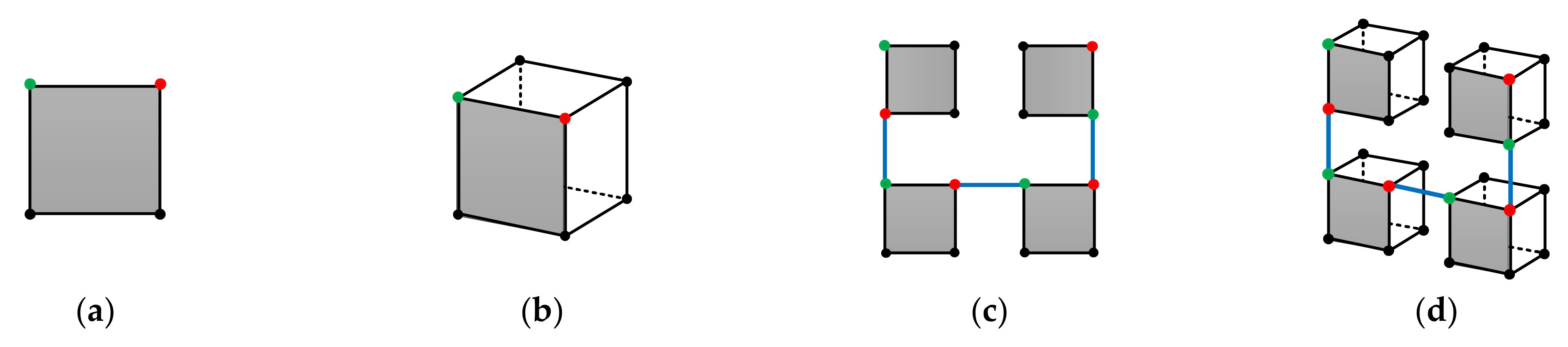
are integers. In this case, we can directly extend the 2-D construction method to 3-D construction. To see that, the
order original 2-D Hilbert curve is compared with the
order original 3-D Hilbert curve in
Figure 9a,b. Because the
cube is the smallest construction block for the 3-D curve and the
square is the smallest construction block for the 2-D curve, the 3-D construction of size
can directly borrow the 2-D construction structure of size
.
Figure 9c,d intuitively show the 2-D to 3-D extension by comparing the 2-D Hilbert curve of size
with the modified 3-D Hilbert curve of size
.
Next, we consider the situation where
and
are not multiples of
, but
. In this case, we can still borrow the 2-D construction structure, i.e., use the 2-D iterative route similar to
Figure 3 and
Figure 4c for the height-width (
-
surface of the 3-D cuboid. This is similar to what we performed in
Figure 9c,d, where
and
are multiples of
. The difference is that, in this case,
is not a multiple of
. In this case, we need to consider the non-zero terms in
that are smaller than
, i.e., the
terms. The
terms are multiples of
, which is the situation previously considered. The
terms in
, however, need to be handled on the 3-D cubes at the bottom. For example, if in
Figure 9d we want to construct a modified 3-D Hilbert curve of size
instead of
, then the bottom cubes in
Figure 9d need to be reduced by
points to achieve
.
Therefore, we need to consider adding or reducing
points on the
cube, where
. This is not difficult. (1) Similar to the 2-D situation, observe in
Figure 10a that the bottom 4 sub-cubes (sub-Hilbert curves) are of the same opening-toward-top orientation as its original 3-D Hilbert curve because they all have the starting and ending points at the top surface of the cube. (2) For the 3-D Hilbert curve of size
, indicated in
Figure 10a, reducing and increasing
points on
can be achieved by
Figure 10b,c respectively. Combining (1) and (2) above, reducing or increasing
points on
can be achieved on a 3-D Hilbert curve of size
.
Figure 8.
3-D Hilbert curve properties. (a,b) are respectively the 1st order and the 2nd order 3-D Hilbert curves. (c) A simple notation to represent the order 3-D Hilbert curve. (d) Construction of the order Hilbert curve from the order Hilbert curve.
Figure 8.
3-D Hilbert curve properties. (a,b) are respectively the 1st order and the 2nd order 3-D Hilbert curves. (c) A simple notation to represent the order 3-D Hilbert curve. (d) Construction of the order Hilbert curve from the order Hilbert curve.
Figure 9.
Extension of the 2-D construction to 3-D construction for size , where and are integers. (a) The smallest construction block for 2-D, the square. (b) The smallest construction block for 3-D, the . cube. (c) The size 2-D Hilbert curve, constructed from the 2-D smallest construction block. (d) The size 3-D Hilbert curve, constructed from the 3-D smallest construction block borrowing the 2-D construction structure of (c).
Figure 10.
Point increasing and reducing operations on the order 3-D Hilbert curve. (a) The order 3-D Hilbert curve. (b) The points are reduced on . (c) The points are increased on . (d) The situation where points need to be increased in a different direction.
Figure 10.
Point increasing and reducing operations on the order 3-D Hilbert curve. (a) The order 3-D Hilbert curve. (b) The points are reduced on . (c) The points are increased on . (d) The situation where points need to be increased in a different direction.
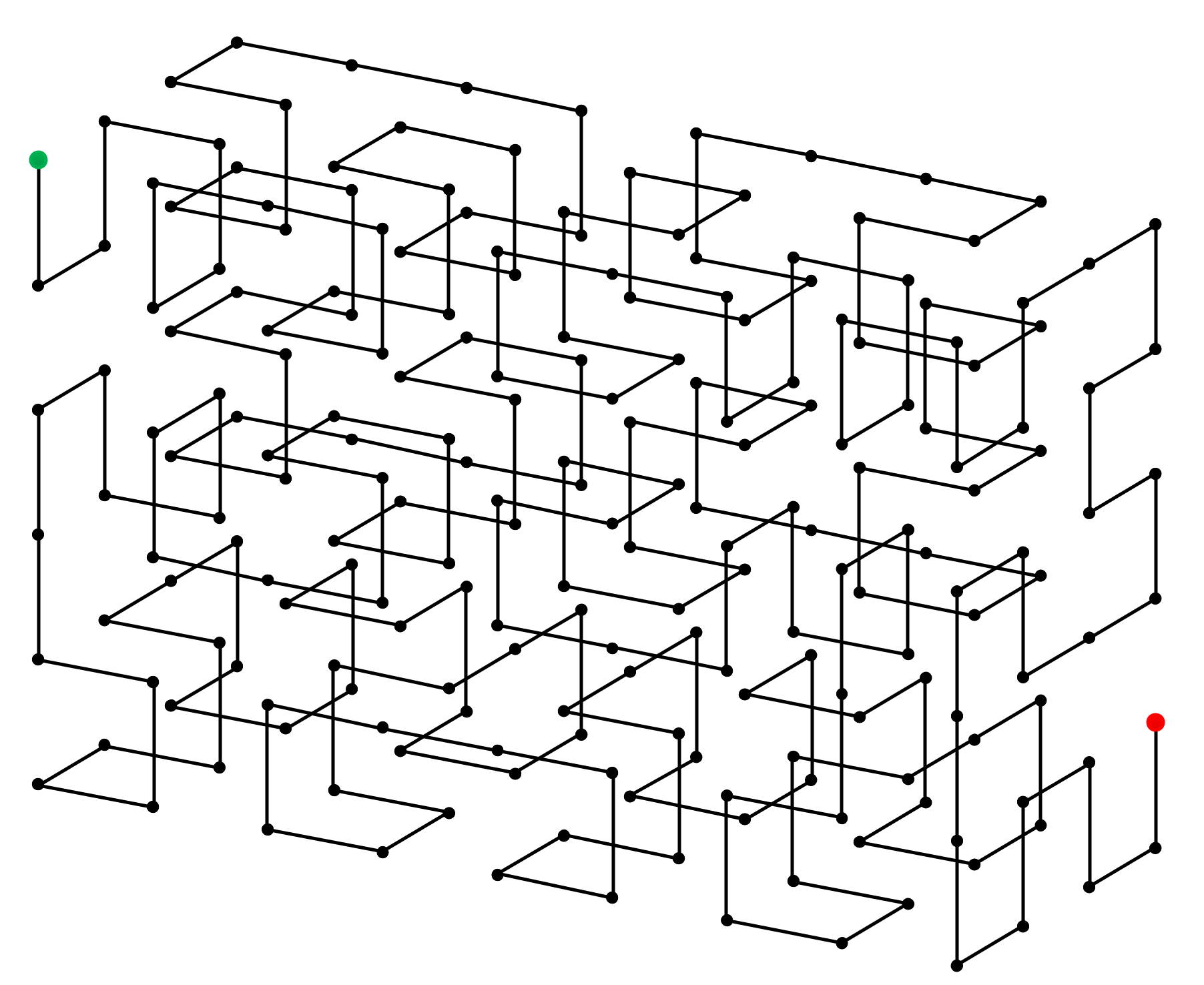
Figure 11.
The modified 3-D Hilbert curve of size , constructed using the proposed method.
Figure 11.
The modified 3-D Hilbert curve of size , constructed using the proposed method.
Finally, during the 3-D construction described above, for the height-width (
-
surface of the 3-D cuboid, we can exploit the 2-D iterative route similar to
Figure 3 and
Figure 4c as long as
is satisfied for the remaining S
2’s in the
-
surface. For example, we can realize the modified 3-D Hilbert curve for the size of
following exactly the 2-D route shown in
Figure 4c, which was used for constructing the
2-D modified Hilbert curve. Nevertheless, a construction may end up with a residue S
2 on the
-
surface, whose height and width are both smaller than
. For example, using the above method to construct the modified 3-D Hilbert curve of the size
, we end up with a residue cuboid of size
. Then, the 2-D
Figure 3 iterative procedure cannot proceed for the
-
surface anymore. We have to consider the situation of constructing a modified 3-D Hilbert curve of the size
with
.
However, in the 3-D transform video application,
is very small. As mentioned above, in [
15], the maximum
even if the GOP used is 32. When
, the maximum residue cuboid is only 7 × 7 × 8, which is very small. For such tiny residue cuboids, using some other routes, such as the raster scan, would not lead to any noticeable effect on the final video compression results. On the other hand, the design for the situation of
is complex, and thus, for the application of coding the 3-D transformed coefficients in video compression, we can just use a simple scan route for the residue cuboids with
. We implemented in MATLAB such 3-D extension with small
residue cuboid connected using the raster scan, which is available at [
19].
Figure 11 shows a modified 3-D Hilbert curve of size
(i.e.,
produced by MATLAB codes.
We will not lengthily go into the design on the condition . For completeness, we only briefly describe that the design is possible using similar ideas we have used up to now. Note, there can be some other methods to handle the situation because the design method is not unique.
For the situation, first, consider the situation where either or is a power of 2. Without loss of generality, assume . Observe that the sizes , , …, etc., i.e., all the 6 permutations, are the same for our curve construction task. In order to exploit our previously developed construction techniques, we need to change the roles of , , and . Because is the longest side, we need to use as the width. Since , use as the depth. Then, the construction finishes nicely in one step.
For the more difficult situation, where both
and
are not powers of 2, decompose the shortest side
into a sum of
using equation (1):
, where
(
corresponds to the most significant bit, i.e.,
). Then, the construction on the
cuboid is immediately achieved as described above. To increase the thickness from
to
, the point-increasing operation needs to be along the direction as illustrated in
Figure 10d. For the 4 length-increased sub-cubes at the back in
Figure 10d, the bottom 2 sub-cubes can use the point-increasing operation we already used, i.e., the one from
Figure 10a to
Figure 10c, but the top 2 sub-cubes need to use a different point-increasing structure, which is skipped here. We may also need to perform multiple point-increasing operations and then perform a point-decreasing operation to achieve the desired value
, and the operations need to be performed individually for the sub-cubes at the back of the
cuboid. The sizes of the sub-cubes can be different depending upon the
value. As a result, the implementation is complex. We will not go into the details further since currently, there is no immediate application.


