
The Multi-Focus-Image-Fusion Method Based on Convolutional Neural Network and Sparse Representation


Abstract
:1. Introduction
2. Related Works and Discussion
2.1. Sparse Representation
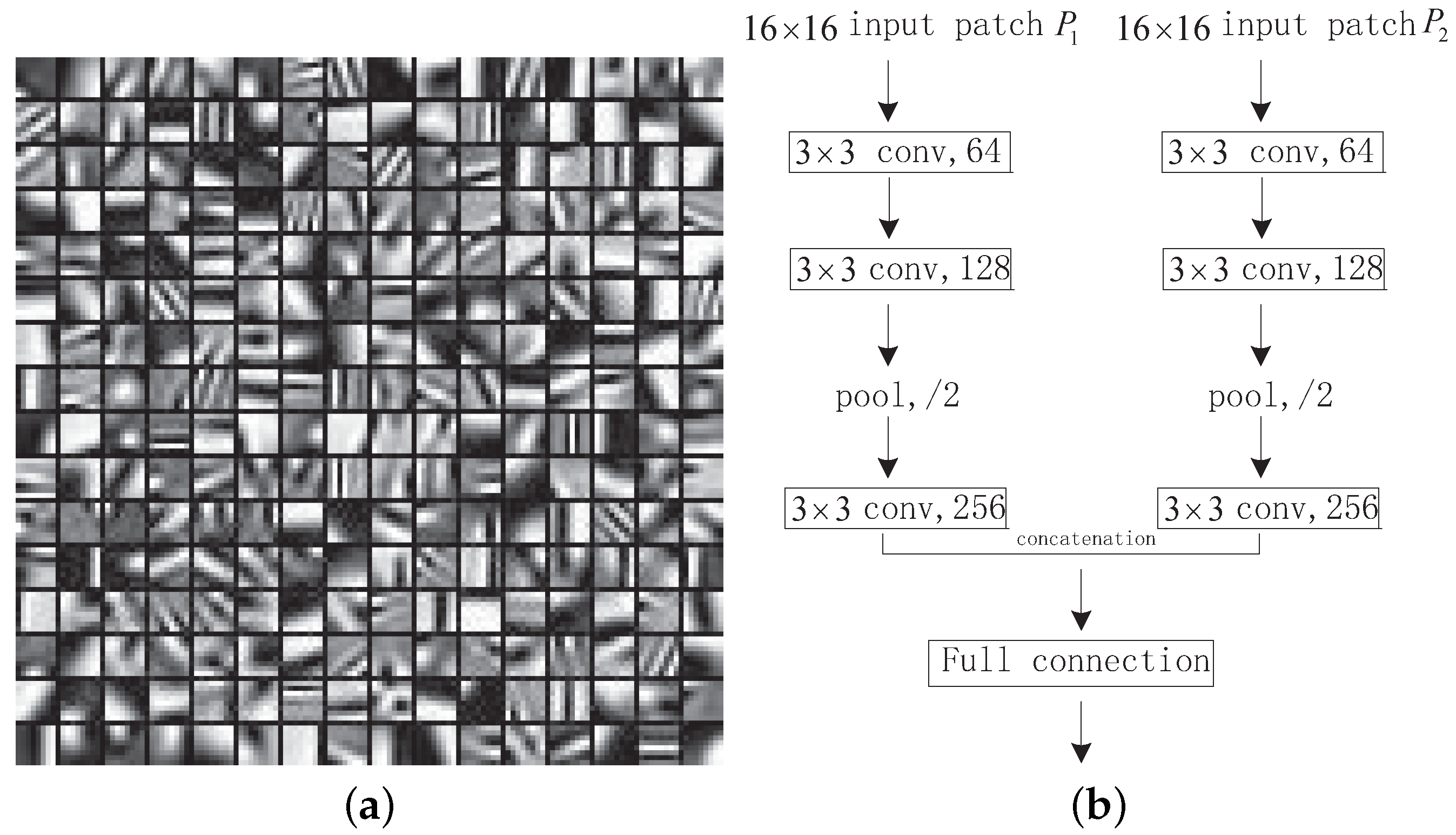
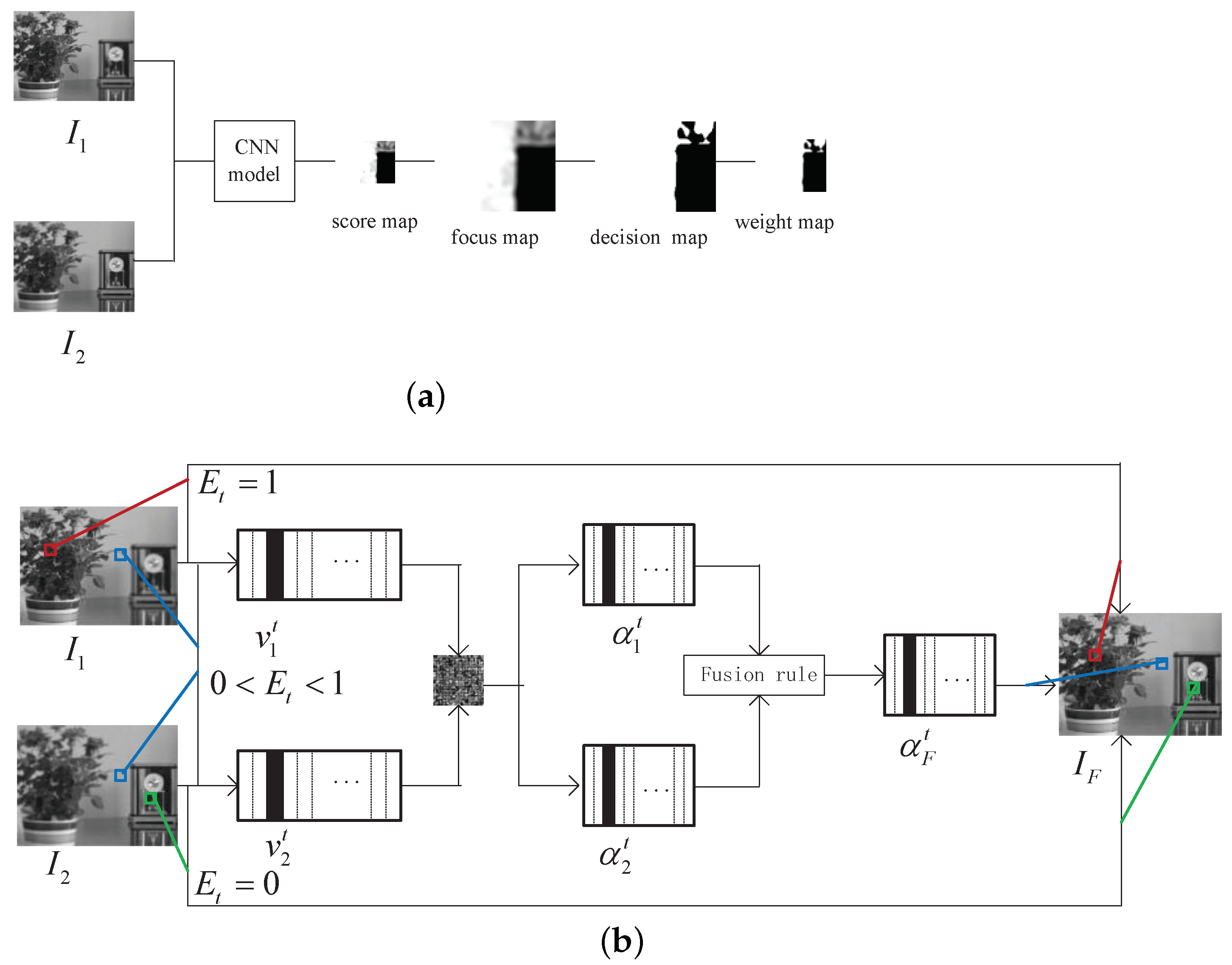
2.2. CNN-Based Image Fusion Method
| Algorithm 1 Dictionary Learning (K-SVD) |
|
2.3. Complementary of the Two Methods
3. Proposed Fusion Algorithm
3.1. CNN-Based Weight Map Generation
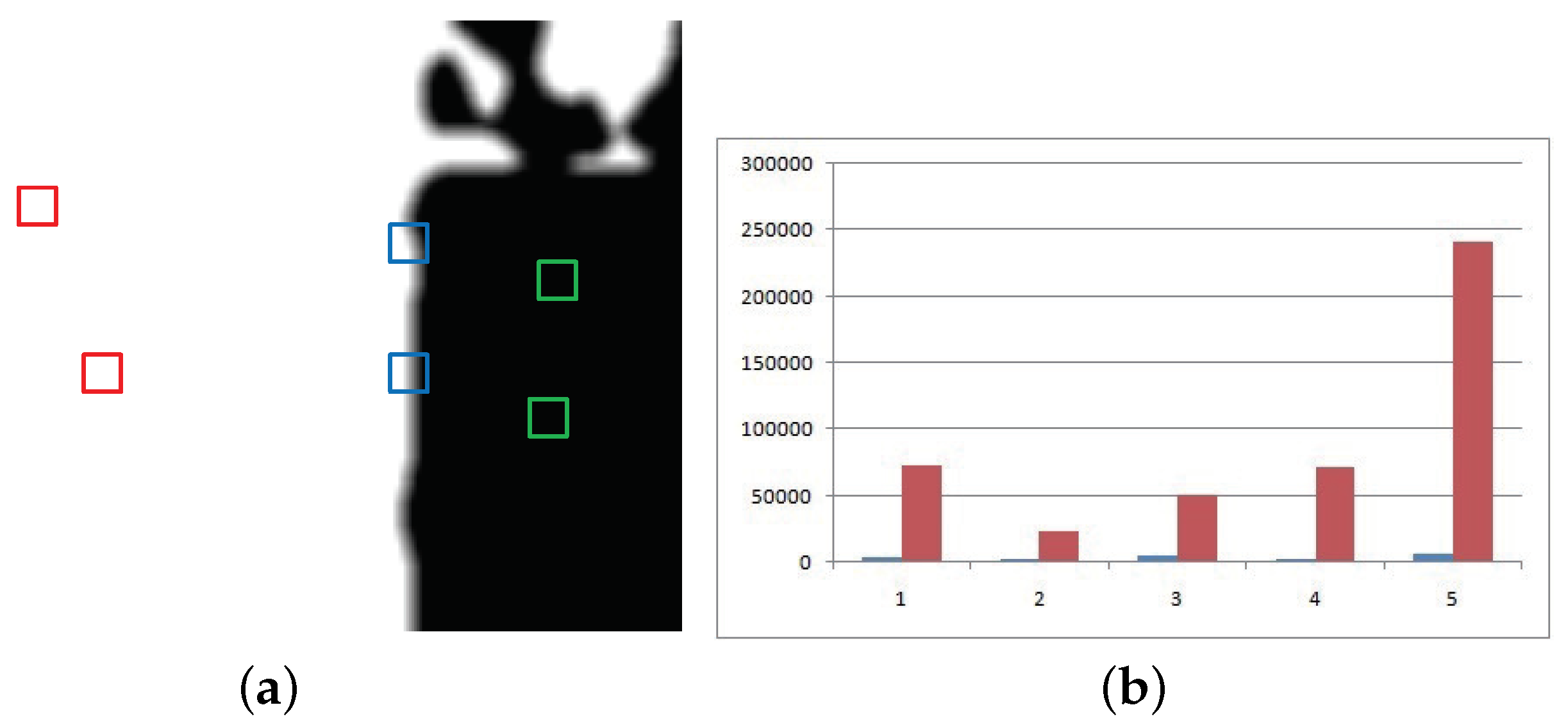
3.2. Fusion of Image Patches Based on the New SR
3.3. Fast Image Fusion Based on Patches
4. Experiments
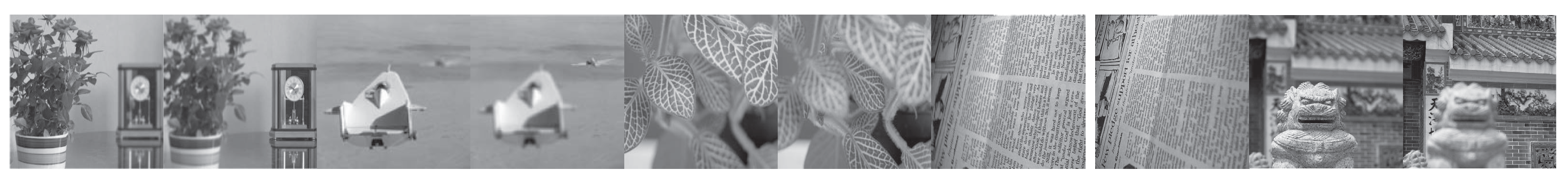
4.1. Source Images
4.2. Evaluation Metrics
- 1.
- Mutual information mainly reflects how much information the fused image contains from the source images [31]. The greater the mutual information is, the more information of the source images the fused image contains, and the better the fusion effect is. Mutual information is defined as follows:Here, are, respectively, the edge histogram of . are normalized joint histograms of and source images , respectively.
- 2.
- The Chen–Blum metric is a human perception-inspired fusion metric. is calculated by the following steps.At the very start, the masked contrast map for the input image can be computed in:where C is Peli’s contrast, are real scalar parameters, and more details on the parameter settings can be found in [32].The information preservation value and the saliency map can be calculated by the two following expressions:Then, the value of the global quality map can be calculated:where is the average of .
- 3.
- The fusion metric based on the gradient is a popular fusion metric which computes the amount of gradient information of the source images injected into the fused image [33]. It is calculated bywhere and are the edge strength and orientation reservation values, respectively. The weight factor shows the significance of .
- 4.
- The fusion metric based on phase congruency measures the image-salient features of the source images, such as the edges and corners in the fused image [34]. The definition of is:where refer to phase congruency, maximum and minimum moments, respectively. The exponential parameters are all set to 1. More details about can be seen in [34].
- 5.
- was proposed by Yang et al., which is a structural similarity-based method of fusion assessment [35]. The definition of is shown as follows:
4.3. Parameters Setting
4.4. The Compared Methods
4.5. Computational Complexity Analysis
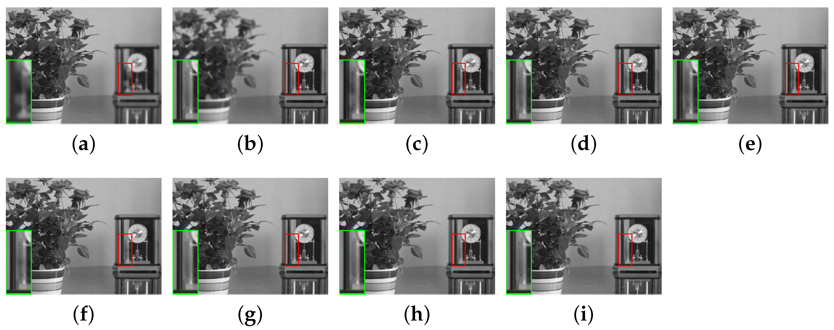
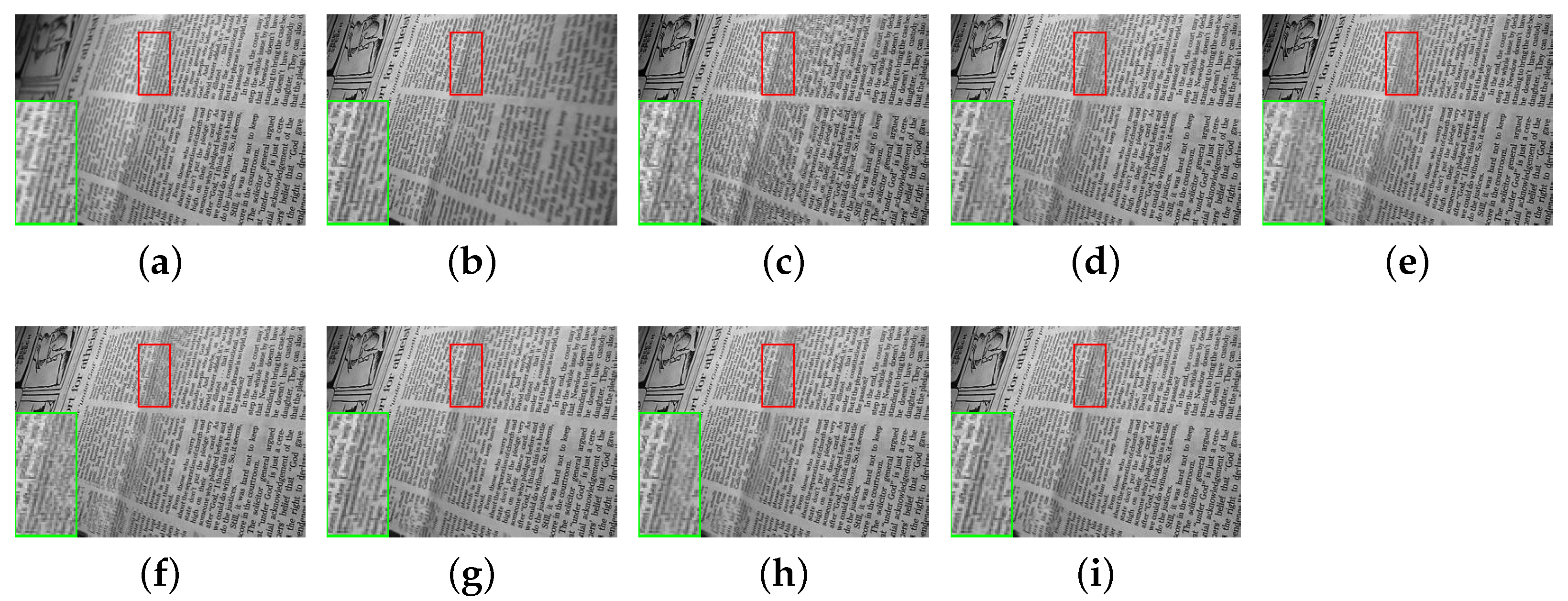
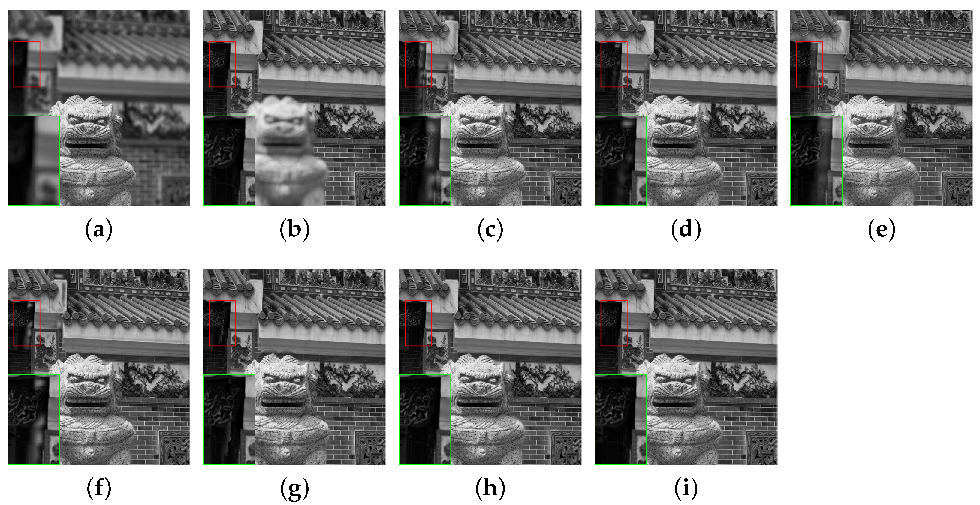
4.6. Validity of the Proposed Fusion Method
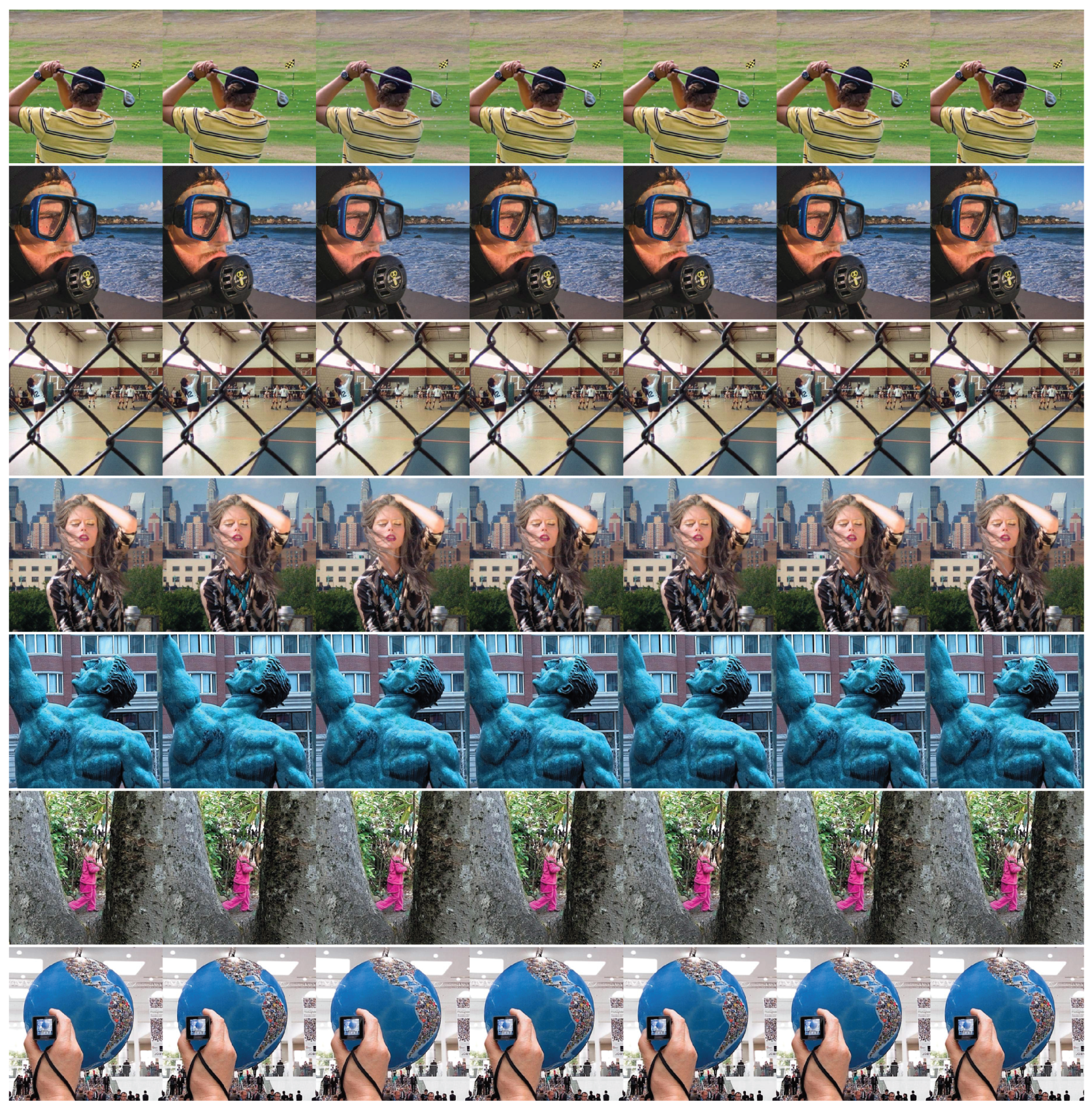
4.7. Fusion of Multi-Focus Color Images
5. Conclusions
Author Contributions
Funding
Data Availability Statement
Conflicts of Interest
References
- Meher, B.; Agrawal, S.; Panda, R.; Abraham, A. A survey on region based image fusion methods. Inf. Fusion 2019, 48, 119–132. [Google Scholar] [CrossRef]
- Guo, L.L.; Woźniak, M. An image super-resolution reconstruction method with single frame character based on wavelet neural network in internet of things. Mob. Netw. Appl. 2021, 26, 390–403. [Google Scholar] [CrossRef]
- Woźniak, M.; Polap, D. Soft trees with neural components as image-processing technique for archeological excavations. Pers. Ubiquitous Comput. 2020, 24, 363–375. [Google Scholar] [CrossRef] [Green Version]
- Liu, Y.; Wang, L.; Cheng, J.; Li, C.; Chen, X. Multi-focus image fusion: A survey of the state of the art. Inf. Fusion 2020, 64, 71–91. [Google Scholar] [CrossRef]
- Farid, M.S.; Mahmood, A.; Al-Maadeed, S.A. Multi-focus image fusion using content adaptive blurring. Inf. Fusion 2019, 45, 96–112. [Google Scholar] [CrossRef]
- Panigrahy, C.; Seal, A.; Mahato, N.K. Fractal dimension based parameter adaptive dual channel PCNN for multi-focus image fusion. Opt. Lasers Eng. 2020, 133, 106–141. [Google Scholar] [CrossRef]
- Nejati, M.; Samavi, S.; Shirani, S. Multi-focus image fusion using dictionary-based sparse representation. Inf. Fusion 2015, 25, 72–84. [Google Scholar] [CrossRef]
- Wang, K.P.; Qi, G.Q.; Zhu, Z.Q.; Chai, Y. A novel geometric dictionary construction approach for sparse representation based image fusion. Entropy 2017, 19, 306. [Google Scholar] [CrossRef] [Green Version]
- Yang, B.; Li, S.T. Multifocus image fusion and restoration with sparse representation. IEEE Trans. Instrum. Meas. 2009, 59, 884–892. [Google Scholar] [CrossRef]
- Li, Y.Y.; Sun, Y.J.; Huang, X.H.; Qi, G.Q.; Zheng, M.Y.; Zhu, Z.Q. An image fusion method based on sparse representation and sum modified-Laplacian in NSCT domain. Entropy 2018, 20, 522. [Google Scholar] [CrossRef] [Green Version]
- Li, S.T.; Yin, H.T.; Fang, L.Y. Group-sparse representation with dictionary learning for medical image denoising and fusion. IEEE Trans. Biomed. Eng. 2012, 59, 3450–3459. [Google Scholar] [CrossRef] [PubMed]
- Liu, Y.; Wang, Z.F. Simultaneous image fusion and denoising with adaptive sparse representation. IET Image Process. 2014, 9, 347–357. [Google Scholar] [CrossRef] [Green Version]
- Liu, Y.; Chen, X.; Ward, R.K.; Wang, Z.J. Image Fusion with Convolutional Sparse Representation. IEEE Signal Process. Lett. 2016, 23, 1882–1886. [Google Scholar] [CrossRef]
- Liu, Y.; Chen, X.; Peng, H.; Wang, Z.F. Multi-focus image fusion with a deep convolutional neural network. Inf. Fusion 2017, 36, 191–207. [Google Scholar] [CrossRef]
- Wei, Q.; Bioucas-Dias, J.; Dobigeon, N.; Tourneret, J.Y. Hyperspectral and multispectral image fusion based on a sparse representation. IEEE Trans. Geosci. Remote Sens. 2015, 53, 3658–3668. [Google Scholar] [CrossRef] [Green Version]
- Chen, L.; Li, J.B.; Chen, C.L.P. Regional multifocus image fusion using sparse representation. Opt. Express 2013, 21, 5182–5197. [Google Scholar] [CrossRef]
- Tang, H.; Xiao, B.; Li, W.S.; Wang, G.Y. Pixel convolutional neural network for multi-focus image fusion. Inf. Sci. 2018, 433, 125–141. [Google Scholar] [CrossRef]
- Dian, R.W.; Li, S.T.; Fang, L.Y.; Wei, Q. Multispectral and hyperspectral image fusion with spatial-spectral sparse representation. Inf. Fusion 2019, 49, 262–270. [Google Scholar] [CrossRef]
- Yin, H.P.; Li, Y.X.; Chai, Y.; Liu, Z.D.; Zhu, Z.Q. A novel sparse-representation-based multi-focus image fusion approach. Neurocomputing 2016, 216, 216–229. [Google Scholar] [CrossRef]
- Xu, M.; Hu, D.L.; Luo, F.L.; Liu, F.L.; Wang, S.Y.; Wu, W.W. Limited angle X ray CT reconstruction using image gradient l0 norm with dictionary learning. IEEE Trans. Radiat. Plasma Med. Sci. 2020, 5, 78–87. [Google Scholar] [CrossRef]
- Zhang, J.; Zhao, C.; Zhao, D.B.; Gao, W. Image compressive sensing recovery using adaptively learned sparsifying basis via l0 minimization. Signal Process. 2014, 103, 114–126. [Google Scholar] [CrossRef] [Green Version]
- Cai, T.T.; Wang, L. Orthogonal matching pursuit for sparse signal recovery with noise. IEEE Trans. Inf. Theory 2011, 57, 4680–4688. [Google Scholar] [CrossRef]
- Wang, J.; Kwon, S.; Shim, B. Generalized orthogonal matching pursuit. IEEE Trans. Signal Process. 2012, 60, 6202–6216. [Google Scholar] [CrossRef] [Green Version]
- Jeon, M.J.; Jeong, Y.S. Compact and Accurate Scene Text Detector. Appl. Sci. 2020, 10, 2096. [Google Scholar] [CrossRef] [Green Version]
- Woźniak, M.; Silka, J.; Wieczorek, M. Deep neural network correlation learning mechanism for CT brain tumor detection. Neural Comput. Appl. 2021, 6, 1–16. [Google Scholar]
- Vu, T.; Nguyen, C.V.; Pham, T.X.; Luu, T.M.; Yoo, C.D. Fast and Efficient Image Quality Enhancement via Desubpixel Convolutional Neural Networks. In Proceedings of the European Conference on Computer Vision (ECCV), Munich, Germany, 8–14 September 2018. [Google Scholar]
- Lytro Multi-Focus Dataset. Available online: https://mansournejati.ece.iut.ac.ir/content/lytro-multi-focus-dataset (accessed on 7 December 2020).
- Multi-Focus-Image-Fusion-Dataset. Available online: https://github.com/sametaymaz/Multi-focus-Image-Fusion-Dataset (accessed on 7 December 2020).
- Tsagaris, V. Objective evaluation of color image fusion methods. Opt. Eng. 2009, 46, 066201. [Google Scholar] [CrossRef]
- Petrović, V. Subjective tests for image fusion evaluation and objective metric validation. Inf. Fusion 2007, 8, 208–216. [Google Scholar]
- Zhu, Z.Q.; Yin, H.P.; Chai, Y.; Li, Y.X.; Qi, G.Q. A novel multi-modality image fusion method based on image decomposition and sparse representation. Inf. Sci. 2018, 432, 516–529. [Google Scholar] [CrossRef]
- Chen, Y.; Blum, R.S. A new automated quality assessment algorithm for image fusion. Image Vis. Comput. 2009, 27, 1421–1432. [Google Scholar] [CrossRef]
- Xydeas, C.S.; Petrovic, V.S. Objective image fusion performance measure. Electron. Lett. 2004, 36, 308–309. [Google Scholar] [CrossRef] [Green Version]
- Zhao, J.; Laganiere, R.; Liu, Z. Performance assessment of combinative pixel-level image fusion based on an absolute feature measurement. Int. J. Innov. Comput. 2007, 3, 1433–1447. [Google Scholar]
- Yang, C.; Zhang, J.Q.; Wang, X.R.; Liu, X. A novel similarity based quality metric for image fusion. Inf. Fusion 2008, 9, 156–160. [Google Scholar] [CrossRef]
- Liu, Z.; Blasch, E.; Xue, Z.; Zhao, J.; Laganiere, R.; Wu, W. Objective assessment of multiresolution image fusion algorithms for context enhancement in night vision: A comparative study. IEEE Trans. Pattern Anal. Mach. Intell. 2011, 34, 94–109. [Google Scholar] [CrossRef] [PubMed]
- Zong, J.J.; Qiu, T.S. Medical image fusion based on sparse representation of classified image patches. Biomed. Signal Process. Control 2017, 34, 195–205. [Google Scholar] [CrossRef]
- Liu, Y.; Liu, S.; Wang, Z. A general framework for image fusion based on multi-scale transform and sparse representation. Inf. Fusion 2017, 24, 147–164. [Google Scholar] [CrossRef]


| Image | Flowerpot | Aircraft | Leaf | Newspaper | Temple |
|---|---|---|---|---|---|
| SR | 165.6602 | 51.6356 | 118.1120 | 168.7816 | 578.9371 |
| CNN | 143.2177 | 68.1374 | 125.2807 | 148.8524 | 319.9401 |
| CNN-SR | 105.2181 | 47.8837 | 91.1454 | 102.0202 | 265.0994 |
| Metric | MST | SR | ASR | MST-SR | CSR | CNN | CNN-SR |
|---|---|---|---|---|---|---|---|
| MI | 0.9463 | 1.1033 | 0.9587 | 1.0777 | 0.9837 | 1.1656 | 1.1754 |
| 0.7083 | 0.7256 | 0.7285 | 0.7332 | 0.7149 | 0.7490 | 0.7463 | |
| 0.6118 | 0.6116 | 0.6123 | 0.6225 | 0.5492 | 0.6461 | 0.6480 | |
| 0.8996 | 0.9220 | 0.9117 | 0.9207 | 0.9164 | 0.9239 | 0.9239 | |
| 0.9490 | 0.9469 | 0.9508 | 0.9539 | 0.8837 | 0.9728 | 0.9756 |
| Metric | MST | SR | ASR | MST-SR | CSR | CNN | CNN-SR |
|---|---|---|---|---|---|---|---|
| MI | 1.1138 | 1.2690 | 1.1585 | 1.2436 | 1.1774 | 1.3457 | 1.3575 |
| 0.7115 | 0.7182 | 0.6855 | 0.7202 | 0.6692 | 0.7547 | 0.7596 | |
| 0.5990 | 0.6237 | 0.5975 | 0.6213 | 0.4985 | 0.6670 | 0.6727 | |
| 0.7522 | 0.7627 | 0.7580 | 0.7643 | 0.7062 | 0.7882 | 0.7915 | |
| 0.9089 | 0.9294 | 0.9154 | 0.9217 | 0.8515 | 0.9728 | 0.9777 |
| Metric | MST | SR | ASR | MST-SR | CSR | CNN | CNN-SR |
|---|---|---|---|---|---|---|---|
| MI | 0.6697 | 0.9286 | 0.6878 | 0.9285 | 0.8012 | 0.9055 | 1.0012 |
| 0.7463 | 0.7691 | 0.7249 | 0.7777 | 0.7747 | 0.7812 | 0.7905 | |
| 0.6527 | 0.6648 | 0.6561 | 0.6744 | 0.6381 | 0.6822 | 0.6871 | |
| 0.8121 | 0.8360 | 0.8207 | 0.8360 | 0.8307 | 0.8456 | 0.8409 | |
| 0.9569 | 0.9660 | 0.9601 | 0.9703 | 0.9480 | 0.9845 | 0.9894 |
| Metric | MST | SR | ASR | MST-SR | CSR | CNN | CNN-SR |
|---|---|---|---|---|---|---|---|
| MI | 0.2916 | 0.7365 | 0.3290 | 0.6094 | 0.5955 | 0.7975 | 0.8579 |
| 0.6639 | 0.7282 | 0.6865 | 0.7094 | 0.7337 | 0.7403 | 0.7462 | |
| 0.5876 | 0.6332 | 0.6142 | 0.6150 | 0.6342 | 0.6434 | 0.6513 | |
| 0.4900 | 0.6256 | 0.5959 | 0.6012 | 0.6459 | 0.6449 | 0.6453 | |
| 0.9371 | 0.9781 | 0.9677 | 0.9586 | 0.9854 | 0.9866 | 0.9932 |
| Metric | MST | SR | ASR | MST-SR | CSR | CNN | CNN-SR |
|---|---|---|---|---|---|---|---|
| MI | 0.4136 | 0.8377 | 0.4172 | 0.8163 | 0.7003 | 0.8977 | 0.9388 |
| 0.6809 | 0.7845 | 0.6421 | 0.7739 | 0.7928 | 0.8064 | 0.8102 | |
| 0.6510 | 0.7045 | 0.6452 | 0.7077 | 0.6901 | 0.7168 | 0.7197 | |
| 0.6428 | 0.7840 | 0.6577 | 0.7653 | 0.7734 | 0.7920 | 0.7947 | |
| 0.9356 | 0.9756 | 0.9355 | 0.9675 | 0.9742 | 0.9928 | 0.9951 |
| Metric | MST | SR | ASR | MST-SR | CSR | CNN | CNN-SR |
|---|---|---|---|---|---|---|---|
| MI | 0.9237 | 1.0558 | 0.9219 | 1.0900 | 0.9601 | 1.1105 | 1.1459 |
| 0.7629 | 0.7845 | 0.7426 | 0.8009 | 0.7758 | 0.8105 | 0.8142 | |
| 0.6918 | 0.7036 | 0.6979 | 0.7131 | 0.6547 | 0.7187 | 0.7209 | |
| 0.8326 | 0.8329 | 0.8322 | 0.8447 | 0.8327 | 0.8478 | 0.8471 | |
| 0.9663 | 0.9730 | 0.9699 | 0.9776 | 0.9444 | 0.9847 | 0.9869 |
Publisher’s Note: MDPI stays neutral with regard to jurisdictional claims in published maps and institutional affiliations. |
© 2021 by the authors. Licensee MDPI, Basel, Switzerland. This article is an open access article distributed under the terms and conditions of the Creative Commons Attribution (CC BY) license (https://creativecommons.org/licenses/by/4.0/).
Share and Cite
Wei, B.; Feng, X.; Wang, K.; Gao, B. The Multi-Focus-Image-Fusion Method Based on Convolutional Neural Network and Sparse Representation. Entropy 2021, 23, 827. https://doi.org/10.3390/e23070827
Wei B, Feng X, Wang K, Gao B. The Multi-Focus-Image-Fusion Method Based on Convolutional Neural Network and Sparse Representation. Entropy. 2021; 23(7):827. https://doi.org/10.3390/e23070827
Chicago/Turabian StyleWei, Bingzhe, Xiangchu Feng, Kun Wang, and Bian Gao. 2021. "The Multi-Focus-Image-Fusion Method Based on Convolutional Neural Network and Sparse Representation" Entropy 23, no. 7: 827. https://doi.org/10.3390/e23070827
APA StyleWei, B., Feng, X., Wang, K., & Gao, B. (2021). The Multi-Focus-Image-Fusion Method Based on Convolutional Neural Network and Sparse Representation. Entropy, 23(7), 827. https://doi.org/10.3390/e23070827