Figure 1.
Variance (on the
left) and kurtosis (on the
right) for LS distribution (given by (
5)) as a function of
and
d.
Figure 1.
Variance (on the
left) and kurtosis (on the
right) for LS distribution (given by (
5)) as a function of
and
d.
Figure 2.
Probability density functions of the LS distribution for different values of and d.
Figure 2.
Probability density functions of the LS distribution for different values of and d.
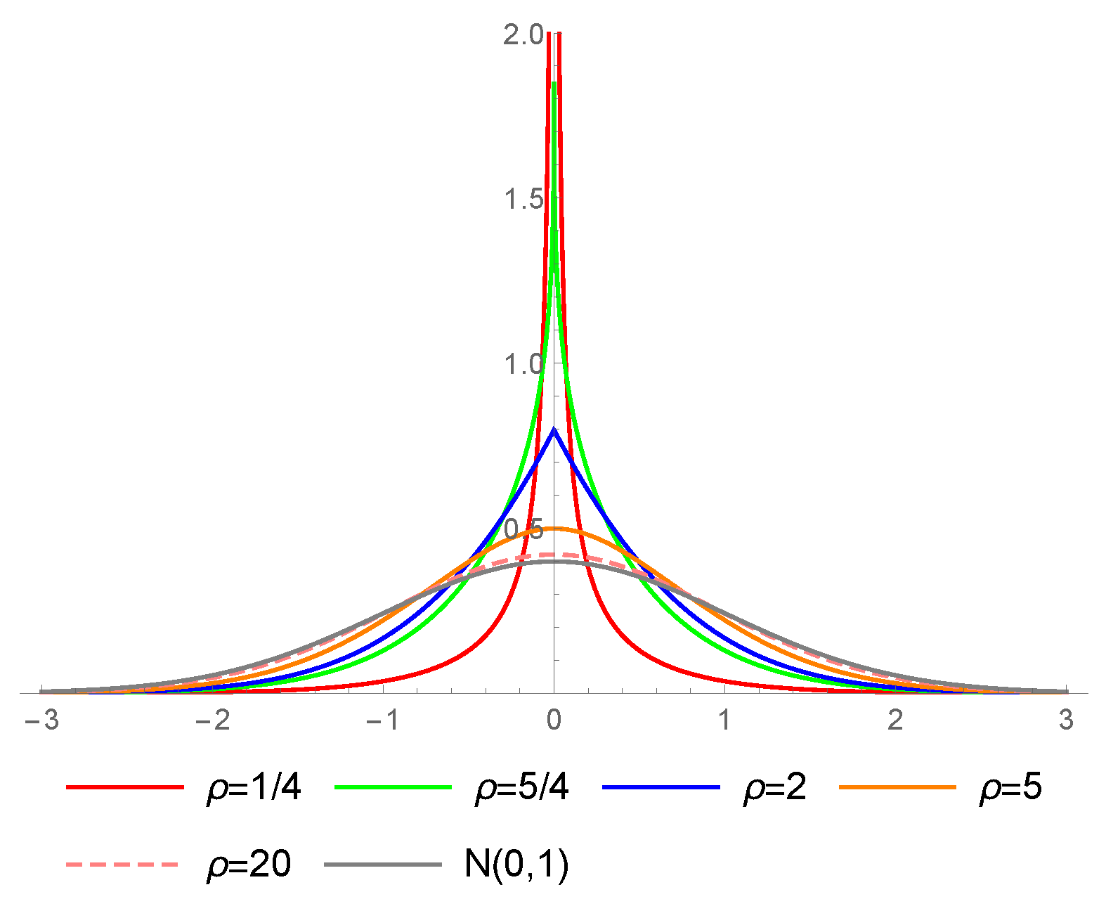
Figure 3.
Probability density functions of the MN type I distribution for different values of .
Figure 3.
Probability density functions of the MN type I distribution for different values of .
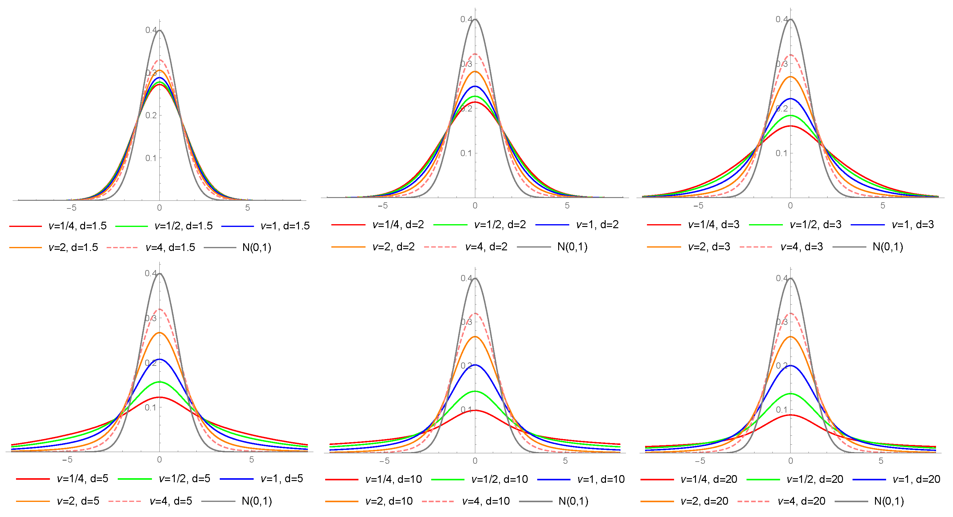
Figure 4.
Probability density functions of the LMN type I distribution for different values of , .
Figure 4.
Probability density functions of the LMN type I distribution for different values of , .
Figure 5.
Probability density functions of the LMN type I distribution for different values of , .
Figure 5.
Probability density functions of the LMN type I distribution for different values of , .
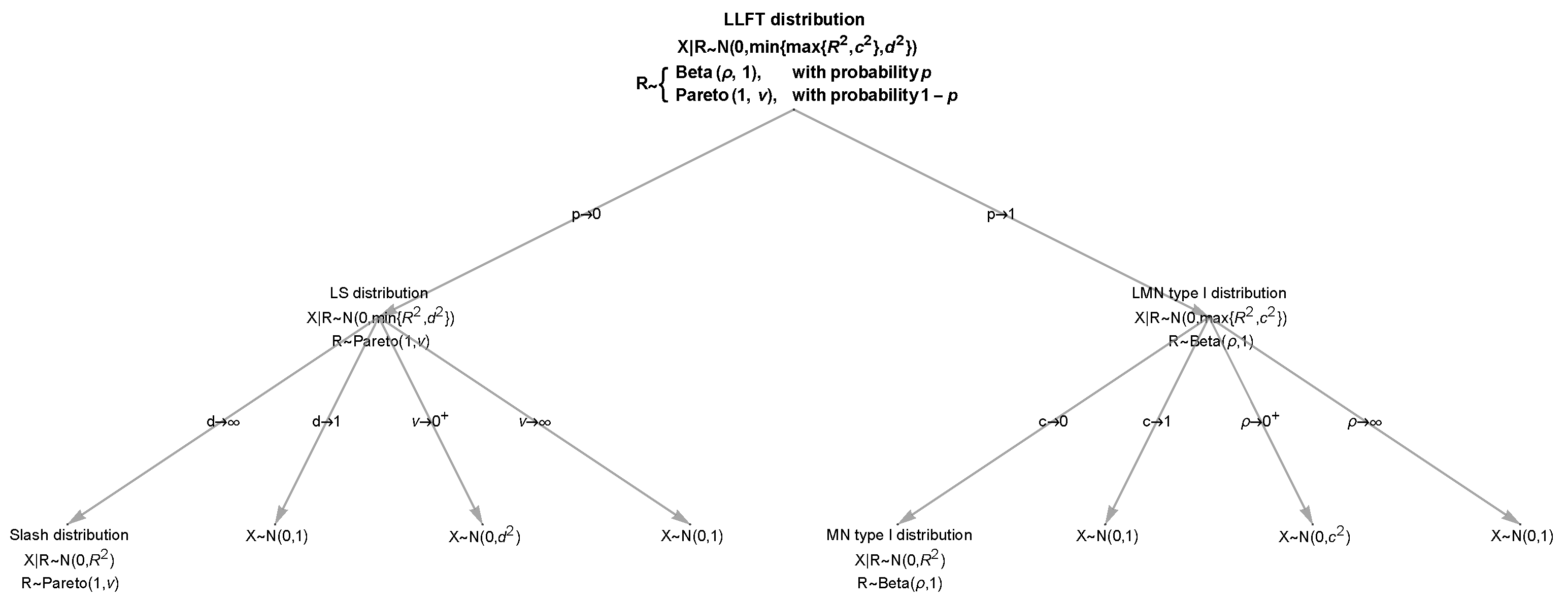
Figure 6.
The tree with limiting cases for the LLFT distribution.
Figure 6.
The tree with limiting cases for the LLFT distribution.
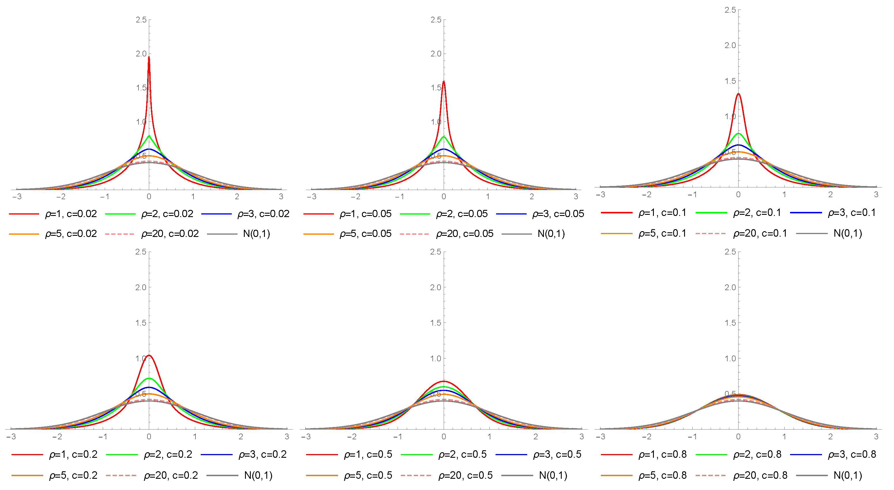
Figure 7.
The pdf of the LLFT distribution for different values of parameters c and d and fixed , and .
Figure 7.
The pdf of the LLFT distribution for different values of parameters c and d and fixed , and .
Figure 8.
Time plots of (a) daily prices, (b) log returns in percentages for MSAG.DE, (c) histogram of log returns (in percentages) for MSAG.DE with a Gaussian curve.
Figure 8.
Time plots of (a) daily prices, (b) log returns in percentages for MSAG.DE, (c) histogram of log returns (in percentages) for MSAG.DE with a Gaussian curve.
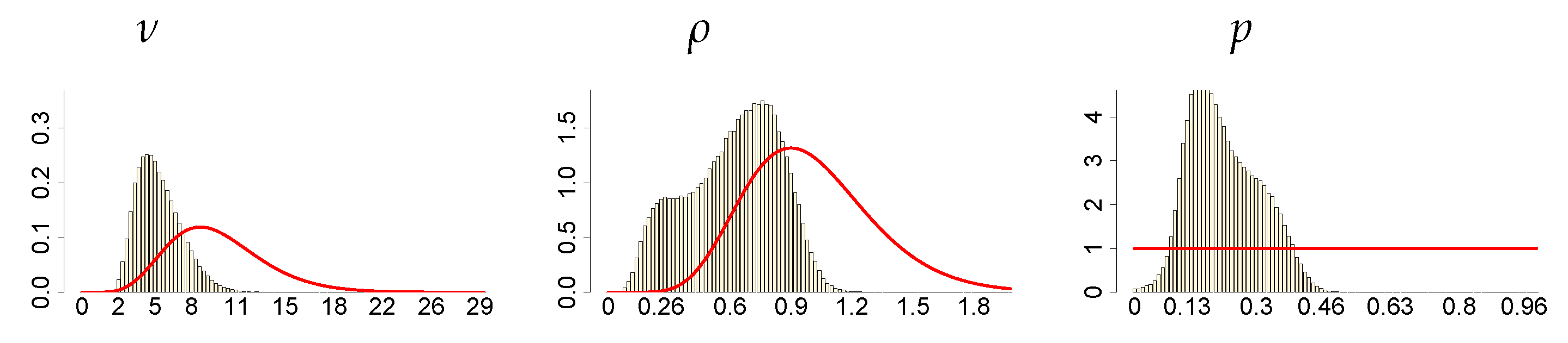
Figure 9.
Histograms of the marginal posteriors (bars) and priors (red line) of mixture parameters , and p, under , and .
Figure 9.
Histograms of the marginal posteriors (bars) and priors (red line) of mixture parameters , and p, under , and .
Figure 10.
Histograms of the marginal posteriors (bars) and priors (red line) of SV parameters , and , under , and .
Figure 10.
Histograms of the marginal posteriors (bars) and priors (red line) of SV parameters , and , under , and .
Figure 11.
Histograms of the marginal posteriors (bars) and priors (red line) of c and d, under , and .
Figure 11.
Histograms of the marginal posteriors (bars) and priors (red line) of c and d, under , and .
Figure 12.
Histograms of the marginal posteriors (bars) and priors (red line) of c and d, under , and .
Figure 12.
Histograms of the marginal posteriors (bars) and priors (red line) of c and d, under , and .
Figure 13.
Bivariate marginal posteriors: (a) for pairs and , (b) for pairs and ; obtained in the LLFT-SV model with , and .
Figure 13.
Bivariate marginal posteriors: (a) for pairs and , (b) for pairs and ; obtained in the LLFT-SV model with , and .
Figure 14.
Bivariate marginal posteriors for pairs and , obtained in the LLFT-SV model with (a) , , , (b) , , , (c) , , .
Figure 14.
Bivariate marginal posteriors for pairs and , obtained in the LLFT-SV model with (a) , , , (b) , , , (c) , , .
Figure 15.
Posterior means (black line) with two standard-deviation bands (truncated only to positive values; red) of s obtained in the LLFT-SV model with: (a) , , , (b) , , , (c) , , .
Figure 15.
Posterior means (black line) with two standard-deviation bands (truncated only to positive values; red) of s obtained in the LLFT-SV model with: (a) , , , (b) , , , (c) , , .
Figure 16.
Posterior means (black line) with two standard-deviation bands (truncated only to positive values; red) of s obtained in the t-SV model with: (a) , (b) .
Figure 16.
Posterior means (black line) with two standard-deviation bands (truncated only to positive values; red) of s obtained in the t-SV model with: (a) , (b) .
Figure 17.
Posterior means (black line) with two-standard-deviation bands (truncated only to positive values; red) obtained in the LLFT-SV model with , , for: (a) , (b) .
Figure 17.
Posterior means (black line) with two-standard-deviation bands (truncated only to positive values; red) obtained in the LLFT-SV model with , , for: (a) , (b) .
Figure 18.
Posterior means (black lines) with two-stsandard-deviation bands (truncated only to positive values; red) of , obtained in the LLFT-SV model with , , and: (a) , (b) .
Figure 18.
Posterior means (black lines) with two-stsandard-deviation bands (truncated only to positive values; red) of , obtained in the LLFT-SV model with , , and: (a) , (b) .
Figure 19.
Posterior means (black line) with two-standard-deviation bands (truncated only to positive values; red) of obtained in the t-SV model with: (a) , (b) .
Figure 19.
Posterior means (black line) with two-standard-deviation bands (truncated only to positive values; red) of obtained in the t-SV model with: (a) , (b) .
Figure 20.
Posterior means (black line) with two-standard-deviation bands (truncated only to positive values; red) of obtained in the LLFT-SV model with: (a) , , , (b) , , , (c) , , . (d) The series of modelled returns.
Figure 20.
Posterior means (black line) with two-standard-deviation bands (truncated only to positive values; red) of obtained in the LLFT-SV model with: (a) , , , (b) , , , (c) , , . (d) The series of modelled returns.
Figure 21.
Posterior means (black line) with two-standard-deviation bands (truncated only to positive values; red) of obtained in the t-SV model with: (a) , (b) . (c) The series of modelled returns.
Figure 21.
Posterior means (black line) with two-standard-deviation bands (truncated only to positive values; red) of obtained in the t-SV model with: (a) , (b) . (c) The series of modelled returns.
Figure 22.
Bivariate marginal posteriors for pairs and , obtained in the LLFT-SV model, under , and ; (a) for the original MSAG.DE data set, (b) for the perturbed data, , (c) for the perturbed data, .
Figure 22.
Bivariate marginal posteriors for pairs and , obtained in the LLFT-SV model, under , and ; (a) for the original MSAG.DE data set, (b) for the perturbed data, , (c) for the perturbed data, .
Figure 23.
Posterior means (black line) with two-standard-deviation bands (truncated only to positive values; red) of obtained for the original MSAG.DE data in the LLFT-SV model with , and: (a) , (b) .
Figure 23.
Posterior means (black line) with two-standard-deviation bands (truncated only to positive values; red) of obtained for the original MSAG.DE data in the LLFT-SV model with , and: (a) , (b) .
Figure 24.
Posterior means (black line) with two-standard-deviation bands (truncated only to positive values; red) of , obtained for the original MSAG.DE data in the LLFT-SV model with , and: (a) , (b) .
Figure 24.
Posterior means (black line) with two-standard-deviation bands (truncated only to positive values; red) of , obtained for the original MSAG.DE data in the LLFT-SV model with , and: (a) , (b) .
Figure 25.
Posterior means (black line) with two-standard-deviation bands (truncated only to positive values; red) of , obtained in the LLFT-SV model for the perturbed MSAG.DE data. The prior distribution: , . The result for: (a) the first perturbation, (b) the second perturbation.
Figure 25.
Posterior means (black line) with two-standard-deviation bands (truncated only to positive values; red) of , obtained in the LLFT-SV model for the perturbed MSAG.DE data. The prior distribution: , . The result for: (a) the first perturbation, (b) the second perturbation.
Figure 26.
The series (left) and histograms (with fitted Gaussian curves; right) of the S&P 500 and DAX returns.
Figure 26.
The series (left) and histograms (with fitted Gaussian curves; right) of the S&P 500 and DAX returns.
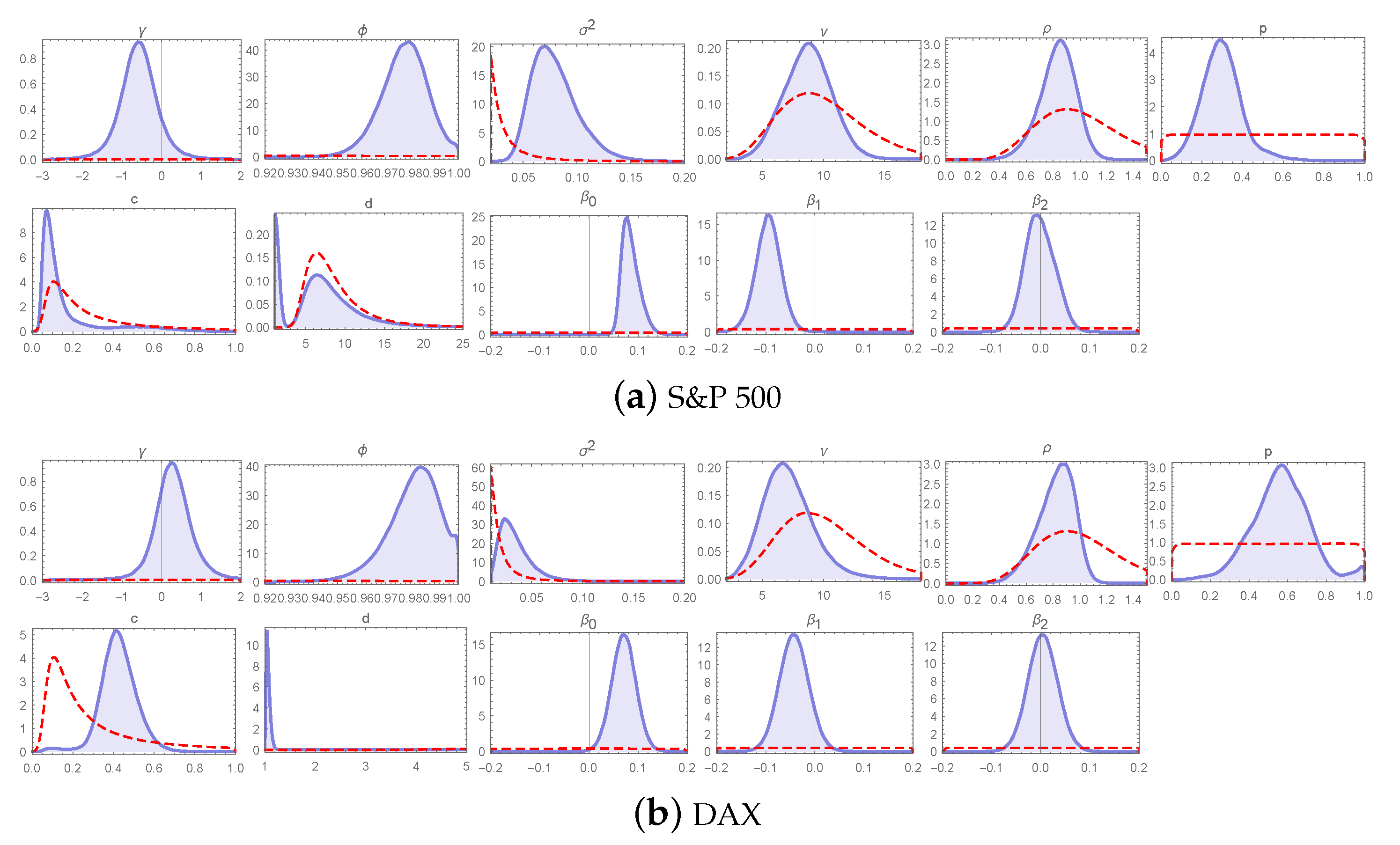
Figure 27.
Marginal posteriors (blue line) and priors (red line) of the LLFT-SV model parameters under , and . The top two rows show plots for S&P 500 and the bottom two rows for DAX.
Figure 27.
Marginal posteriors (blue line) and priors (red line) of the LLFT-SV model parameters under , and . The top two rows show plots for S&P 500 and the bottom two rows for DAX.
Table 1.
Sample characteristics for the MSAG.DE data set.
Table 1.
Sample characteristics for the MSAG.DE data set.
| Mean | St. Dev. | Median | Min | Max | Skewness | Kurtosis | Percent of Zero Returns |
|---|
| | | | | | | |
Table 2.
Posterior characteristics of model parameters for the original MSAG.DE data set. The first row of each entry: posterior median. The second row: 90% posterior confidence interval (in parentheses). The third row: interquartile range.
Table 2.
Posterior characteristics of model parameters for the original MSAG.DE data set. The first row of each entry: posterior median. The second row: 90% posterior confidence interval (in parentheses). The third row: interquartile range.
| Parameter | LLFT-SV | LLFT-SV | LLFT-SV | t-SV | t-SV |
|---|
| | | | | | |
| | | | | – | – |
| | | | | – | – |
| 0.947 | 1.290 | 1.206 | 0.982 | 1.045 |
| | (0.492, 1.500) | (0.772, 1.682) | (0.758, 1.661) | (0.709, 1.255) | (0.779, 1.304) |
| | 0.406 | 0.413 | 0.392 | 0.224 | 0.210 |
| 0.914 | 0.905 | 0.911 | 0.905 | 0.899 |
| | (0.860, 0.950) | (0.854, 0.944) | (0.860, 0.947) | (0.851, 0.947) | (0.839, 0.941) |
| | 0.036 | 0.036 | 0.036 | 0.036 | 0.042 |
| 0.150 | 0.171 | 0.156 | 0.156 | 0.186 |
| | (0.078, 0.261) | (0.099, 0.282) | (0.087, 0.270) | (0.087, 0.282) | (0.102, 0.324) |
| | 0.072 | 0.072 | 0.069 | 0.078 | 0.087 |
| 3.99 | 6.30 | 5.60 | 5.11 | 6.44 |
| | (2.73, 7.35) | (3.64, 8.82) | (3.57, 8.96) | (3.64, 8.54) | (4.34, 10.85) |
| | 1.82 | 2.38 | 2.24 | 1.68 | 2.52 |
| 0.64 | 0.67 | 0.66 | – | – |
| | (0.22, 0.98) | (0.24, 0.97) | (0.23, 0.96) | – | – |
| | 0.33 | 0.32 | 0.35 | – | – |
| p | 0.148 | 0.240 | 0.214 | – | – |
| | (0.046, 0.302) | (0.106, 0.363) | (0.107, 0.382) | – | – |
| | 0.087 | 0.125 | 0.131 | – | – |
| c | 0.134 | 0.120 | 0.118 | – | – |
| | (0.061, 0.261) | (0.058, 0.231) | (0.057, 0.220) | – | – |
| | 0.077 | 0.067 | 0.067 | – | – |
| d | 5.161 | 3.354 | 7.553 | – | – |
| | (1.144, 10.673) | (1.105, 6.396) | (1.105, 16.632) | – | – |
| | 2.951 | 3.146 | 4.524 | – | – |
| −0.043 | −0.040 | −0.037 | −0.076 | −0.082 |
| | (−0.130, 0.008) | (−0.121, 0.008) | (−0.118, 0.008) | (−0.163, 0.008) | (−0.166, 0.005) |
| | 0.066 | 0.063 | 0.060 | 0.069 | 0.069 |
| −0.046 | -0.037 | −0.034 | −0.115 | −0.118 |
| | (−0.118, 0.005) | (−0.100, 0.005) | (−0.097, 0.005) | (−0.163, −0.067) | (−0.166, −0.067) |
| | 0.060 | 0.048 | 0.051 | 0.042 | 0.039 |
| 0.023 | 0.023 | 0.023 | 0.035 | 0.035 |
| | (−0.004, 0.065) | (−0.001, 0.065) | (−0.001, 0.062) | (−0.010, 0.080) | (−0.010, 0.083) |
| | 0.030 | 0.030 | 0.027 | 0.036 | 0.039 |
Table 3.
Basic characteristics (averages, standard deviations, correlation coefficients) of the posterior means of latent processes, in models with , , and .
Table 3.
Basic characteristics (averages, standard deviations, correlation coefficients) of the posterior means of latent processes, in models with , , and .
| Latent Process | Model Type | Average | Standard Deviation | Correlation Coefficient |
|---|
| LLFT-SV | 5.865 | 9.126 | 0.994 |
| | t-SV | 4.854 | 6.710 | |
| LLFT-SV | 1.071 | 0.234 | 0.759 |
| t-SV | 1.148 | 0.154 | |
| LLFT-SV | 2.119 | 1.051 | 0.964 |
| t-SV | 2.173 | 1.210 | |
Table 4.
Sums of the log predictive likelihoods.
Table 4.
Sums of the log predictive likelihoods.
| Forecast | LLFT-SV | LLFT-SV | t-SV |
|---|
| Horizon | | | |
|---|
| | | |
| | | |
| | | |
| | | |
| | | |
| | | |
| | | |
| | | |
| | | |
| | | |
Table 5.
Posterior characteristics of model parameters for the perturbed and original MSAG.DE data, under . The first row of each entry: posterior median. The second row: 90% posterior confidence interval (in parentheses). The third row: interquartile range.
Table 5.
Posterior characteristics of model parameters for the perturbed and original MSAG.DE data, under . The first row of each entry: posterior median. The second row: 90% posterior confidence interval (in parentheses). The third row: interquartile range.
| Parameter | Original Data | Perturbed Data | Original Data | Perturbed Data |
|---|
| | LLFT-SV | LLFT-SV | t-SV | t-SV |
|---|
| | | | | |
| | | | | |
| | | | – | – |
| | | | – | – |
| 1.206 | 1.227 | 1.045 | 1.045 |
| | (0.758, 1.661) | (0.800, 1.654) | (0.779, 1.304) | (0.786, 1.304) |
| | 0.392 | 0.371 | 0.210 | 0.210 |
| 0.911 | 0.914 | 0.899 | 0.902 |
| | (0.860, 0.947) | (0.863, 0.950) | (0.839, 0.941) | (0.842, 0.944) |
| | 0.036 | 0.033 | 0.042 | 0.039 |
| 0.156 | 0.150 | 0.186 | 0.177 |
| | (0.087, 0.270) | (0.084, 0.255) | (0.102, 0.324) | (0.096, 0.309) |
| | 0.069 | 0.066 | 0.087 | 0.087 |
| 5.60 | 5.67 | 6.44 | 6.44 |
| | (3.57, 8.96) | (3.71, 8.89) | (4.34, 10.85) | (4.34, 10.71) |
| | 2.24 | 2.17 | 2.52 | 2.45 |
| 0.66 | 0.70 | – | – |
| | (0.23, 0.96) | (0.35, 0.97) | – | – |
| | 0.35 | 0.26 | – | – |
| p | 0.214 | 0.226 | – | – |
| | (0.107, 0.382) | (0.109, 0.381) | – | – |
| | 0.131 | 0.126 | – | – |
| c | 0.118 | 0.127 | – | – |
| | (0.057, 0.220) | (0.072, 0.229) | – | – |
| | 0.067 | 0.057 | – | – |
| d | 7.553 | 7.462 | – | – |
| | (1.105, 16.632) | (1.118, 16.376) | – | – |
| | 4.524 | 4.472 | – | – |
| −0.037 | −0.049 | −0.082 | −0.079 |
| | (−0.118, 0.008) | (−0.124, 0.005) | (−0.166, 0.005) | (−0.166, 0.005) |
| | 0.060 | 0.054 | 0.069 | 0.069 |
| −0.034 | −0.043 | −0.118 | −0.118 |
| | (−0.097, 0.005) | (−0.100, −0.001) | (−0.166, −0.067) | (−0.166, −0.067) |
| | 0.051 | 0.042 | 0.039 | 0.039 |
| 0.023 | 0.029 | 0.035 | 0.038 |
| | (−0.001, 0.062) | (−0.001, 0.065) | (−0.010, 0.083) | (−0.010, 0.086) |
| | 0.027 | 0.027 | 0.039 | 0.036 |
Table 6.
Posterior characteristics of the LLFT-SV model parameters for the perturbed and original MSAG.DE data, under . The first row of each entry: posterior median. The second row: 90% posterior confidence interval (in parentheses). The third row: interquartile range.
Table 6.
Posterior characteristics of the LLFT-SV model parameters for the perturbed and original MSAG.DE data, under . The first row of each entry: posterior median. The second row: 90% posterior confidence interval (in parentheses). The third row: interquartile range.
| Parameter | Perturbed Data | Perturbed Data | Original Data |
|---|
| | | | |
| | | | |
| | | | |
| 0.800 | −0.005 | −0.047 |
| | (0.408, 1.129) | (−0.278, 0.387) | (−0.306, 0.219) |
| | 0.273 | 0.231 | 0.211 |
| 0.929 | 0.917 | 0.911 |
| | (0.881, 0.962) | (0.866, 0.950) | (0.860, 0.947) |
| | 0.033 | 0.033 | 0.033 |
| 0.102 | 0.135 | 0.153 |
| | (0.048, 0.183) | (0.081, 0.225) | (0.090, 0.255) |
| | 0.054 | 0.057 | 0.066 |
| 3.36 | 1.040 | 1.032 |
| | (1.47, 4.83) | (1.003, 2.394) | (1.002, 1.133) |
| | 0.98 | 0.07 | 0.05 |
| 0.11 | 0.047 | 0.046 |
| | (0.06, 0.17) | (0.027, 0.079) | (0.029, 0.078) |
| | 0.04 | 0.02 | 0.020 |
| p | 0.119 | 0.1170 | 0.117 |
| | (0.097, 0.144) | (0.100, 0.136) | (0.100, 0.136) |
| | 0.019 | 0.015 | 0.015 |
| c | 0.021 | 0.014 | 0.014 |
| | (0.018, 0.025) | (0.012, 0.015) | (0.012, 0.016) |
| | 0.002 | 0.001 | 0.001 |
| d | 9.503 | 2.795 | 2.806 |
| | (2.316, 18.985) | (2.496, 10.764) | (2.514, 3.496) |
| | 4.706 | 0.260 | 0.230 |
| −0.002 | −0.0001 | −0.0001 |
| | (−0.007, 0.003) | (−0.0017, 0.001) | (−0.001, 0.002) |
| | 0.003 | 0.001 | 0.001 |
| −0.0003 | −0.0002 | 0.0000 |
| | (−0.003, 0.003) | (−0.0013, 0.0008) | (−0.0004, 0.001) |
| | 0.0025 | 0.0005 | 0.001 |
| 0.0015 | 0.0000 | 0.0000 |
| | (−0.001, 0.0044) | (−0.0009, 0.0011) | (−0.0004, 0.001) |
| | 0.002 | 0.0008 | 0.0007 |
Table 7.
Posterior characteristics of the LLFT-SV model parameters for DAX and S&P 500, under . The first row of each entry: posterior median. The second row: 90% posterior confidence interval (in parentheses). The third row: interquartile range.
Table 7.
Posterior characteristics of the LLFT-SV model parameters for DAX and S&P 500, under . The first row of each entry: posterior median. The second row: 90% posterior confidence interval (in parentheses). The third row: interquartile range.
| Parameter | DAX | DAX | S&P 500 | S&P 500 |
|---|
| | | | | |
| | | | | |
| 0.191 | 0.296 | −0.558 | −572 |
| | (−0.649, 1.080) | (−0.565, 1.269) | (−1.377, 0.289) | (−1.419, 0.303) |
| | 0.560 | 0.588 | 0.581 | 0.588 |
| 0.983 | 0.983 | 0.980 | 0.980 |
| | (0.962, 0.998) | (0.962, 0.998) | (0.962, 0.995) | (0.962, 0.995) |
| | 0.012 | 0.015 | 0.012 | 0.012 |
| 0.033 | 0.033 | 0.081 | 0.078 |
| | (0.018, 0.066) | (0.015, 0.063) | (0.054, 0.120) | (0.051, 0.123) |
| | 0.021 | 0.018 | 0.027 | 0.027 |
| 6.72 | 7.00 | 8.33 | 8.75 |
| | (3.99, 10.15) | (4.13, 10.85) | (5.18, 11.48) | (5.53, 11.90) |
| | 2.52 | 2.66 | 2.52 | 2.59 |
| 0.83 | 0.84 | 0.86 | 0.85 |
| | (0.57, 1.02) | (0.59, 1.02) | (0.61, 1.05) | (0.60, 1.04) |
| | 0.19 | 0.18 | 0.18 | 0.17 |
| p | 0.506 | 0.573 | 0.309 | 0.294 |
| | (0.275, 0.718) | (0.332, 0.789) | (0.175, 0.476) | (0.147, 0.475) |
| | 0.197 | 0.184 | 0.114 | 0.121 |
| c | 0.408 | 0.421 | 0.198 | 0.103 |
| | (0.253, 0.556) | (0.294, 0.568) | (0.122, 0.586) | (0.051, 0.591) |
| | 0.115 | 0.104 | 0.134 | 0.101 |
| d | 1.079 | 1.066 | 5.643 | 6.369 |
| | (1.027, 6.851) | (1.027, 5.4866) | (1.089, 14.52) | (1.089, 15.147) |
| | 0.065 | 0.052 | 7.326 | 7.821 |
| 0.071 | 0.071 | 0.095 | 0.083 |
| | (0.032, 0.110) | (0.032, 0.113) | (0.068, 0.122) | (0.062, 0.119) |
| | 0.030 | 0.033 | 0.021 | 0.024 |
| −0.043 | −0.040 | −0.097 | −0.094 |
| | (−0.091, 0.005) | (−0.088, 0.008) | (−0.142, −0.049) | (−0.139, −0.052) |
| | 0.039 | 0.039 | 0.036 | 0.033 |
| 0.008 | 0.005 | −0.004 | −0.001 |
| | (−0.040, 0.059) | (−0.043, 0.056) | (−0.052, 0.044) | (−0.046, 0.050) |
| | 0.042 | 0.042 | 0.036 | 0.042 |


