Figure 1.
Attractors of the presented 4D hyperchaotic system with the parameters and initial values .
Figure 1.
Attractors of the presented 4D hyperchaotic system with the parameters and initial values .
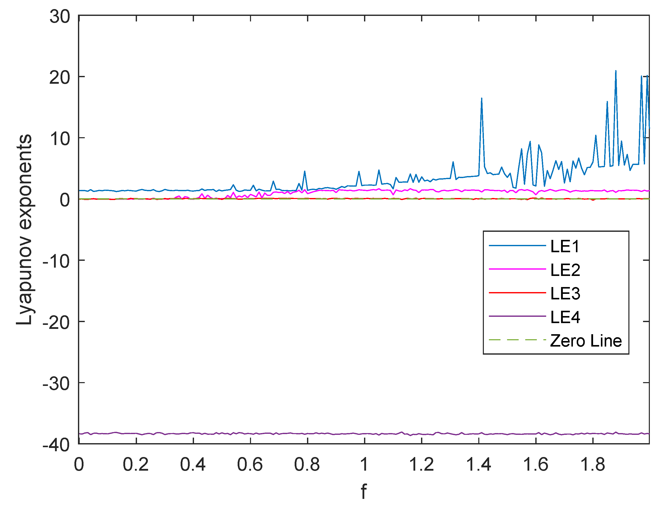
Figure 2.
Dynamics of Lyapunov exponents of the proposed 4D hyperchaotic system with the parameters , variable f from 0 to 2, and initial values .
Figure 2.
Dynamics of Lyapunov exponents of the proposed 4D hyperchaotic system with the parameters , variable f from 0 to 2, and initial values .
Figure 3.
Illustration of 2-bit and 3-bit permutation.
Figure 3.
Illustration of 2-bit and 3-bit permutation.
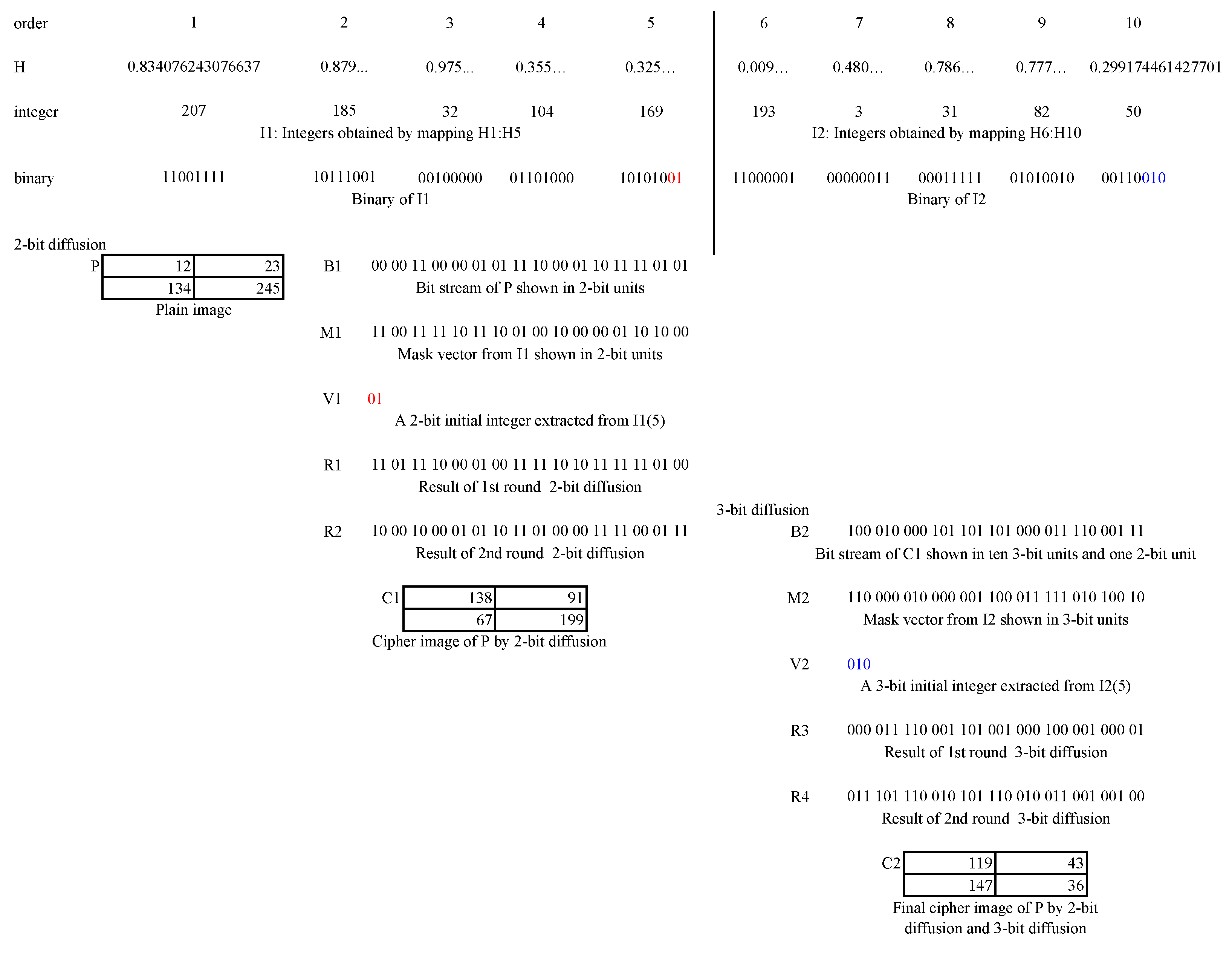
Figure 4.
Illustration of 2-bit and 3-bit diffusion.
Figure 4.
Illustration of 2-bit and 3-bit diffusion.
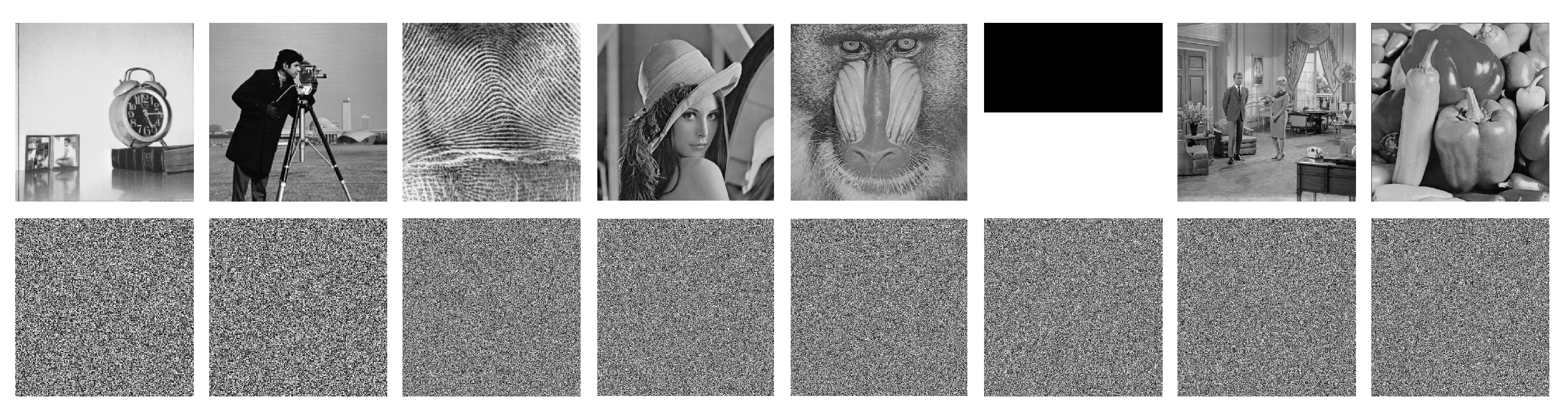
Figure 5.
Results of key sensitivity. The first row and the second row show the decrypted images by and , respectively. From left to right: Clock256, Cameraman256, Finger512, Lena512, Baboon512, Bw512, Couple512, and Peppers512.
Figure 5.
Results of key sensitivity. The first row and the second row show the decrypted images by and , respectively. From left to right: Clock256, Cameraman256, Finger512, Lena512, Baboon512, Bw512, Couple512, and Peppers512.
Figure 6.
Histograms of plain images and their corresponding cipher images. Each plain image is followed by its histogram, the corresponding cipher image, and its histogram.
Figure 6.
Histograms of plain images and their corresponding cipher images. Each plain image is followed by its histogram, the corresponding cipher image, and its histogram.
Figure 7.
Horizontal correlations of plain images and their corresponding cipher images.
Figure 7.
Horizontal correlations of plain images and their corresponding cipher images.
Figure 8.
Noise test. The first row, from left to right: cipher images with 0.5%, 1%, 2%, 4%, and 10% salt-and-pepper noise added. The second row: the decrypted images from the corresponding cipher images in the first row.
Figure 8.
Noise test. The first row, from left to right: cipher images with 0.5%, 1%, 2%, 4%, and 10% salt-and-pepper noise added. The second row: the decrypted images from the corresponding cipher images in the first row.
Figure 9.
Cropping test. The first row, from left to right: cipher images with 1%, 2.78%, 6.75%, 11.11%, and 25% data loss. The second row: the decrypted images from the corresponding cipher images in the first row.
Figure 9.
Cropping test. The first row, from left to right: cipher images with 1%, 2.78%, 6.75%, 11.11%, and 25% data loss. The second row: the decrypted images from the corresponding cipher images in the first row.
Table 1.
Experiment parameters.
Table 1.
Experiment parameters.
| Parameter Description | Value |
|---|
| Hyperchaotic system’s parameters | |
| Security keys | |
| Iteration number to generate discarded sequence | |
| Bit levels of permutation | |
| Bit levels of diffusion | |
| Rounds of encryption | 1 |
Table 2.
The SSIM values of decrypted images with and .
Table 2.
The SSIM values of decrypted images with and .
| Image Name | SSIM Value | Image Name | SSIM Value |
|---|
| Clock256 | 0.0083 | Cameraman256 | 0.0087 |
| Finger512 | 0.0081 | Lena512 | 0.0093 |
| Baboon512 | 0.0107 | Bw512 | 0.0047 |
| Couple512 | 0.0110 | Peppers512 | 0.0098 |
Table 3.
The SSIM values of cipher images with and .
Table 3.
The SSIM values of cipher images with and .
| Image Name | SSIM Value | Image Name | SSIM Value |
|---|
| Clock256 | 0.0011 | Cameraman256 | 0.0021 |
| Finger512 | 0.0052 | Lena512 | 0.0081 |
| Baboon512 | 0.0087 | Bw512 | 0.0060 |
| Couple512 | 0.0052 | Peppers512 | 0.0054 |
Table 4.
Information entropies of the testing images.
Table 4.
Information entropies of the testing images.
| Image Name | Plain Image | Cipher Image |
|---|
| MBPD | DFDLC [13] | HCDNA [38] | CDCP [47] |
|---|
| Airplane256 | 6.4523 | 7.9970 | 7.9974 | 7.9961 | 7.9975 |
| Clock256 | 6.7057 | 7.9970 | 7.9974 | 7.9957 | 7.9972 |
| Cameraman256 | 7.0492 | 7.9976 | 7.9972 | 7.9961 | 7.9975 |
| Cameraman512 | 7.0480 | 7.9994 | 7.9992 | 7.9982 | 7.9993 |
| Finger512 | 6.7279 | 7.9994 | 7.9993 | 7.9991 | 7.9993 |
| Gray512 | 4.3923 | 7.9992 | 7.9993 | 7.9920 | 7.9993 |
| Lena512 | 7.4460 | 7.9993 | 7.9994 | 7.9989 | 7.9993 |
| Baboon512 | 7.1391 | 7.9994 | 7.9994 | 7.9993 | 7.9993 |
| Barbara512 | 7.6321 | 7.9993 | 7.9994 | 7.9993 | 7.9993 |
| Boat512 | 7.1914 | 7.9992 | 7.9994 | 7.9990 | 7.9993 |
| Bw512 | 1.0000 | 7.9992 | 7.9992 | 7.9154 | 7.9993 |
| Couple512 | 7.0572 | 7.9993 | 7.9993 | 7.9992 | 7.9994 |
| Houses512 | 7.6548 | 7.9993 | 7.9993 | 7.9993 | 7.9992 |
| Peppers512 | 7.5925 | 7.9994 | 7.9994 | 7.9992 | 7.9994 |
| Pirate512 | 7.2367 | 7.9993 | 7.9993 | 7.9990 | 7.9993 |
| Truck512 | 6.0274 | 7.9994 | 7.9994 | 7.9991 | 7.9993 |
Table 5.
The correlation coefficients of the testing images.
Table 5.
The correlation coefficients of the testing images.
| Image Name | | Plain Image | Cipher Image |
|---|
| MBPD | DFDLC [13] | HCDNA [38] | CDCP [47] |
|---|
| Airplane256 | | 0.9562 | −0.0062 | 0.0004 | −0.0049 | −0.0003 |
| 0.8742 | 0.0006 | −0.0042 | −0.0045 | −0.0006 |
| 0.8995 | 0.0019 | 0.0001 | 0.0038 | −0.0022 |
| Clock256 | | 0.9540 | −0.0024 | 0.0034 | 0.0017 | 0.0020 |
| 0.9734 | −0.0107 | 0.0022 | −0.0060 | −0.0017 |
| 0.9376 | 0.0013 | 0.0026 | −0.0015 | −0.0031 |
| Cameraman256 | | 0.9554 | −0.0059 | 0.0015 | −0.0006 | −0.0013 |
| 0.9710 | 0.0007 | 0.0023 | −0.0012 | 0.0001 |
| 0.9377 | 0.0052 | −0.0053 | 0.0012 | −0.0030 |
| Cameraman512 | | 0.9830 | −0.0013 | −0.0016 | −0.0014 | 0.0011 |
| 0.9887 | 0.0014 | 0.0015 | 0.0029 | −0.0026 |
| 0.9746 | −0.0017 | 0.0002 | −0.0022 | 0.0010 |
| Finger512 | | 0.9343 | 0.0022 | −0.0010 | −0.0012 | −0.0002 |
| 0.9168 | 0.0007 | −0.0012 | −0.0005 | −0.0005 |
| 0.8664 | 0.0017 | 0.0001 | −0.0003 | −0.0003 |
| Gray512 | | 0.9913 | 0.0028 | −0.0006 | 0.0017 | 0.0001 |
| 0.9989 | 0.0009 | 0.0021 | −0.0010 | 0.0017 |
| 0.9964 | 0.0005 | −0.0006 | −0.0007 | 0.0007 |
| Lena512 | | 0.9705 | 0.0005 | 0.0014 | 0.0022 | −0.0028 |
| 0.9856 | 0.0002 | −0.0004 | −0.0004 | 0.0038 |
| 0.9649 | 0.0000 | 0.0021 | −0.0008 | 0.0023 |
| Baboon512 | | 0.8652 | −0.0018 | 0.0024 | 0.0020 | −0.0024 |
| 0.7524 | −0.0017 | −0.0000 | 0.0027 | 0.0024 |
| 0.7210 | 0.0022 | 0.0026 | 0.0011 | 0.0012 |
| Barbara512 | | 0.8940 | 0.0000 | 0.0001 | 0.0007 | −0.0001 |
| 0.9572 | 0.0002 | 0.0034 | −0.0018 | −0.0001 |
| 0.8942 | 0.0004 | −0.0006 | −0.0001 | −0.0014 |
| Boat512 | | 0.9368 | 0.0022 | −0.0015 | −0.0022 | −0.0052 |
| 0.9709 | 0.0007 | 0.0008 | −0.0004 | 0.0025 |
| 0.9240 | −0.0007 | 0.0012 | 0.0015 | 0.0021 |
| Bw512 | | 1.0000 | −0.0013 | −0.0009 | −0.0001 | −0.0022 |
| 0.9922 | 0.0031 | 0.0050 | −0.0016 | −0.0019 |
| 0.9961 | −0.0011 | −0.0019 | 0.0002 | −0.0008 |
| Couple512 | | 0.9451 | 0.0013 | 0.0020 | 0.0007 | 0.0019 |
| 0.9514 | 0.0011 | 0.0002 | 0.0020 | 0.0032 |
| 0.9116 | −0.0015 | −0.0011 | −0.0006 | 0.0001 |
| Houses512 | | 0.9077 | −0.0013 | 0.0028 | 0.0014 | −0.0030 |
| 0.9173 | −0.0002 | 0.0000 | −0.0026 | 0.0016 |
| 0.8439 | 0.0014 | 0.0005 | 0.0010 | −0.0011 |
| Peppers512 | | 0.9733 | −0.0009 | 0.0006 | −0.0004 | 0.0001 |
| 0.9763 | −0.0021 | −0.0024 | 0.0007 | −0.0006 |
| 0.9650 | 0.0005 | 0.0007 | 0.0011 | −0.0008 |
| Pirate512 | | 0.9593 | −0.0006 | 0.0014 | −0.0020 | −0.0020 |
| 0.9675 | −0.0022 | 0.0006 | −0.0008 | 0.0006 |
| 0.9432 | 0.0002 | −0.0010 | −0.0003 | −0.0023 |
| Truck512 | | 0.9610 | 0.0005 | 0.0000 | 0.0012 | 0.0035 |
| 0.9164 | 0.0018 | 0.0001 | 0.0003 | −0.0004 |
| 0.9048 | −0.0028 | −0.0003 | −0.0016 | −0.0005 |
Table 6.
The average NPCR (%) of running the schemes 20 times.
Table 6.
The average NPCR (%) of running the schemes 20 times.
| Image | MBPD | DFDLC [13] | HCDNA [38] | CDCP [47] |
|---|
| Airplane256 | 99.6014
% | 99.6125% | 76.4828% | 99.6374% |
| Clock256 | 99.6114% | 99.6085% | 65.7269% | 99.7081% |
| Cameraman256 | 99.6099% | 99.6196% | 73.4785% | 99.7564% |
| Cameraman512 | 99.6112% | 99.6078% | 67.1009% | 99.6590% |
| Finger512 | 99.6083% | 99.6108% | 76.2949% | 99.6928% |
| Gray512 | 99.6088% | 99.6131% | 61.1288% | 99.6767% |
| Lena512 | 99.6062% | 99.6084% | 66.5552% | 99.6849% |
| Baboon512 | 99.6104% | 99.6077% | 64.3461% | 99.6372% |
| Barbara512 | 99.6113% | 99.6114% | 73.5446% | 99.5927% |
| Boat512 | 99.6093% | 99.6089% | 75.0493% | 99.4786% |
| Bw512 | 99.5997% | 89.6501% | 64.8879% | 99.7000% |
| Couple512 | 99.6033% | 99.6045% | 63.5847% | 99.7910% |
| Houses512 | 99.6037% | 99.6092% | 75.8256% | 99.7578% |
| Peppers512 | 99.6090% | 99.6100% | 73.8790% | 99.6849% |
| Pirate512 | 99.6082% | 99.6087% | 73.9838% | 99.6765% |
| Truck512 | 99.6063% | 99.6070% | 66.5778% | 99.7033% |
| Pass/Fail/All | 16/0/16 | 15/1/16 | 0/16/16 | 15/1/16 |
| Std. | 0.0037% | 2.4899% | 5.3211% | 0.0723% |
| Mean | 99.6074% | 98.9874% | 69.9029% | 99.6773% |
Table 7.
The average UACI (%) of running the schemes 20 times.
Table 7.
The average UACI (%) of running the schemes 20 times.
| Image | MBPD | DFDLC [13] | HCDNA [38] | CDCP [47] |
|---|
| Airplane256 | 33.4400
% | 33.4256% | 30.6926% | 33.4682% |
| Clock256 | 33.4610% | 33.4992% | 28.3912% | 33.5090% |
| Cameraman256 | 33.4312% | 33.4529% | 31.3096% | 33.4766% |
| Cameraman512 | 33.4618% | 33.4547% | 27.7148% | 33.4765% |
| Finger512 | 33.4552% | 33.4766% | 33.6617% | 33.4796% |
| Gray512 | 33.4628% | 33.4638% | 25.1829% | 33.4842% |
| Lena512 | 33.4545% | 33.4581% | 27.2038% | 33.4484% |
| Baboon512 | 33.4590% | 33.4528% | 26.1169% | 33.4996% |
| Barbara512 | 33.4905% | 33.4746% | 28.2405% | 33.5072% |
| Boat512 | 33.4684% | 33.4781% | 31.6422% | 33.4881% |
| Bw512 | 33.4899% | 30.1296% | 22.3338% | 33.4655% |
| Couple512 | 33.4661% | 33.4853% | 25.9647% | 33.4975% |
| Houses512 | 33.4682% | 33.4631% | 31.4138% | 33.4587% |
| Peppers512 | 33.4409% | 33.4255% | 29.2497% | 33.4637% |
| Pirate512 | 33.4808% | 33.4251% | 30.3032% | 33.5917% |
| Truck512 | 33.4612% | 33.4609% | 28.0393% | 33.4589% |
| Pass/Fail/All | 16/0/16 | 15/1/16 | 0/16/16 | 15/1/16 |
| Std. | 0.0164% | 0.8328% | 2.8880% | 0.0335% |
| Mean | 33.4620% | 33.2516% | 28.5913% | 33.4858% |
Table 8.
Running time of encryption and decryption (in seconds).
Table 8.
Running time of encryption and decryption (in seconds).
| Operation | Size | MBPD | DFDLC [13] | HCDNA [38] | CDCP [47] |
|---|
| Encryption | | 0.8158 | 0.8479 | 3.4635 | 0.1268 |
| 3.3833 | 3.4261 | 14.2808 | 0.5240 |
| Decryption | | 0.8136 | 0.8366 | 4.7181 | 0.1305 |
| 3.3624 | 3.4116 | 19.5680 | 0.5126 |
Table 9.
Results obtained by the proposed MBPD on miscellaneous images from the SIPI image database.
Table 9.
Results obtained by the proposed MBPD on miscellaneous images from the SIPI image database.
| Image | Size | Entropy | | | | NPCR | UACI |
|---|
| 5.1.10 | | 7.9973 | 0.0010 | −0.0024 | −0.0003 | 99.6053% | 33.4448% |
| 5.1.13 | | 7.9976 | 0.0011 | 0.0000 | −0.0016 | 99.6127% | 33.4409% |
| 5.1.14 | | 7.9974 | −0.0022 | 0.0000 | −0.0010 | 99.6114% | 33.5188% |
| Moonsurface256 | | 7.9973 | 0.0023 | −0.0042 | −0.0012 | 99.6093% | 33.4342% |
| 5.2.10 | | 7.9992 | 0.0010 | −0.0040 | 0.0005 | 99.6116% | 33.4516% |
| 7.1.02 | | 7.9993 | −0.0007 | 0.0018 | −0.0004 | 99.6083% | 33.4698% |
| 7.1.03 | | 7.9993 | −0.0040 | 0.0017 | −0.0004 | 99.6070% | 33.4621% |
| 7.1.04 | | 7.9993 | 0.0001 | −0.0006 | −0.0027 | 99.6060% | 33.4578% |
| 7.1.05 | | 7.9993 | −0.0017 | −0.0027 | 0.0013 | 99.6114% | 33.4616% |
| 7.1.06 | | 7.9994 | 0.0028 | 0.0015 | −0.0027 | 99.6074% | 33.4786% |
| 7.1.07 | | 7.9993 | 0.0018 | −0.0006 | −0.0004 | 99.6066% | 33.4736% |
| 7.1.08 | | 7.9994 | 0.0007 | −0.0012 | −0.0000 | 99.6093% | 33.4505% |
| 7.1.09 | | 7.9993 | 0.0003 | −0.0035 | 0.0011 | 99.6142% | 33.4582% |
| 7.1.10 | | 7.9992 | −0.0026 | −0.0007 | −0.0000 | 99.6109% | 33.4435% |
| Aerial512 | | 7.9993 | 0.0002 | −0.0016 | 0.0004 | 99.6075% | 33.4789% |
| ruler.512 | | 7.9993 | −0.0045 | −0.0001 | −0.0010 | 99.6134% | 33.4642% |
| 5.3.01 | | 7.9998 | −0.0006 | −0.0017 | 0.0002 | 99.6117% | 33.4545% |
| 5.3.02 | | 7.9998 | 0.0014 | 0.0000 | 0.0004 | 99.6090% | 33.4637% |
| 7.2.01 | | 7.9998 | 0.0005 | −0.0001 | −0.0006 | 99.6127% | 33.4609% |
| 4.1.01 | | 7.9969 | 0.0016 | 0.0031 | 0.0027 | 99.6155% | 33.4652% |
| 4.1.02 | | 7.9975 | −0.0068 | −0.0037 | 0.0032 | 99.6149% | 33.4376% |
| 4.1.03 | | 7.9971 | 0.0029 | −0.0029 | −0.0001 | 99.6168% | 33.4728% |
| 4.1.04 | | 7.9972 | 0.0013 | 0.0024 | 0.0001 | 99.5991% | 33.4596% |
| 4.1.05 | | 7.9974 | 0.0030 | 0.0031 | −0.0008 | 99.6046% | 33.4304% |
| 4.1.06 | | 7.9971 | −0.0030 | 0.0009 | 0.0020 | 99.6051% | 33.3983% |
| 4.1.07 | | 7.9972 | 0.0002 | −0.0003 | −0.0049 | 99.6139% | 33.4285% |
| 4.1.08 | | 7.9970 | 0.0024 | −0.0008 | 0.0003 | 99.6086% | 33.4542% |
| 4.2.01 | | 7.9993 | 0.0014 | −0.0005 | −0.0006 | 99.6051% | 33.4530% |
| 4.2.03 | | 7.9992 | −0.0011 | 0.0032 | 0.0017 | 99.6102% | 33.4833% |
| 4.2.05 | | 7.9994 | −0.0004 | −0.0002 | −0.0004 | 99.6111% | 33.4447% |
| 4.2.06 | | 7.9993 | 0.0004 | −0.0016 | −0.0006 | 99.6106% | 33.4843% |
| 4.2.07 | | 7.9993 | −0.0013 | −0.0001 | −0.0000 | 99.6087% | 33.4446% |
| house | | 7.9992 | −0.0012 | 0.0005 | −0.0010 | 99.6079% | 33.4962% |


