
Numerical Simulation Study on Flow Laws and Heat Transfer of Gas Hydrate in the Spiral Flow Pipeline with Long Twisted Band


Abstract
1. Introduction
2. Numerical Simulation Method
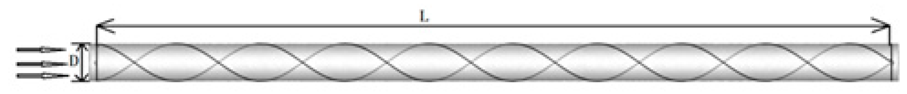
2.1. Physical Model
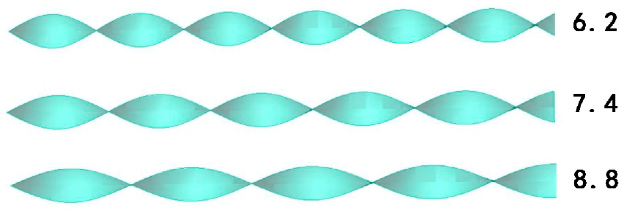
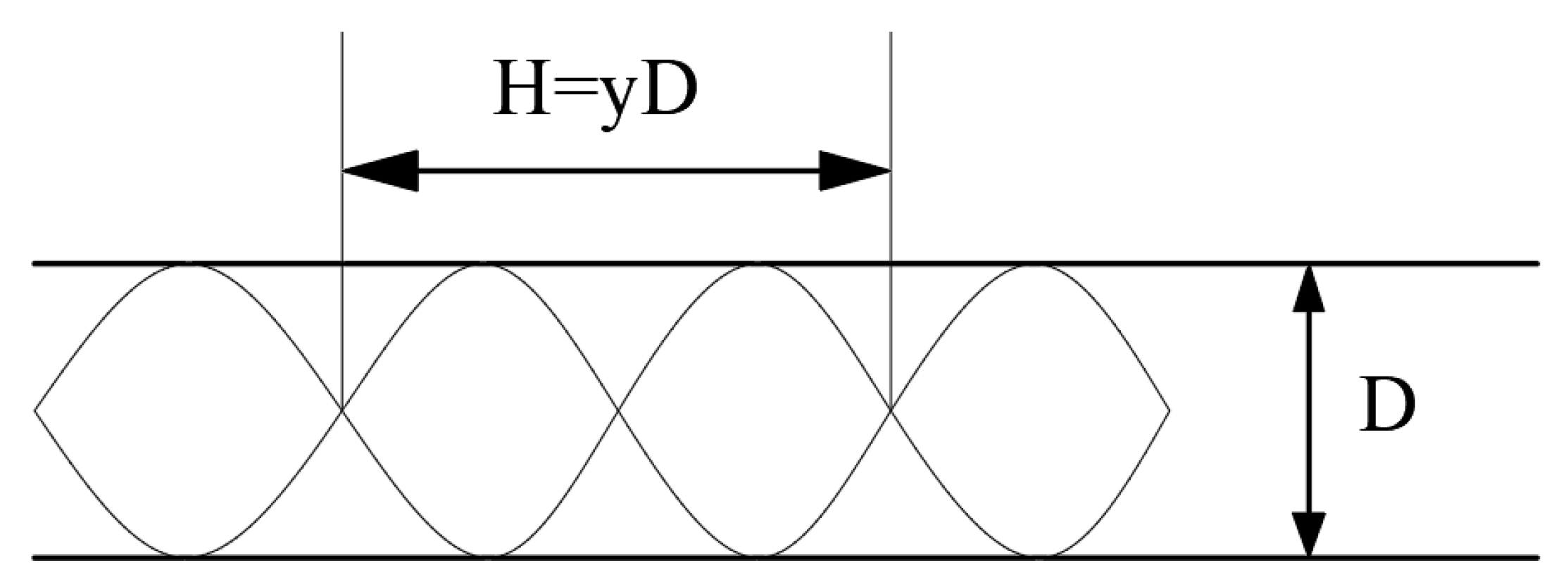
2.1.1. Geometric Model
2.1.2. Boundary Conditions
2.1.3. Initial Conditions
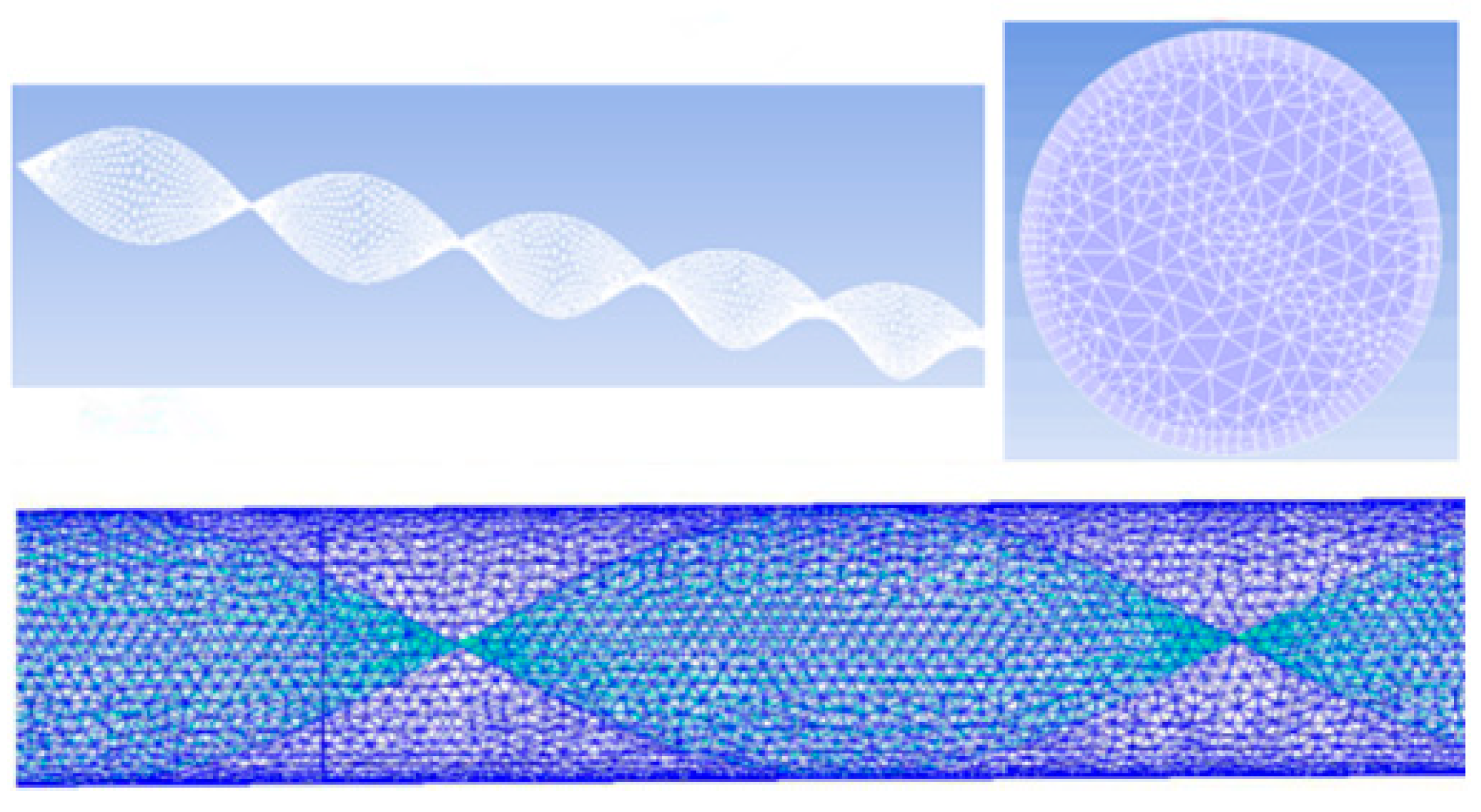
2.2. Meshing
2.3. Mathematical Model
2.3.1. Governing Equations
2.3.2. Turbulent Motion Equation
2.3.3. Discrete Phase Model
2.4. Calculation Method
2.5. Numerical Examples Validate
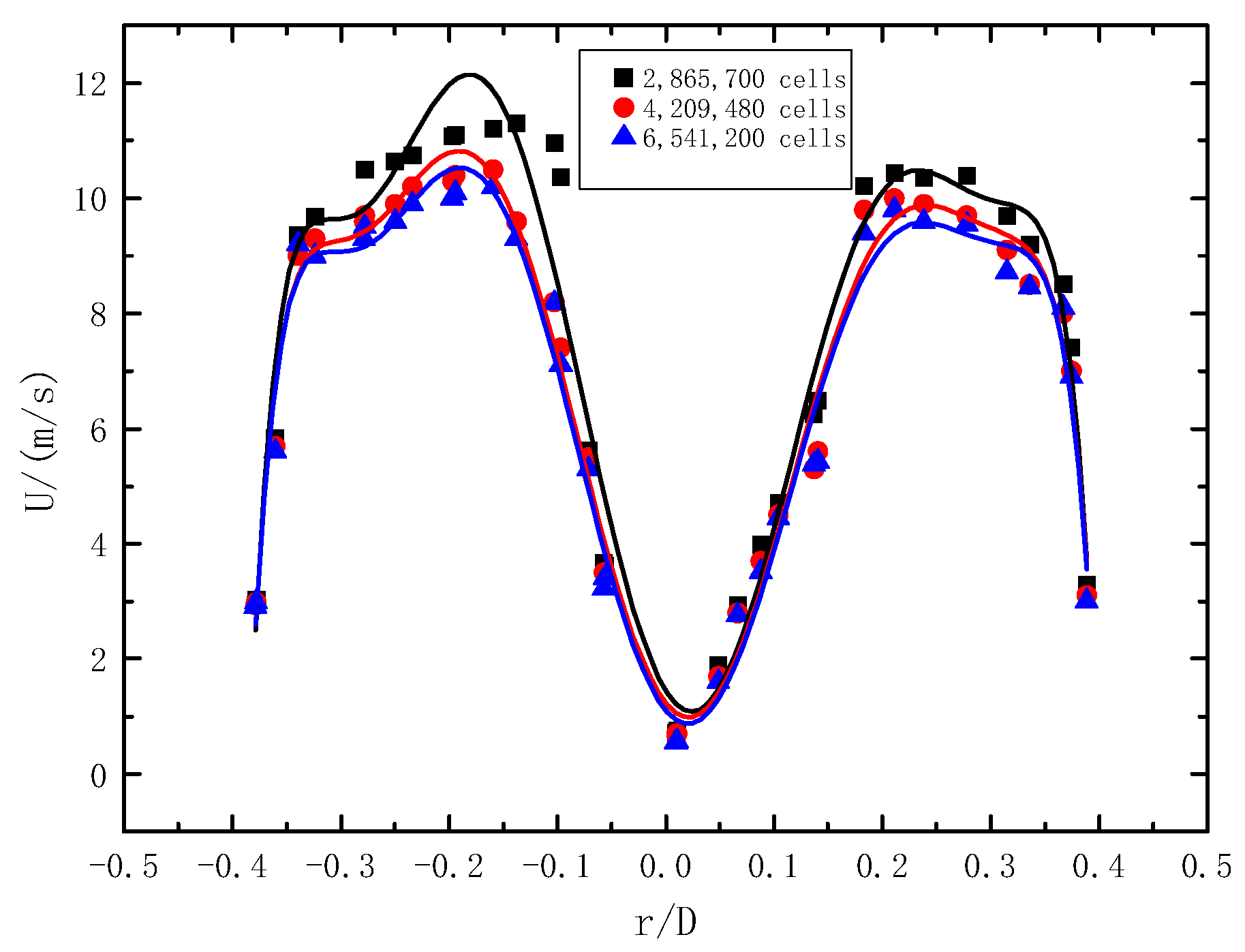
2.5.1. Grid Independence Test
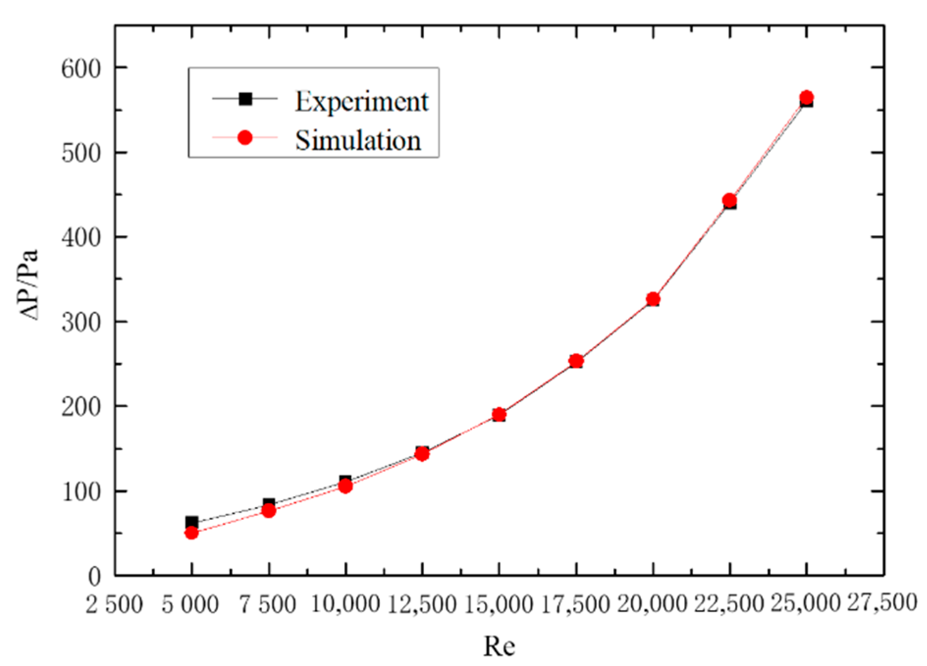
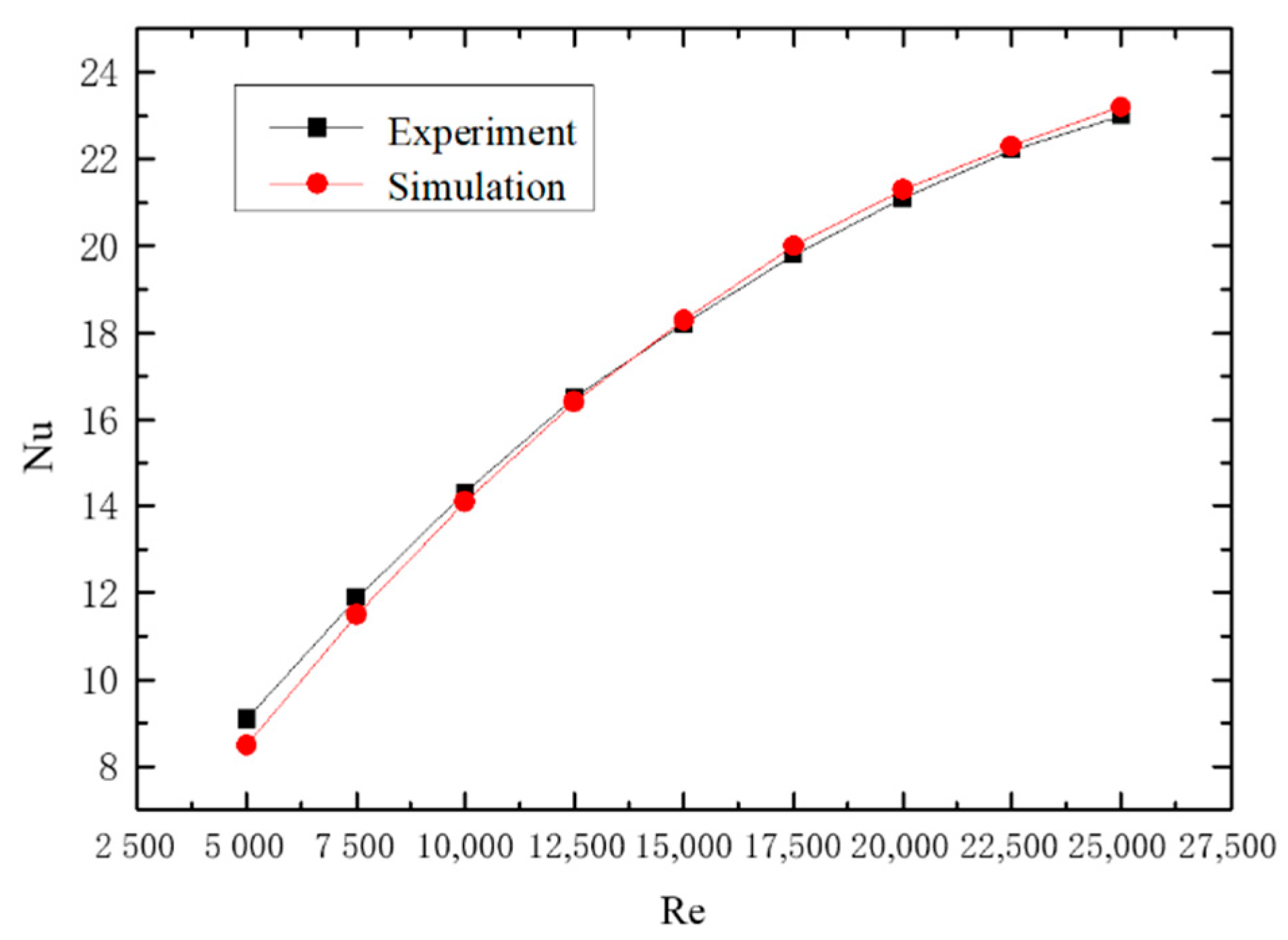
2.5.2. Experimental Verification of Gas–Solid Two-Phase Spiral Flow and Heat Transfer
3. Results
3.1. Velocity Distribution Law
3.2. Distribution Law of Spiral Flow Pressure Drop
3.2.1. Influence of Reynolds Number on Pressure Drop
3.2.2. Influence of Twisted Rate on Pressure Drop
3.3. Analysis of Heat Transfer Law
3.3.1. Axial Temperature Distribution Law
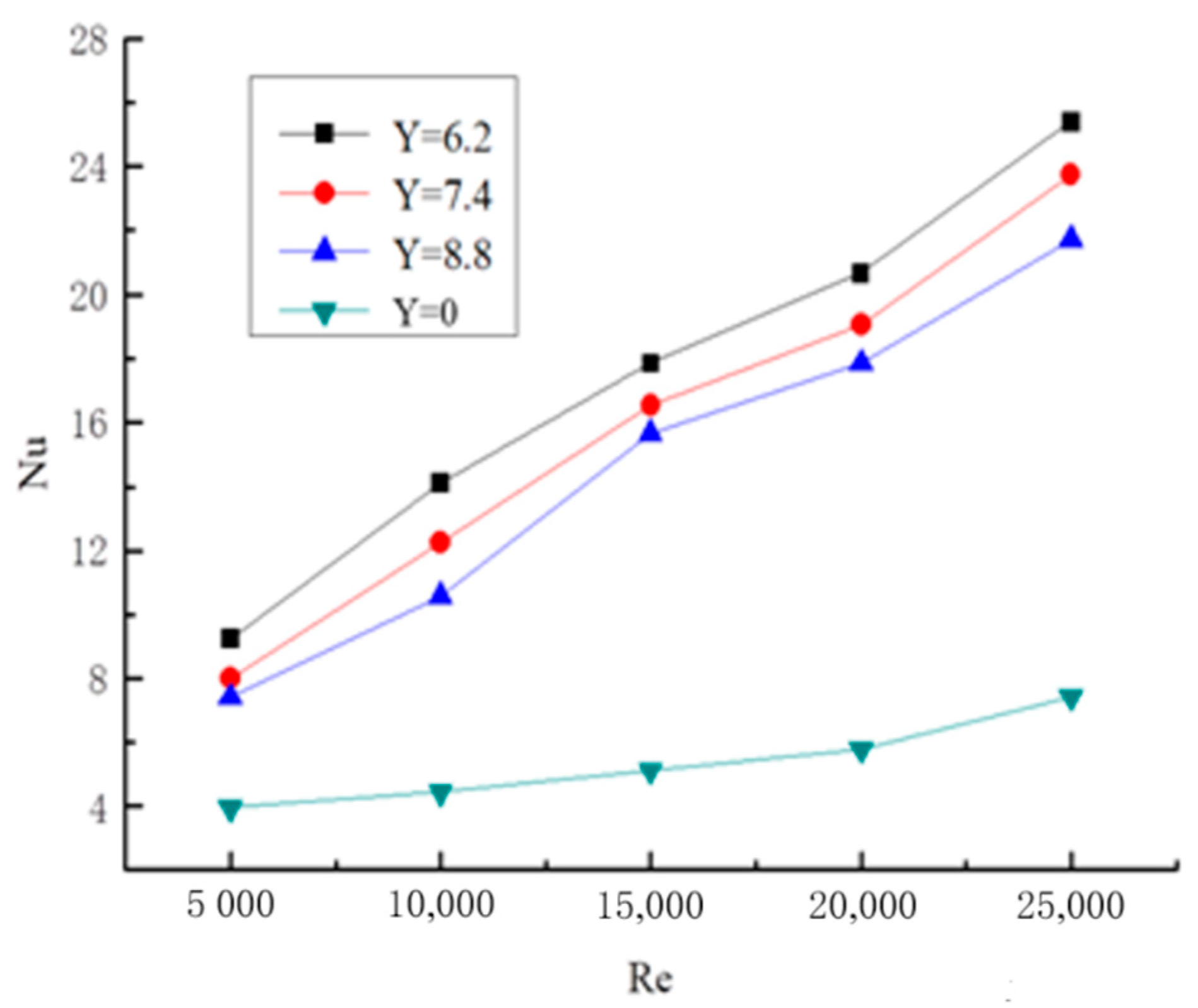
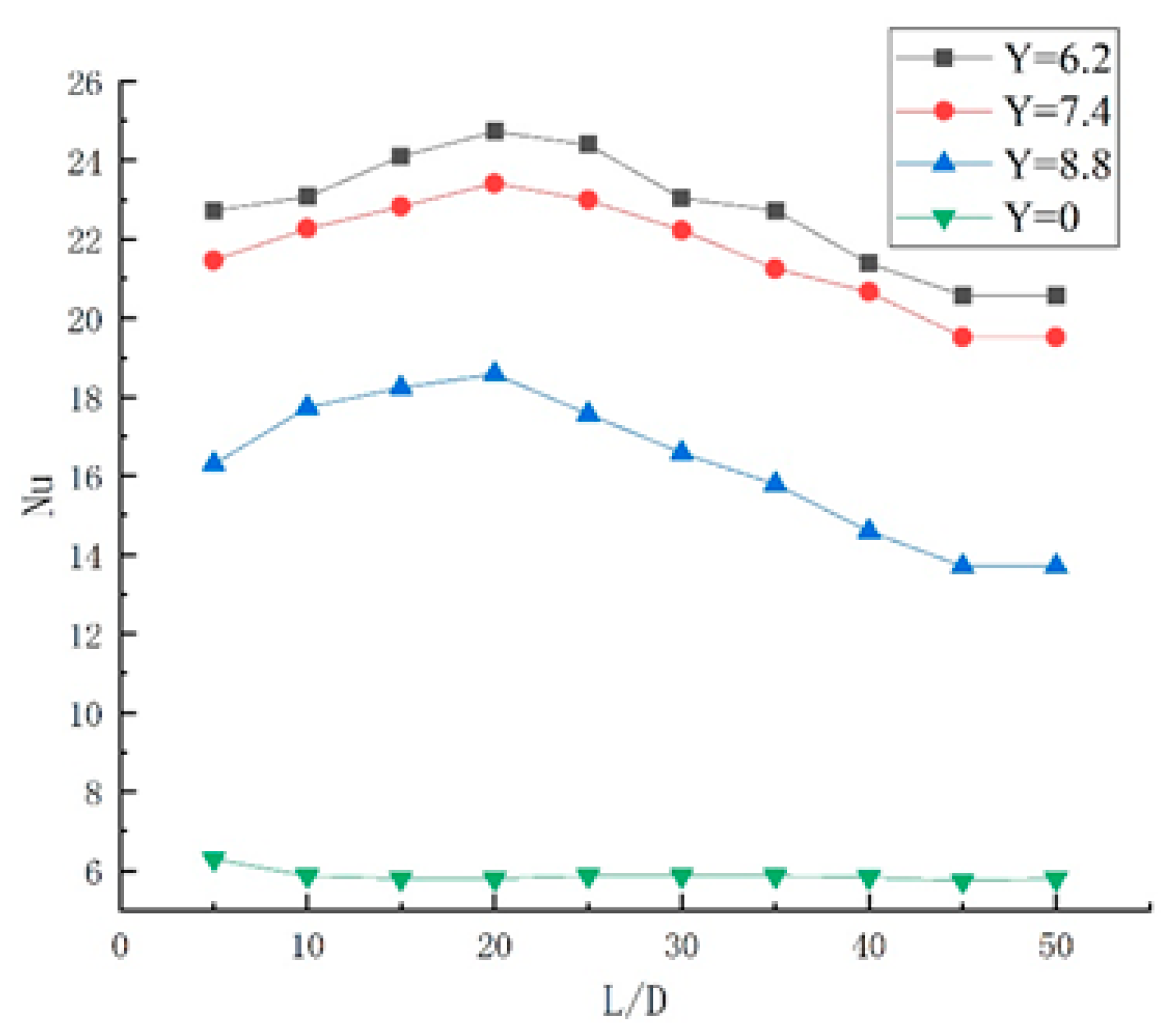
3.3.2. Axial Distribution Law of Nusselt Number
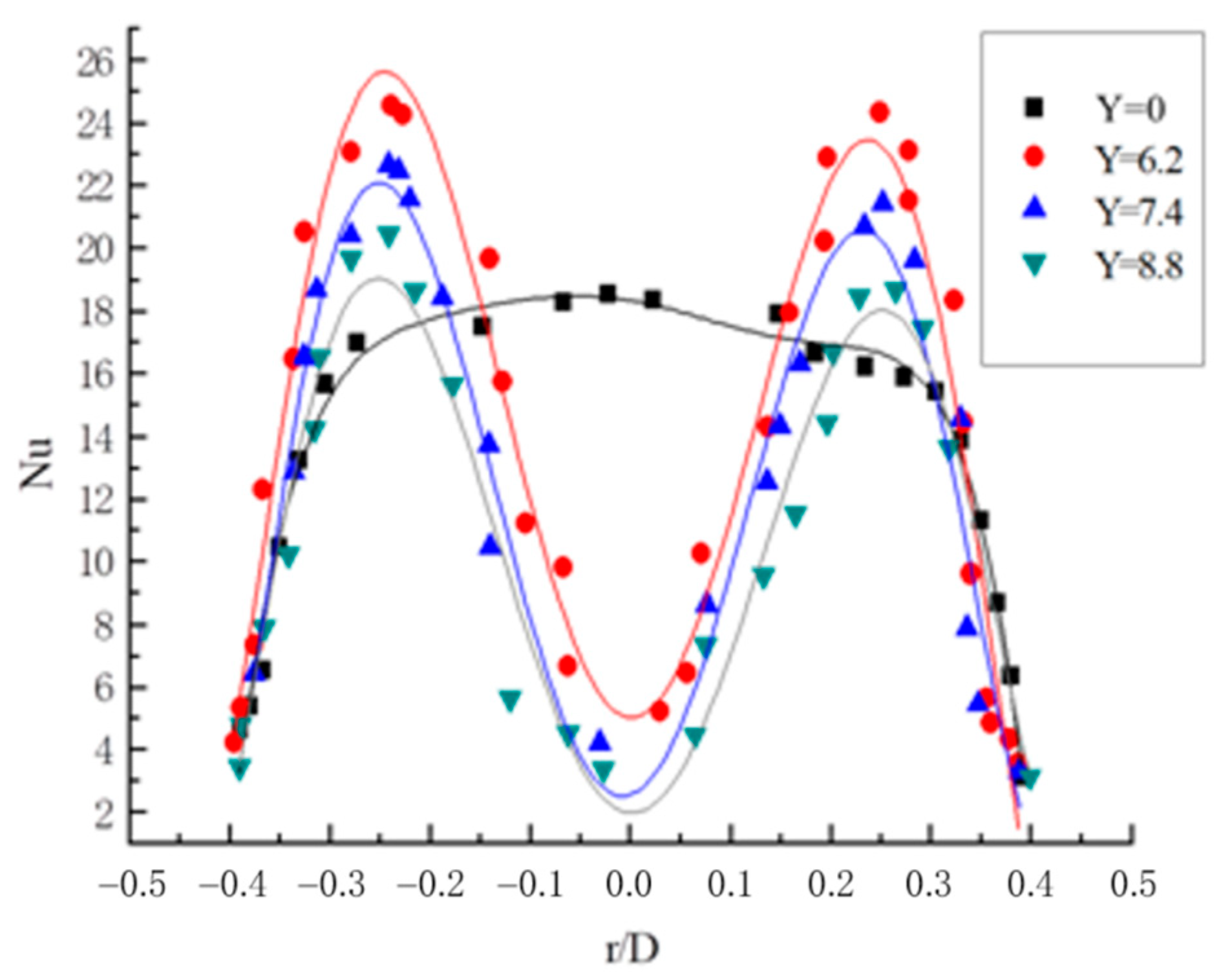
3.3.3. Radial Distribution Law of Nusselt Number
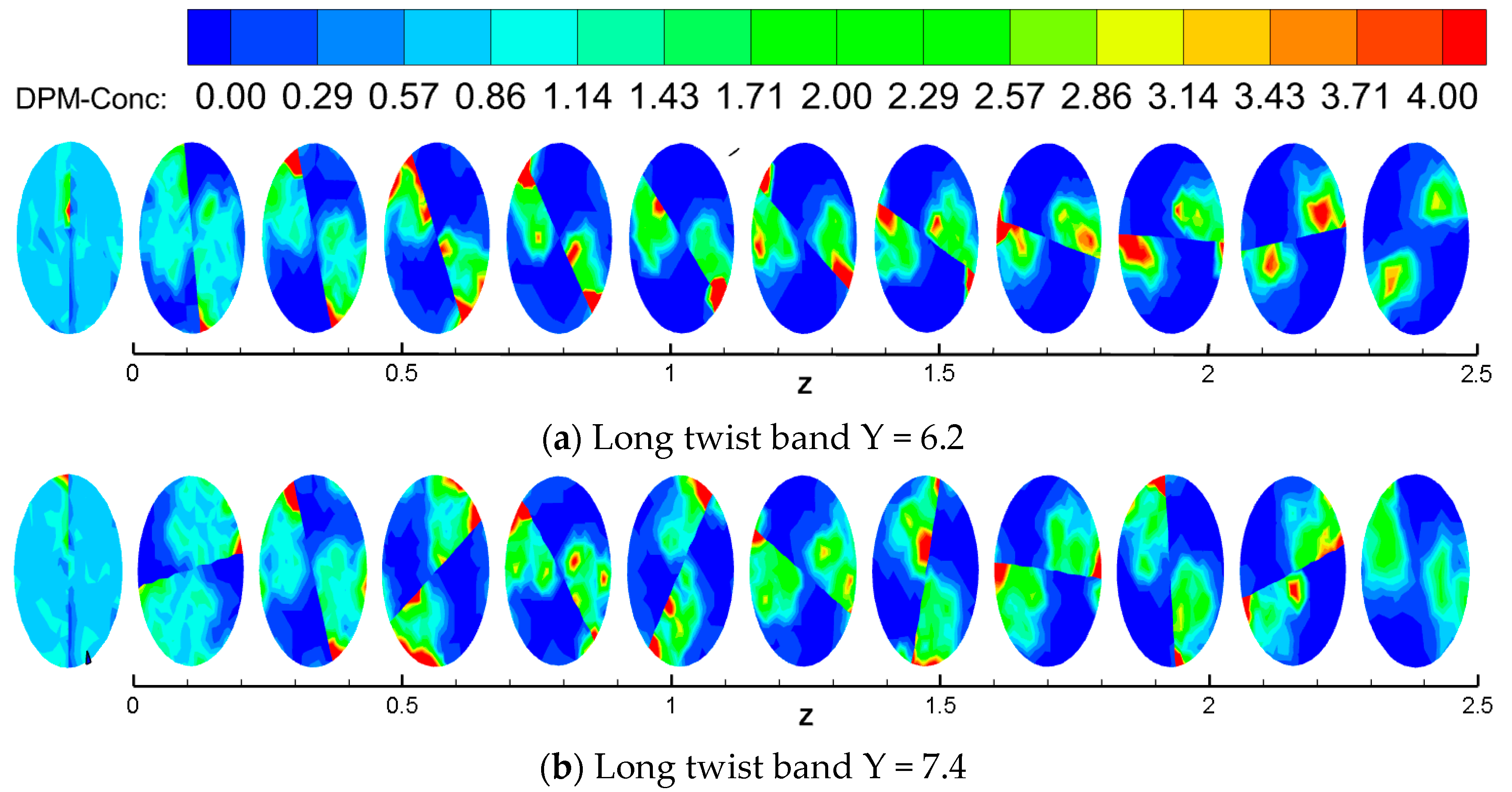
3.4. Particle Deposition Law
4. Conclusions
- (1)
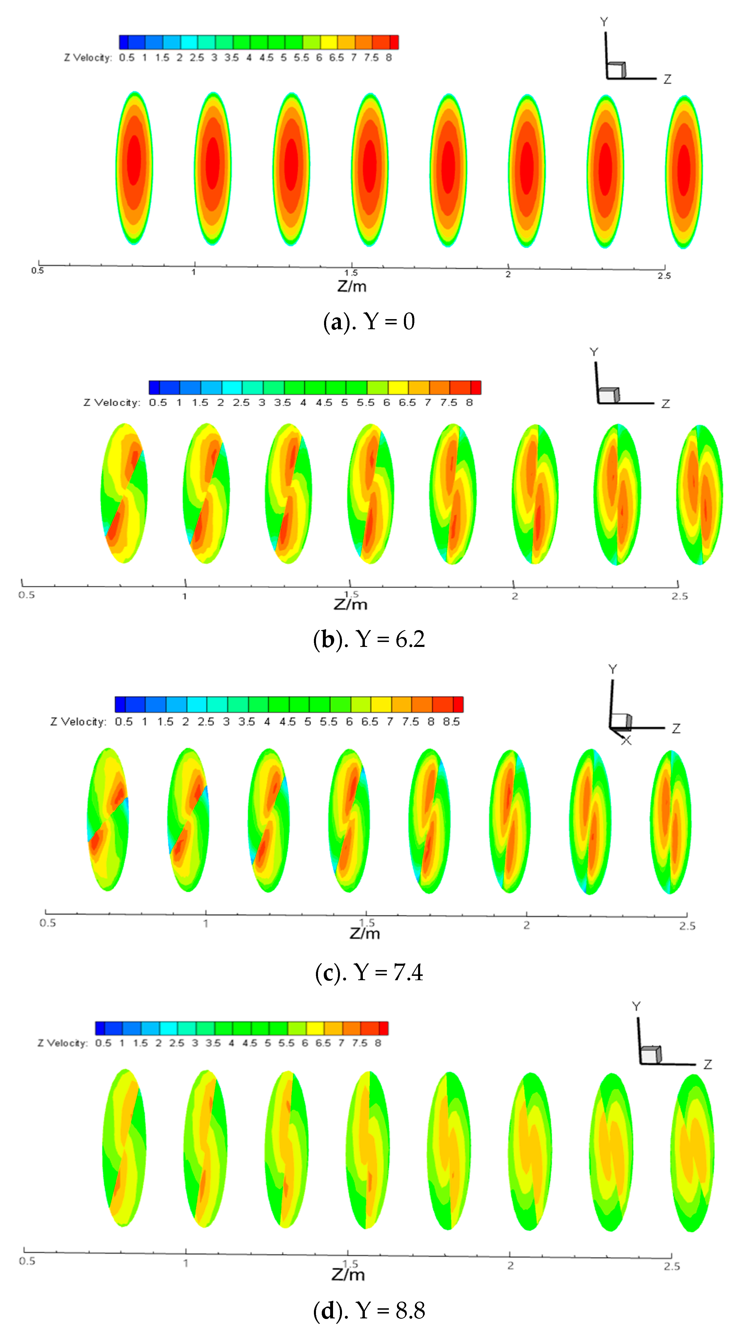
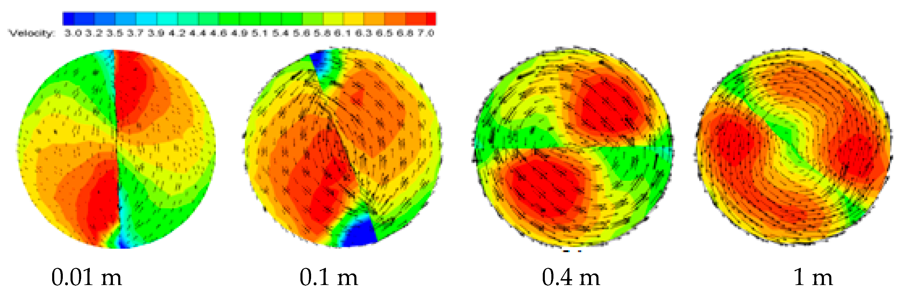
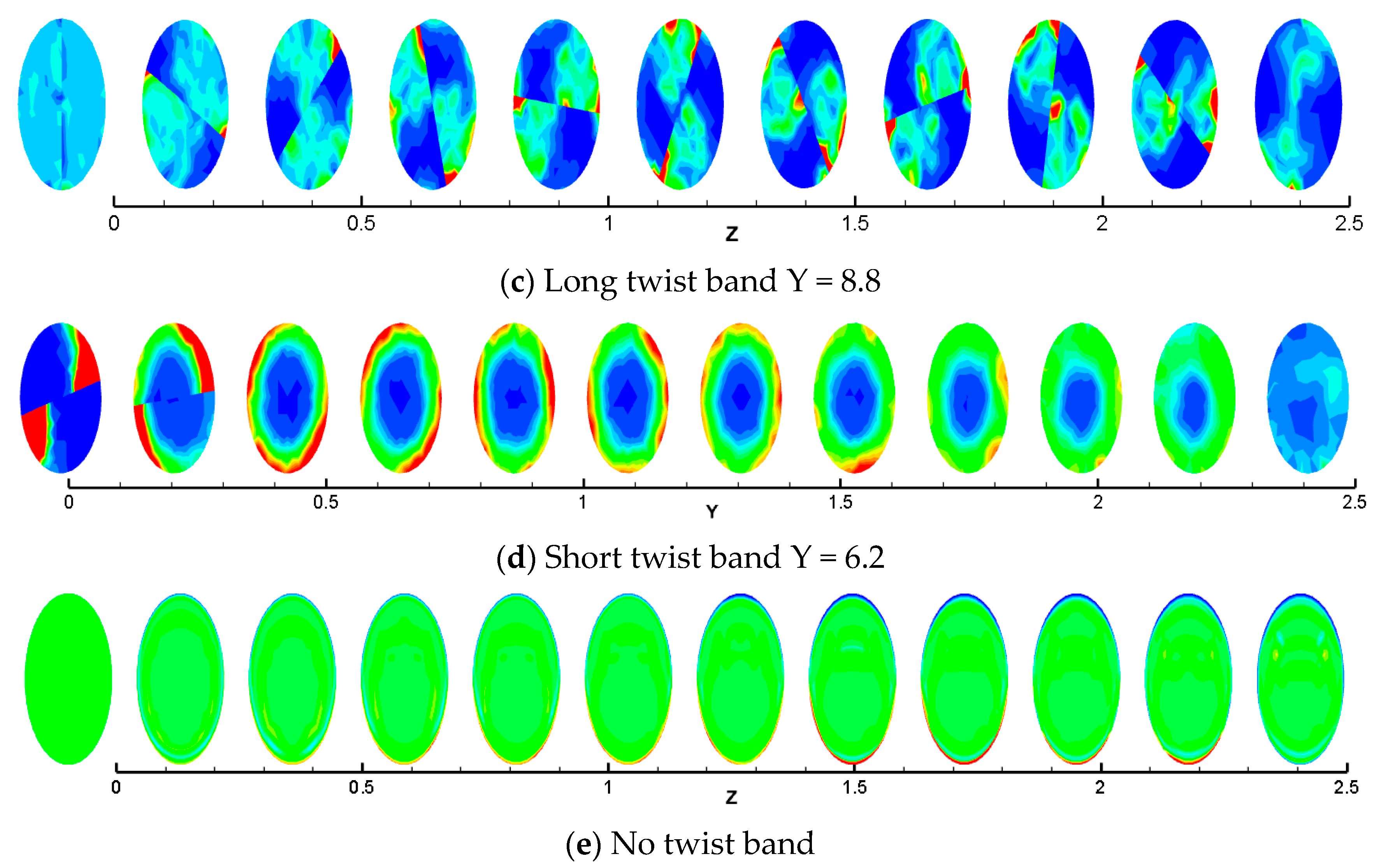
- In the plain direct current of a light pipe without a twisted band, the velocity is maximum in the central area of the pipe and then decreases uniformly toward the pipe wall, and the velocity change at each section is not obvious. However, two distinct eddies are formed on both sides of the twisted band with the maximum velocity at the center of the vortex. Along the direction of the pipe, the two vortices move from the near twisted band toward the wall, and it can effectively carry the hydrate particles deposited on the pipe wall.
- (2)
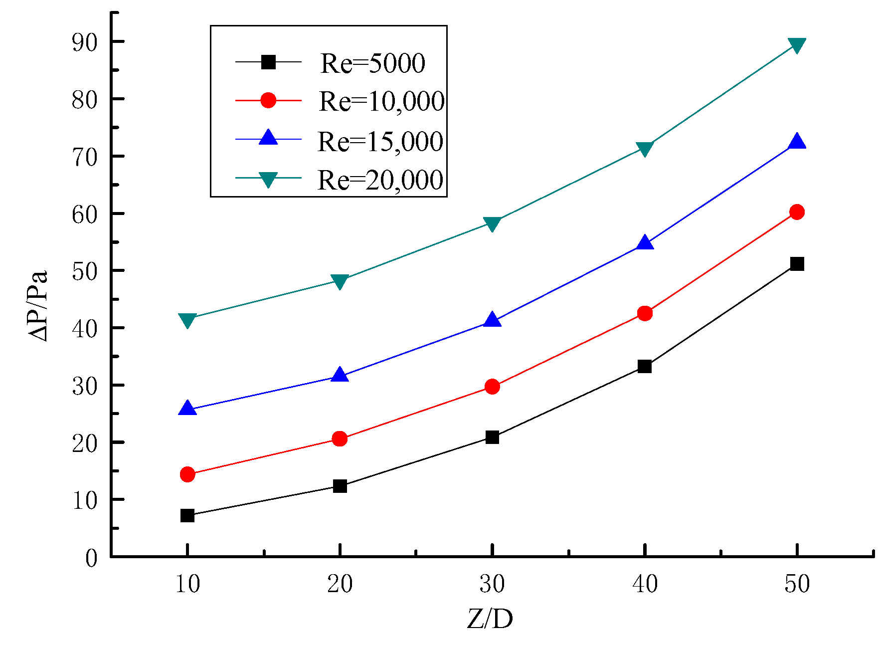
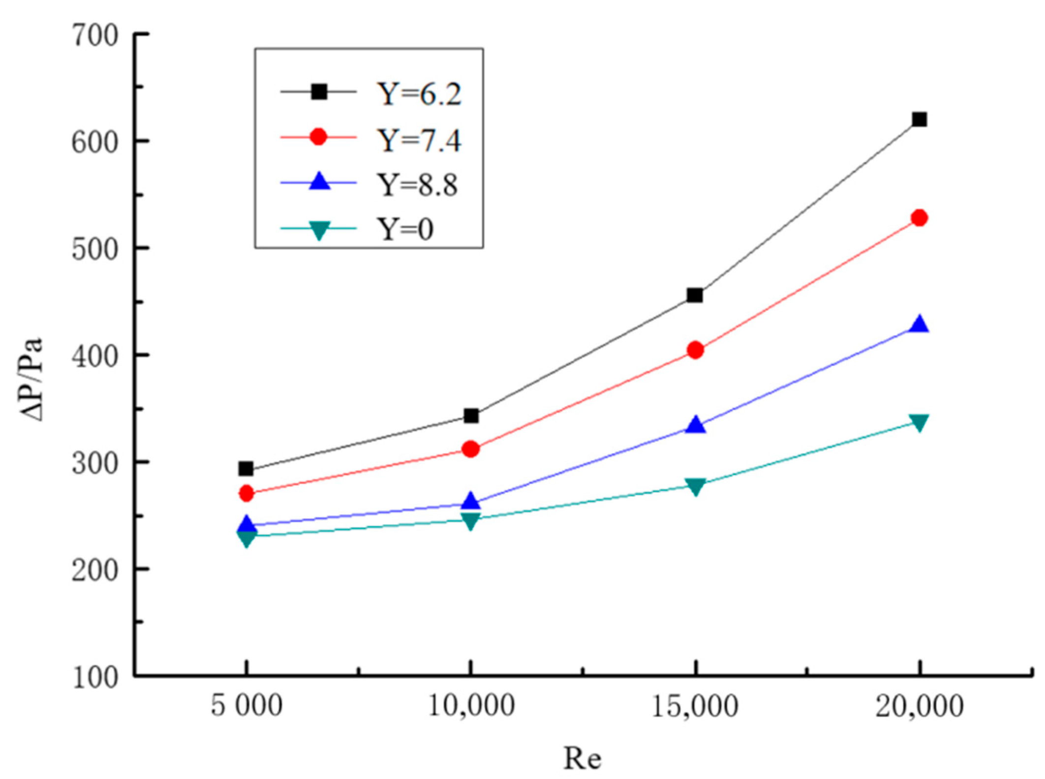
- At the same section of the pipe, the pressure drop of the pipe increases with the increase of Reynolds number; when the Reynolds number is higher, there are greater increases of pressure drop. Along the direction of the pipeline, the pressure drop becomes more obvious with the increase of particle transport distance, and the pressure drop curve is similar to a parabola. In the case of constant particle Reynolds number, the twisted rate is greater, the spiral flow strength is weaker, the tangential velocity is smaller, the axial velocity loss is smaller, and the pressure drop is smaller. Therefore, the pressure loss can be reduced as much as possible while the effect of spiral flow can be guaranteed.
- (3)
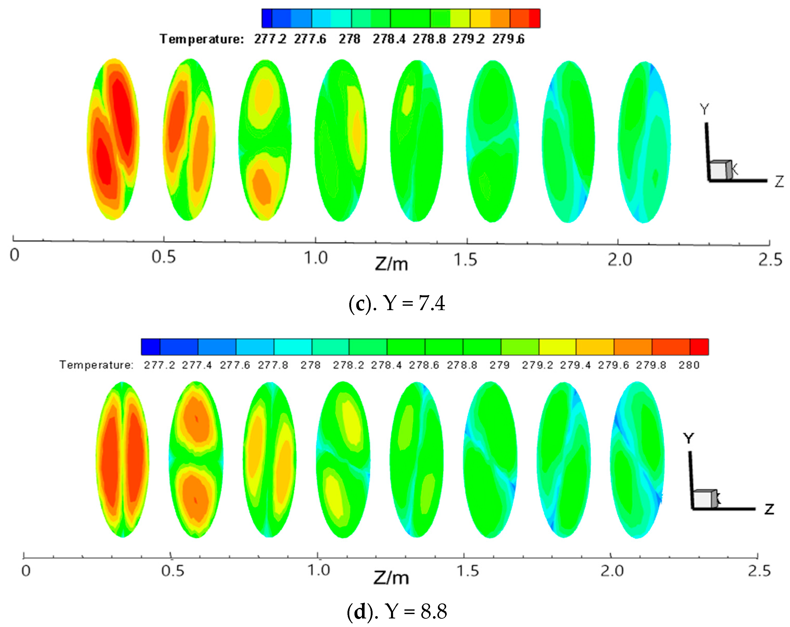
- In a straight light pipe flow without a twisted band, the Nusselt number is in a parabolic shape with the opening downwards. At the center of the pipe, the Nusselt number gradually decreases toward the pipe wall at the maximum, and the attenuation gradient of Nu is large at the near wall. The curve of Nusselt number appears as a trough in the center of the pipe and a peak at half of the pipe diameter with twisted tape. With the reduction of the twisted rate, the Nusselt number becomes larger. Spiral flow can make the temperature distribution of the flow field in the pipeline more even and prevent the large number of formation of hydrate particles in the pipeline wall due to the large temperature difference.
- (4)
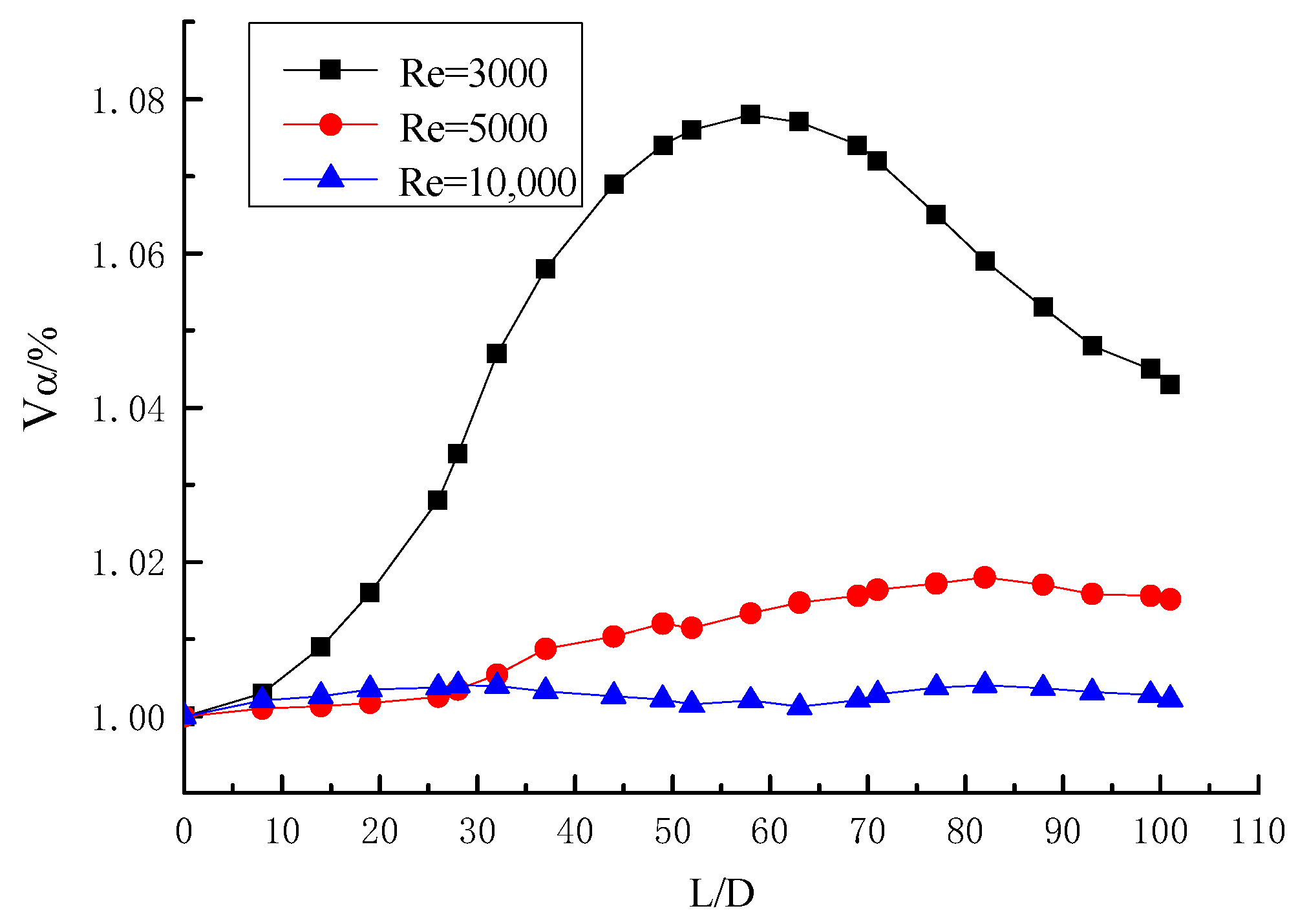
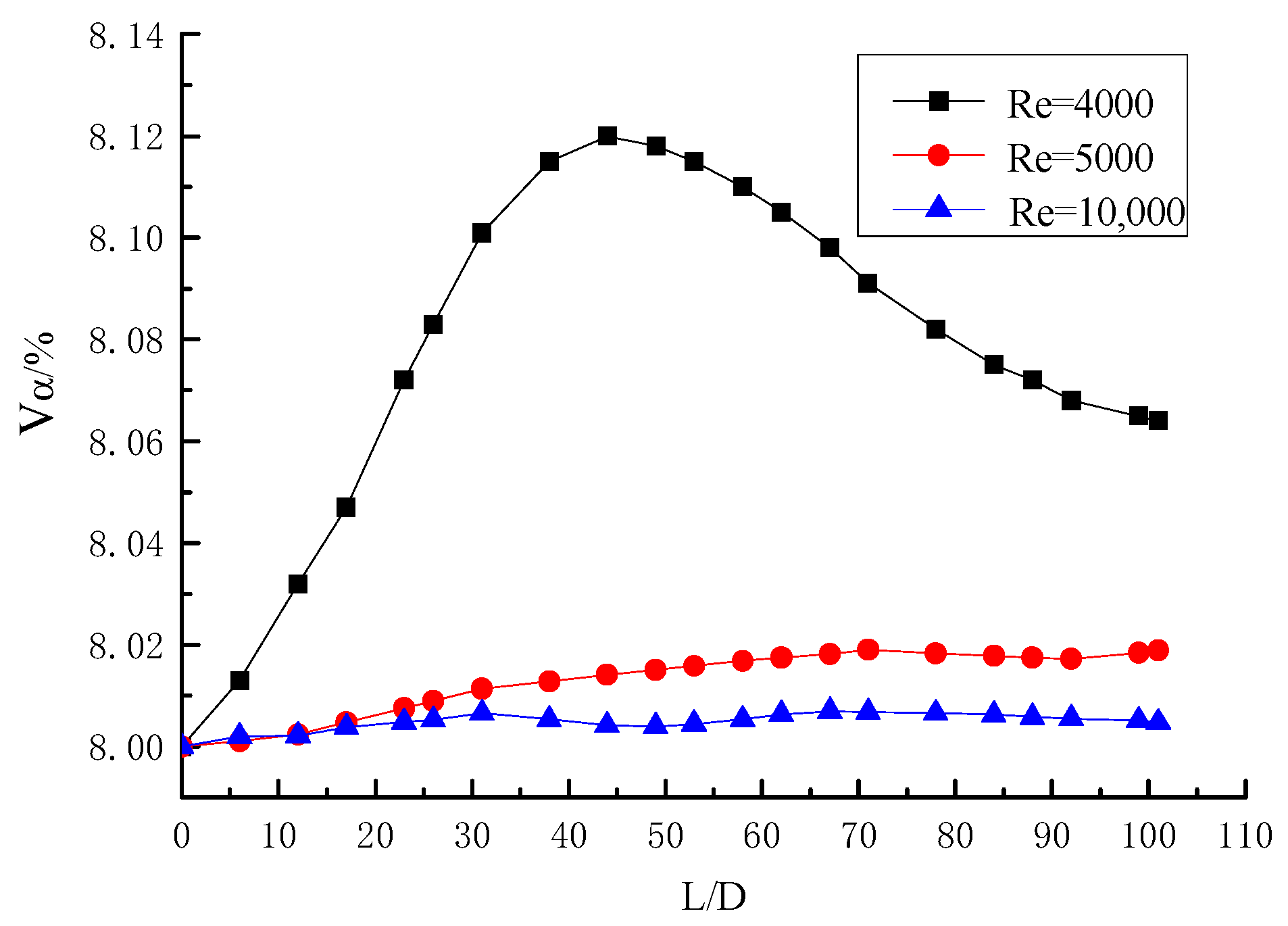
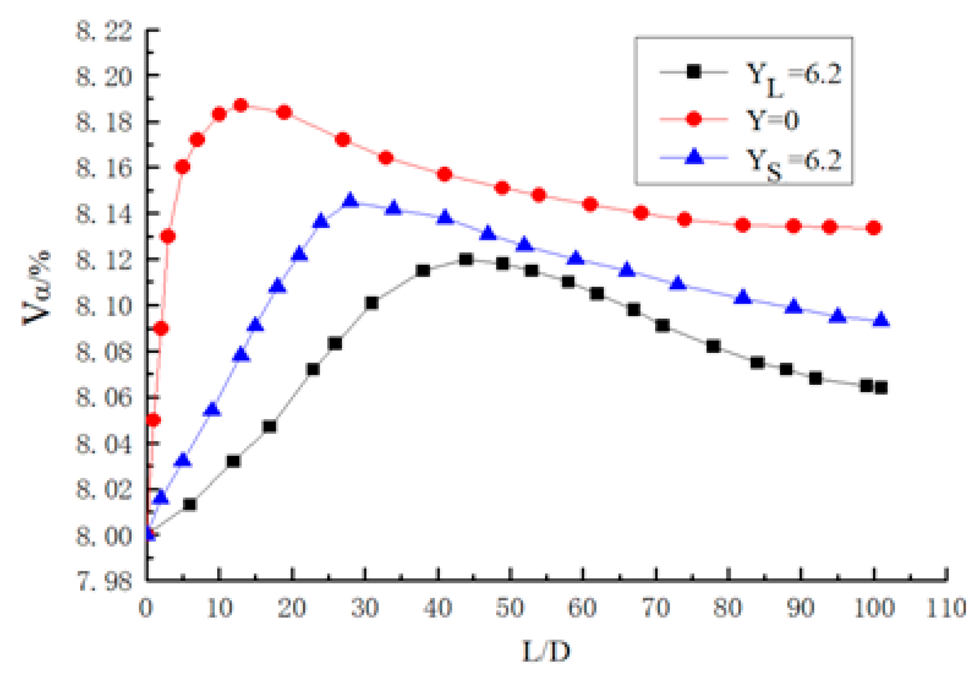
- The Reynolds number is larger, and the particles are less likely to deposit. The particle concentration is larger, and the particle deposition is closer to the pipe. When the twisted rate is 6.2, the initial concentration is between 1% and 8%, and the critical deposition Reynolds number is between 3000 and 5000. The spiral flow carries the hydrate particles a distance that is 3–4 times greater than that without a twisted band.
Author Contributions
Funding
Institutional Review Board Statement
Informed Consent Statement
Data Availability Statement
Conflicts of Interest
References
- Kinnari, K.; Hundseid, J.; Li, X.; Askvik, K.M. Hydrate Management in Practice. J. Chem. Eng. Data 2015, 60, 437–446. [Google Scholar] [CrossRef]
- Chen, B.; Ho, K.; Abakr, Y.A.; Chan, A. Fluid dynamics and heat transfer investigations of swirling decaying flow in an annular pipe Part1: Review, problem description, verification and validation. Int. J. Heat Mass Transf. 2016, 97, 1029–1043. [Google Scholar] [CrossRef]
- Wang, S.; Rao, Y.; Wu, Y.; Wang, X. Experimental Research on Gas-Liquid Two-Phase Spiral Flow in Horizontal Pipe. China Pet. Process. Petrochem. Technol. 2012, 14, 24–32. [Google Scholar]
- Wang, S.L.; Rao, Y.C.; Wei, M.J. Experimental Research on Law of Pressure Drop of Gas-liquid Two-phase Spiral Flow in the Horizontal Pipe. Sci. Technol. Eng. 2013, 13, 659–663. [Google Scholar]
- Zhu, Y.; Wang, S.L.; Shi, X.J. Numerical simulation of pipe spiral flow based on PHOENICS. China Pet. Mach. 2008, 36, 19–22. [Google Scholar]
- Shakutsui, H.; Suzuki, T.; Takagaki, S.; Yamashita, K.; Hayashi, K. Flow patterns in swirling gas-liquid two-phase flow in a vertical pipe. In Proceedings of the 7th International Conference on Multiphase Flow ICMF 2010, Tampa, FL, USA, 30 May–4 June 2010. [Google Scholar]
- Zhang, L.; Zhang, Y. Flow field and flow characteristics along the spiral section of pipe. China Rural Water Hydropower 2011, 9, 48–50. [Google Scholar]
- Rao, Y.; Zheng, Y.; Wang, S. Numerical Simulation of Swirl Flow Rotated by the Vane in the Horizontal Pipe. Fluid Mach. 2016, 44, 17–22. [Google Scholar]
- Kataoka, H.; Shinkai, Y.; Hosokawa, S.; Tomiyama, A. Swirling annular flow in a steam separator. J. Eng. Gas Turbines Power 2009, 131, 032904–032907. [Google Scholar] [CrossRef]
- Kataoka, H.; Shinkai, Y.; Tomiyama, A. Effects of swirler shape on two-phase swirling flow in a steam separator. J. Power Energy Syst. 2009, 3, 347–355. [Google Scholar] [CrossRef][Green Version]
- Kataoka, H.; Shinkai, Y.; Tomiyama, A. Pressure drop in two-phase swirling flow in a steam separator. J. Power Energy Syst. 2009, 3, 382–392. [Google Scholar] [CrossRef]
- Kanizawa, F.T.; Hernandes, R.S.; Moraes, A.U.; Ribatski, G. A new correlation for single and two-phase flow pressure drop in round tubes with twisted-tape inserts. J. Braz. Soc. Mech. Sci. Eng. 2011, 33, 243–250. [Google Scholar]
- Kanizawa, F.T.; Ribatski, G. Two-phase flow patterns and pressure drop in- side horizontal tubes containing twisted-tape inserts. Int. J. Multiph. Flow 2012, 47, 50–65. [Google Scholar] [CrossRef]
- Song, G.; Li, Y.; Wang, W.; Jiang, K.; Shi, Z.; Yao, S. Numerical simulation of pipeline hydrate slurry flow behavior based on population balance theory. Chem. Ind. Eng. Prog. 2018, 37, 561–568. [Google Scholar]
- Song, G.; Li, Y.; Wang, W.; Jiang, K.; Shi, Z.; Yao, S. Numerical simulation of agglomeration process of hydrate particles in pipeline based on population balance theory. Petrochem. Technol. 2018, 47, 573–582. [Google Scholar]
- Song, G.; Li, Y.; Wang, W.; Jiang, K.; Shi, Z.; Yao, S. Numerical simulation of pipeline hydrate particle agglomeration based on population balance theory. J. Nat. Gas Sci. Eng. 2018, 51, 251–261. [Google Scholar] [CrossRef]
- Song, G.; Li, Y.; Wang, W.; Jiang, K.; Shi, Z.; Yao, S. Numerical simulation of hydrate slurry flow behavior in oil-water systems based on hydrate agglomeration modelling. J. Pet. Sci. Eng. 2018, 169, 393–404. [Google Scholar] [CrossRef]
- Rao, Y.; Li, L.; Wang, S.; Zhao, S.; Zhou, S. Numerical Simulation of Spiral Flow and Heat Transfer in Natural Gas Hydrate Pipelines. Oil-Gasfield Surf. Eng. 2018, 37, 6–11. [Google Scholar]
- Rao, Y.; Li, L.; Wang, S.; Zhao, S.; Zhou, S. Numerical Simulation of Spiral Flow and Heat Transfer of Hydrate Pipe Generated by Impeller. China Pet. Mach. 2018, 46, 120–126. [Google Scholar]
- Rao, Y.; Li, L.; Wang, S.; Zhao, S.; Zhou, S. Experimental Research of Solid Particle Transportation Based on Spiral Flow. Oil-Gasfield Surf. Eng. 2018, 37, 1–5. [Google Scholar]
- Cai, Y.; Rao, Y.; Wang, S. Numerical simulation of spiral transport of hydrate particles. Nat. Gas Ind. 2018, 43, 66–73. [Google Scholar]
- Kai, C.; Rao, Y.; Wang, S. Numerical Simulation of Spiral Flow of Gas Hydrate Particles in Gas Transmission Pipeline. China Pet. Mach. 2017, 45, 107–113. [Google Scholar]
- Liu, W.; Hu, J.; Li, X.; Sun, Z.; Sun, F.; Chu, H. Assessment of hydrate blockage risk in long-distance natural gas transmission pipelines. J. Nat. Gas Sci. Eng. 2018, 60, 256–270. [Google Scholar] [CrossRef]
- Brown, E.P.; Turner, D.; Grasso, G.; Koh, C.A. Effect of wax/anti-agglomerant interactions on hydrate depositing systems. Fuel 2020, 264, 116573. [Google Scholar] [CrossRef]
- Nicholas, J.W.; Koh, C.A.; Sloan, E.D.; Nuebling, L.; He, H.; Horn, B. Measuring hydrate/ice deposition in a f low loop from dissolved water in live liquid condensate. Aiche J. 2009, 55, 1882–1888. [Google Scholar] [CrossRef]
- Di Lorenzo, M.; Aman, Z.M.; Sanchez Soto, G.; Johns, M.; Kozielski, K.A.; May, E.F. Hydrate formation in gas-dominant systems using a single-pass flowloop. Energy Fuels 2014, 28, 3043–3052. [Google Scholar] [CrossRef]
- Arjmandi, H.; Amiri, P.; Pour, M.S. Geometric optimization of a double pipe heat exchanger with combined vortex generator and twisted tape: A CFD and response surface methodology (RSM) study. Therm. Sci. Eng. Prog. 2020, 18, 100514. [Google Scholar] [CrossRef]
- Varma, K.K.; Kishore, P.S.; Mendu, S.S.; Gosh, R. Optimization of performance parameters of a double pipe heat exchanger with cut twisted tapes using CFD and RSM. Chem. Eng. Process. Process Intensif. 2021, 163, 108362. [Google Scholar]


| Particle Concentration (%) | Particle Diameter (m) | Twist with Twist Rate Y | Reynolds Number Re |
|---|---|---|---|
| 1 | 0.01 | 0 | 5000 |
| 2 | 0.02 | 6.2 | 10,000 |
| 4 | 0.03 | 7.4 | 15,000 |
| 6 | 0.06 | 8.8 | 20,000 |
| 8 | 0.06 | 8.8 | 20,000 |
Publisher’s Note: MDPI stays neutral with regard to jurisdictional claims in published maps and institutional affiliations. |
© 2021 by the authors. Licensee MDPI, Basel, Switzerland. This article is an open access article distributed under the terms and conditions of the Creative Commons Attribution (CC BY) license (https://creativecommons.org/licenses/by/4.0/).
Share and Cite
Rao, Y.; Li, L.; Wang, S.; Zhao, S.; Zhou, S. Numerical Simulation Study on Flow Laws and Heat Transfer of Gas Hydrate in the Spiral Flow Pipeline with Long Twisted Band. Entropy 2021, 23, 489. https://doi.org/10.3390/e23040489
Rao Y, Li L, Wang S, Zhao S, Zhou S. Numerical Simulation Study on Flow Laws and Heat Transfer of Gas Hydrate in the Spiral Flow Pipeline with Long Twisted Band. Entropy. 2021; 23(4):489. https://doi.org/10.3390/e23040489
Chicago/Turabian StyleRao, Yongchao, Lijun Li, Shuli Wang, Shuhua Zhao, and Shidong Zhou. 2021. "Numerical Simulation Study on Flow Laws and Heat Transfer of Gas Hydrate in the Spiral Flow Pipeline with Long Twisted Band" Entropy 23, no. 4: 489. https://doi.org/10.3390/e23040489
APA StyleRao, Y., Li, L., Wang, S., Zhao, S., & Zhou, S. (2021). Numerical Simulation Study on Flow Laws and Heat Transfer of Gas Hydrate in the Spiral Flow Pipeline with Long Twisted Band. Entropy, 23(4), 489. https://doi.org/10.3390/e23040489