Figure 1.
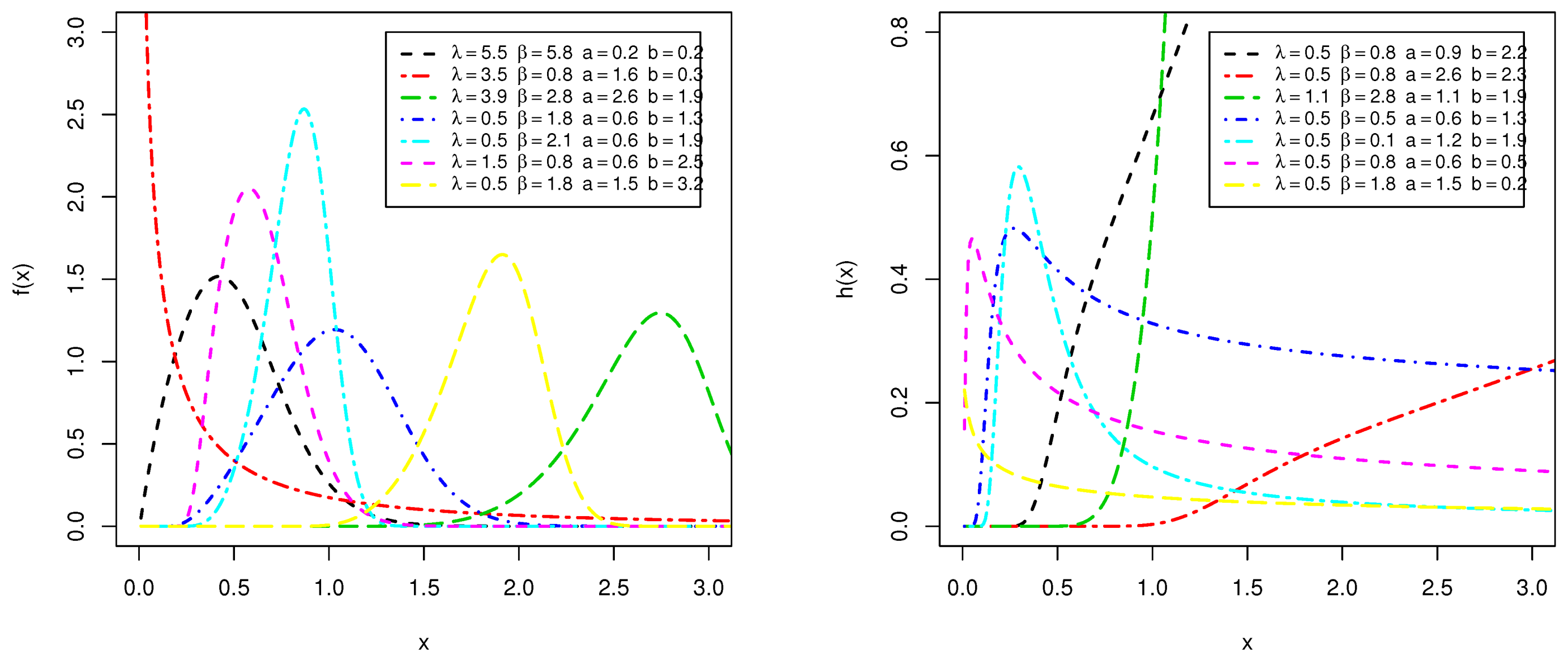
The various plots of PDF (left panel) and HRF (right panel) for Type I HLOWFr distribution.
Figure 1.
The various plots of PDF (left panel) and HRF (right panel) for Type I HLOWFr distribution.
Figure 2.
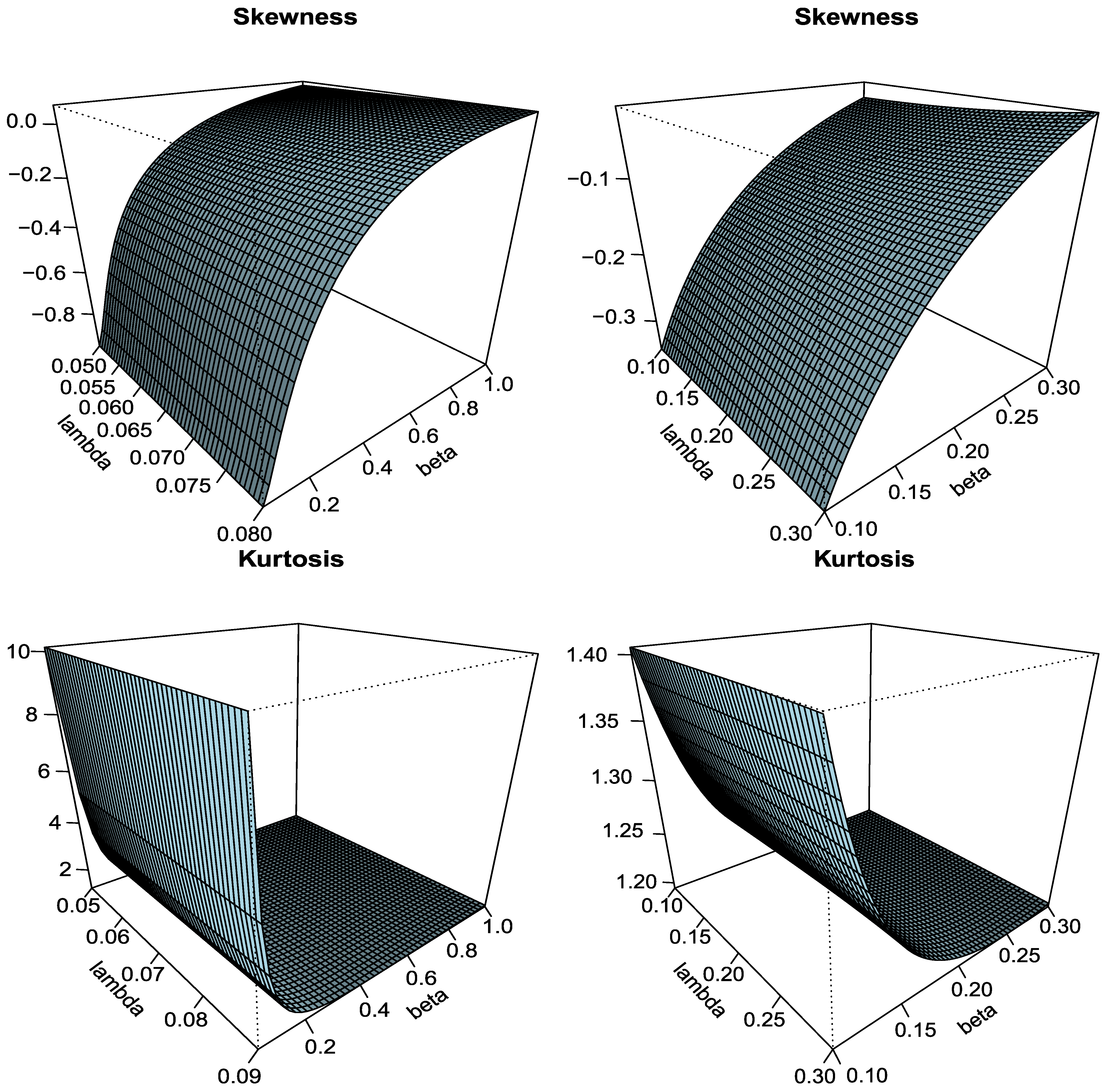
The various plots of skewness and kurtosis for Type I HLOWFr distribution.
Figure 2.
The various plots of skewness and kurtosis for Type I HLOWFr distribution.
Figure 3.
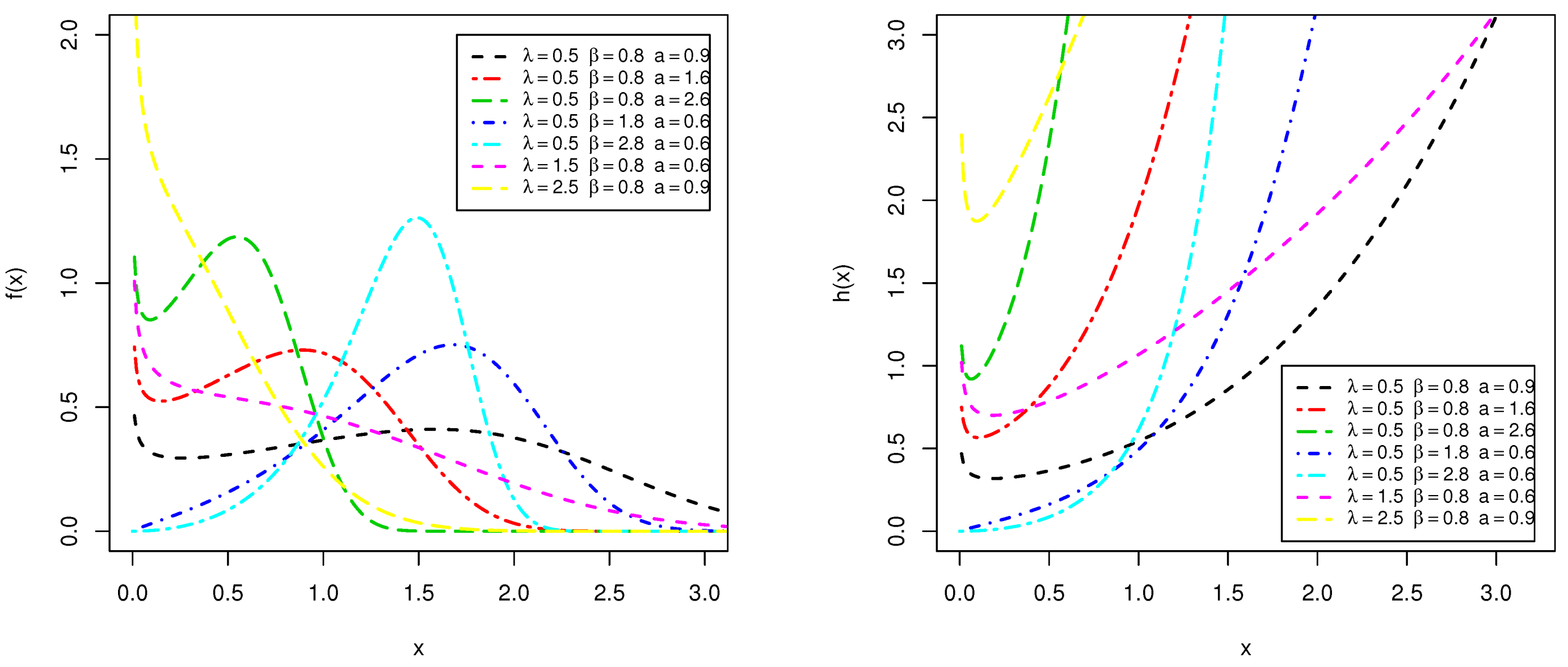
The various plots of PDF (left panel) and HRF (right panel) for Type I HLOWEx distribution.
Figure 3.
The various plots of PDF (left panel) and HRF (right panel) for Type I HLOWEx distribution.
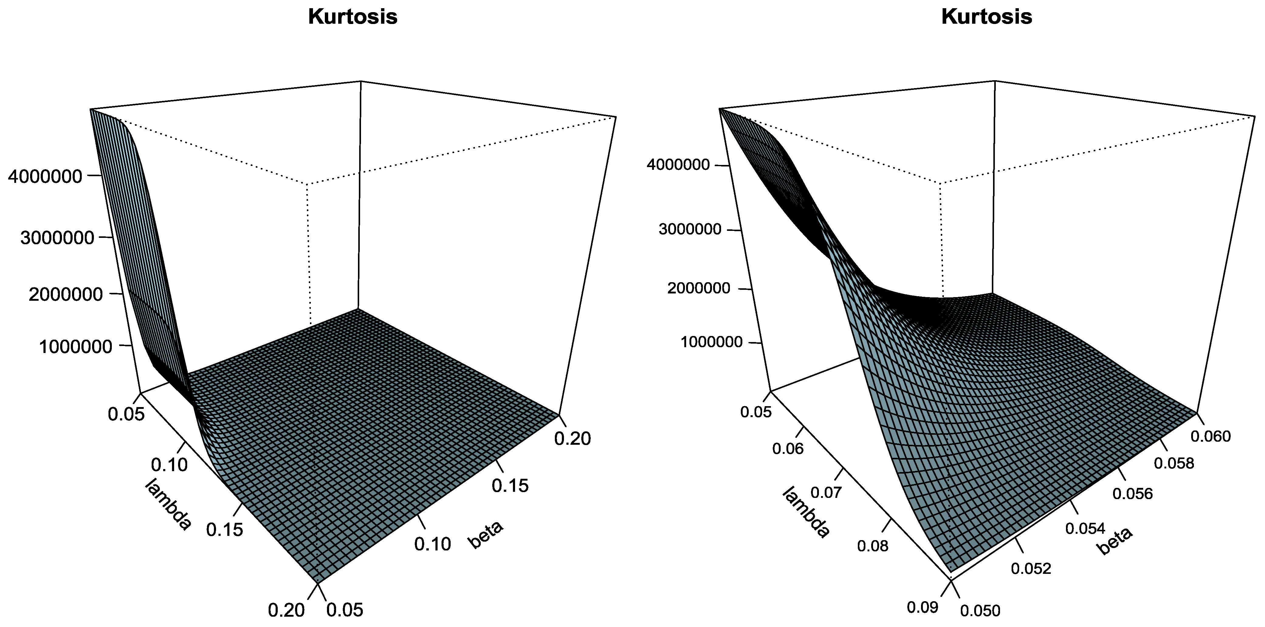
Figure 4.
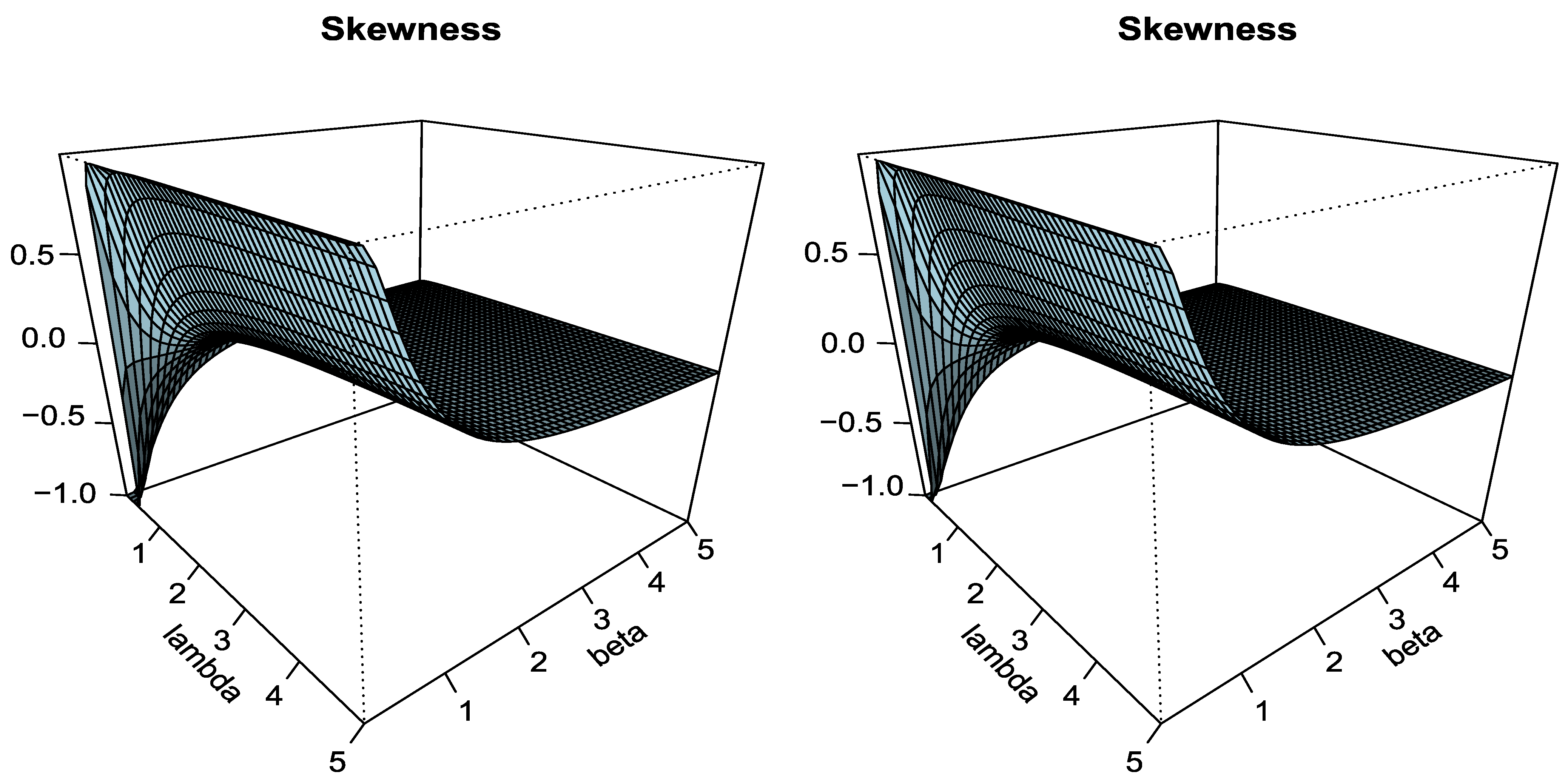
The plots of skewness and kurtosis for Type I HLOWEx distribution.
Figure 4.
The plots of skewness and kurtosis for Type I HLOWEx distribution.
Figure 5.
MCMC diagnostic plots for the parameters of Type I HLOWFr distribution.
Figure 5.
MCMC diagnostic plots for the parameters of Type I HLOWFr distribution.
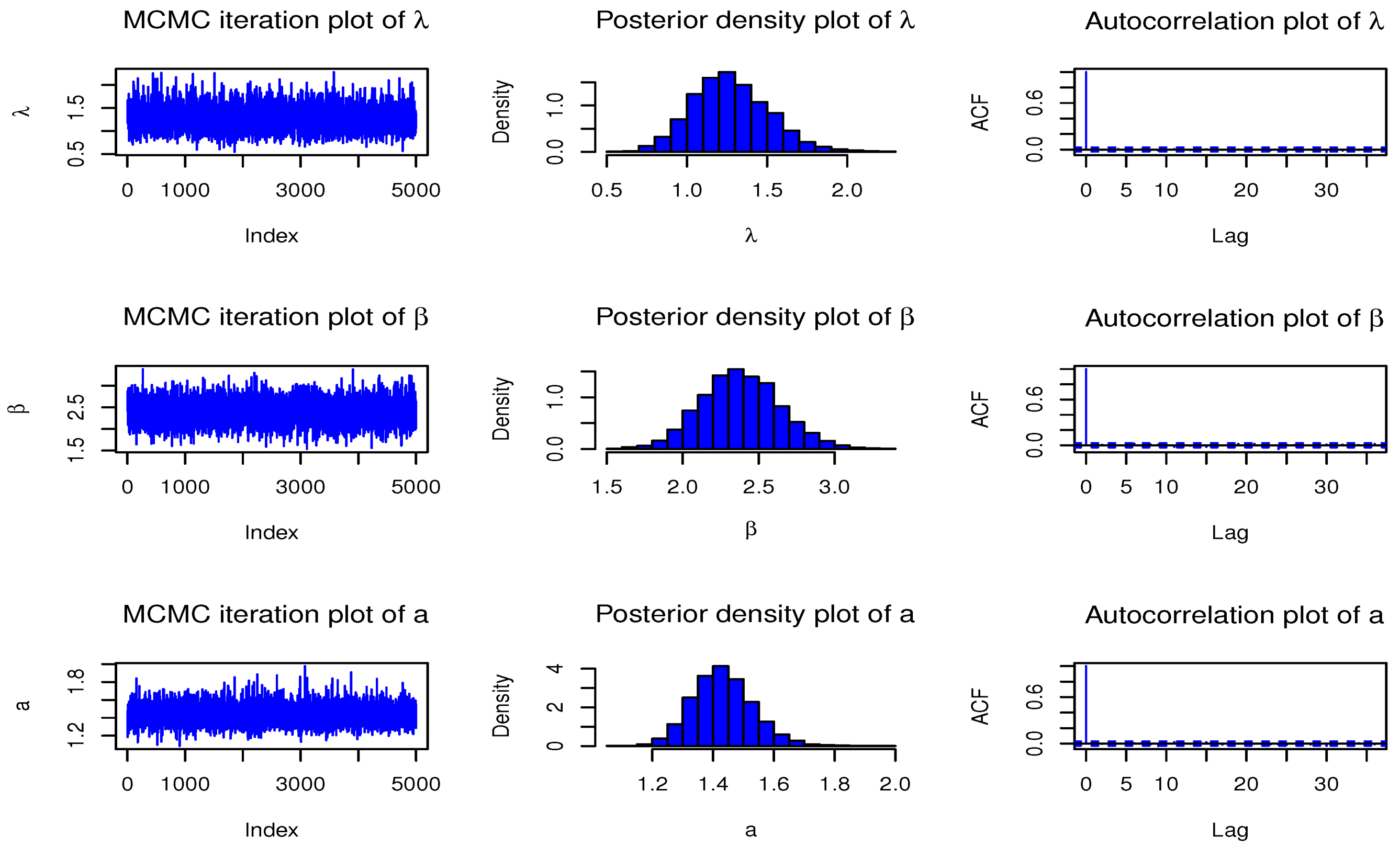
Figure 6.
MCMC diagnostic plots for the parameters of Type I HLOWEx distribution.
Figure 6.
MCMC diagnostic plots for the parameters of Type I HLOWEx distribution.
Figure 7.
The AB and MSE of the Type I HLOWFr based on MLE method.
Figure 7.
The AB and MSE of the Type I HLOWFr based on MLE method.
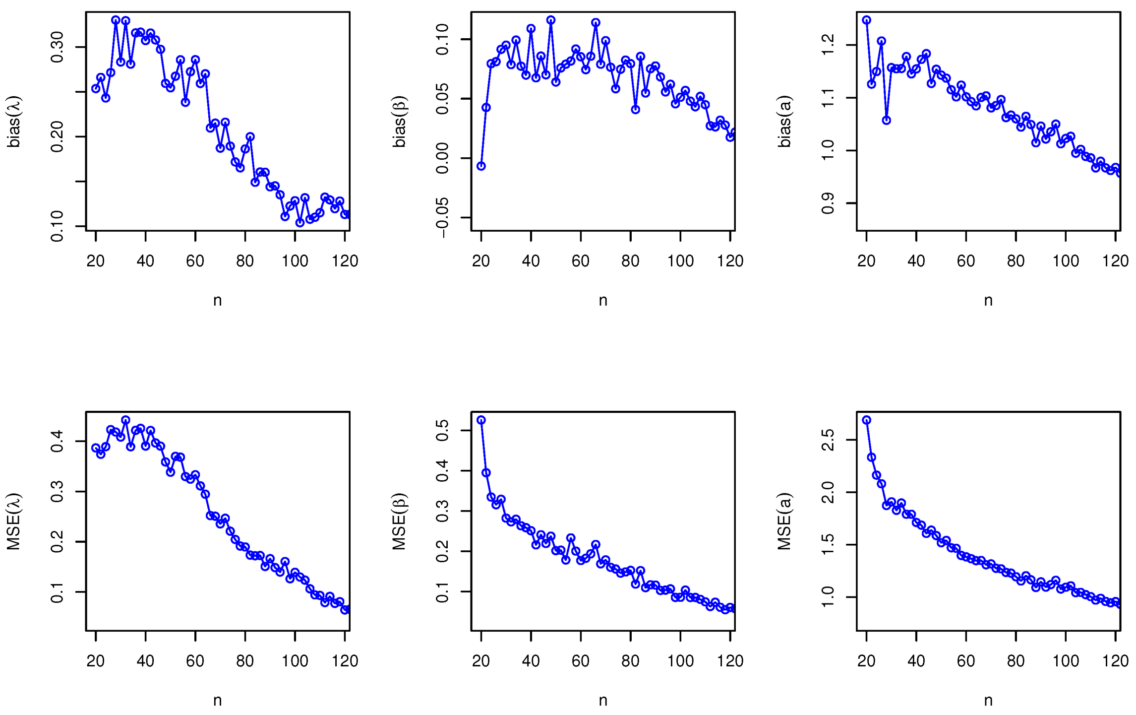
Figure 8.
The AB and MSE of the Type I HLOWEx based on MLE method.
Figure 8.
The AB and MSE of the Type I HLOWEx based on MLE method.
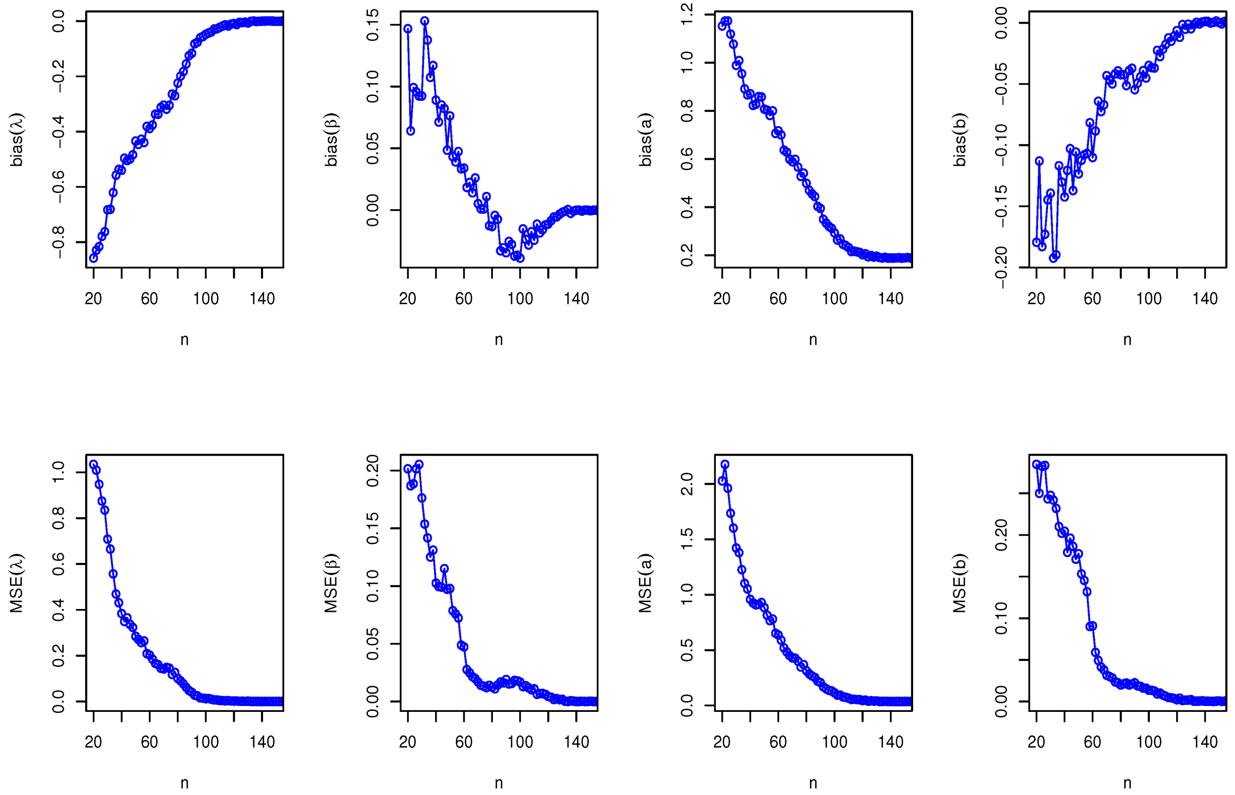
Figure 9.
The AB and MSE of the Type I HLOWFr based on LSE method.
Figure 9.
The AB and MSE of the Type I HLOWFr based on LSE method.
Figure 10.
The AB and MSE of the Type I HLOWEx based on LSE method.
Figure 10.
The AB and MSE of the Type I HLOWEx based on LSE method.
Figure 11.
The AB and MSE of the Type I HLOWFr based on BE with IP method.
Figure 11.
The AB and MSE of the Type I HLOWFr based on BE with IP method.
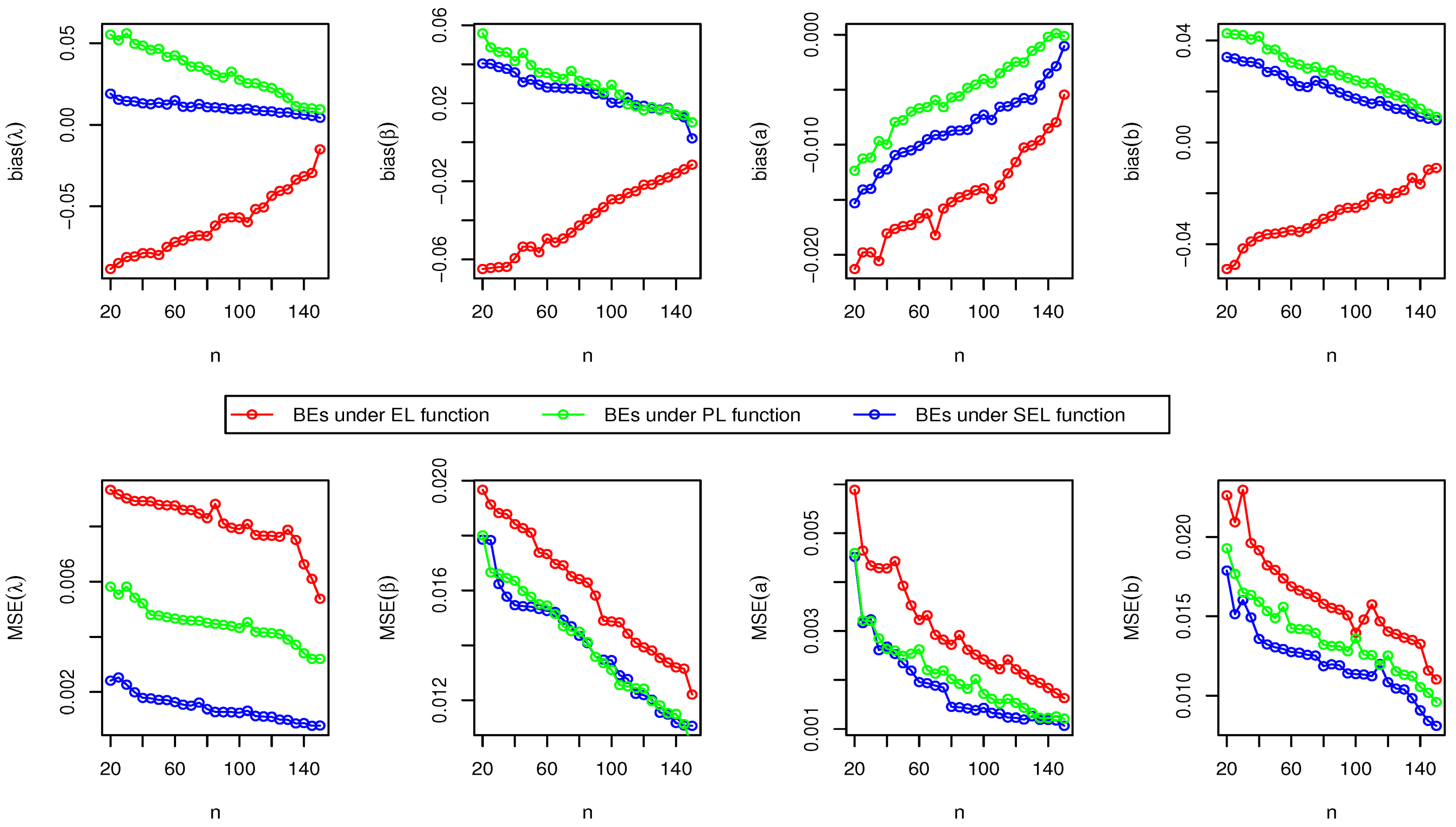
Figure 12.
The AB and MSE of the Type I HLOWEx based on BE with IP method.
Figure 12.
The AB and MSE of the Type I HLOWEx based on BE with IP method.
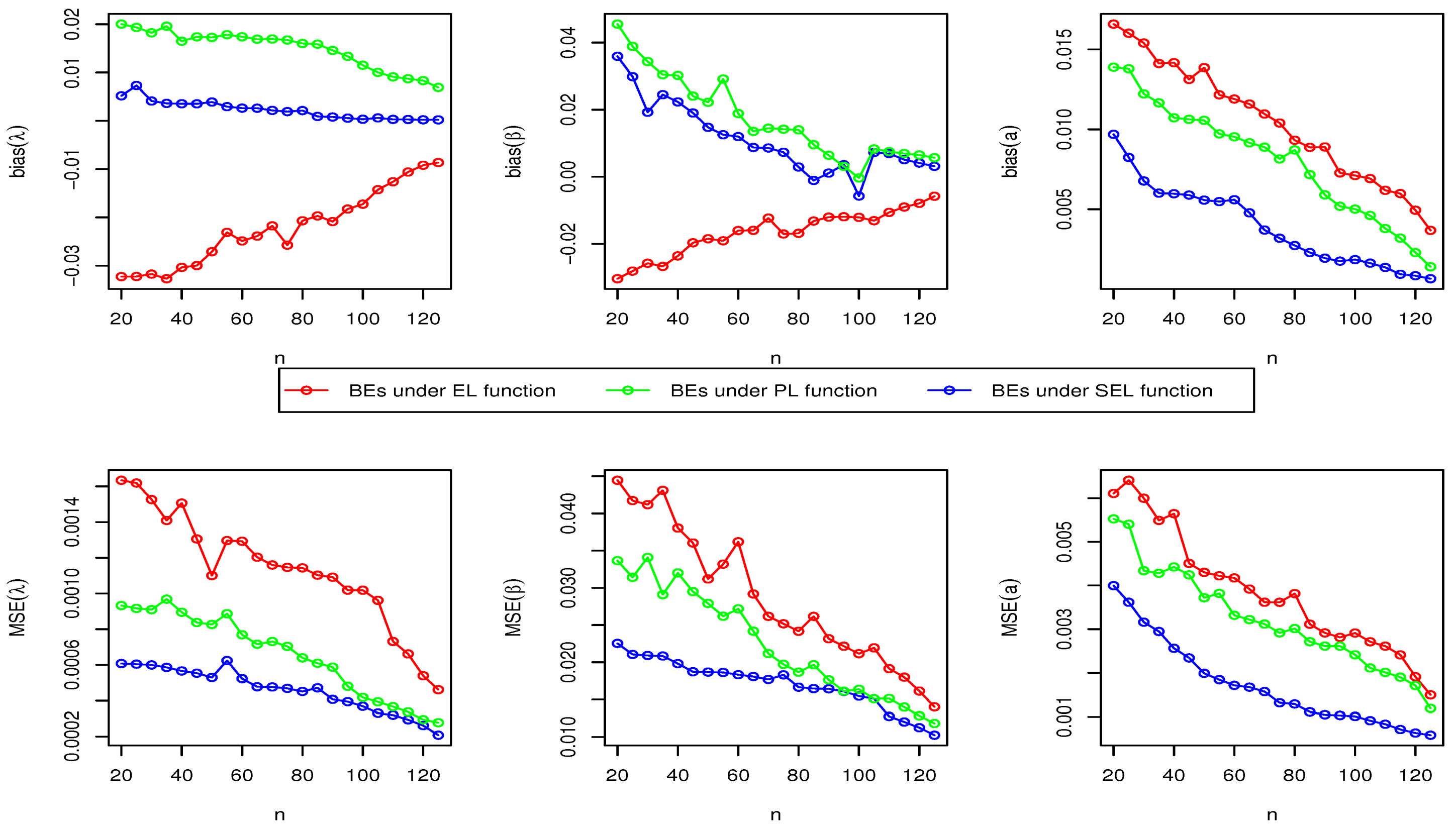
Figure 13.
The AB and MSE of the Type I HLOWFr based on BE with NIP method.
Figure 13.
The AB and MSE of the Type I HLOWFr based on BE with NIP method.
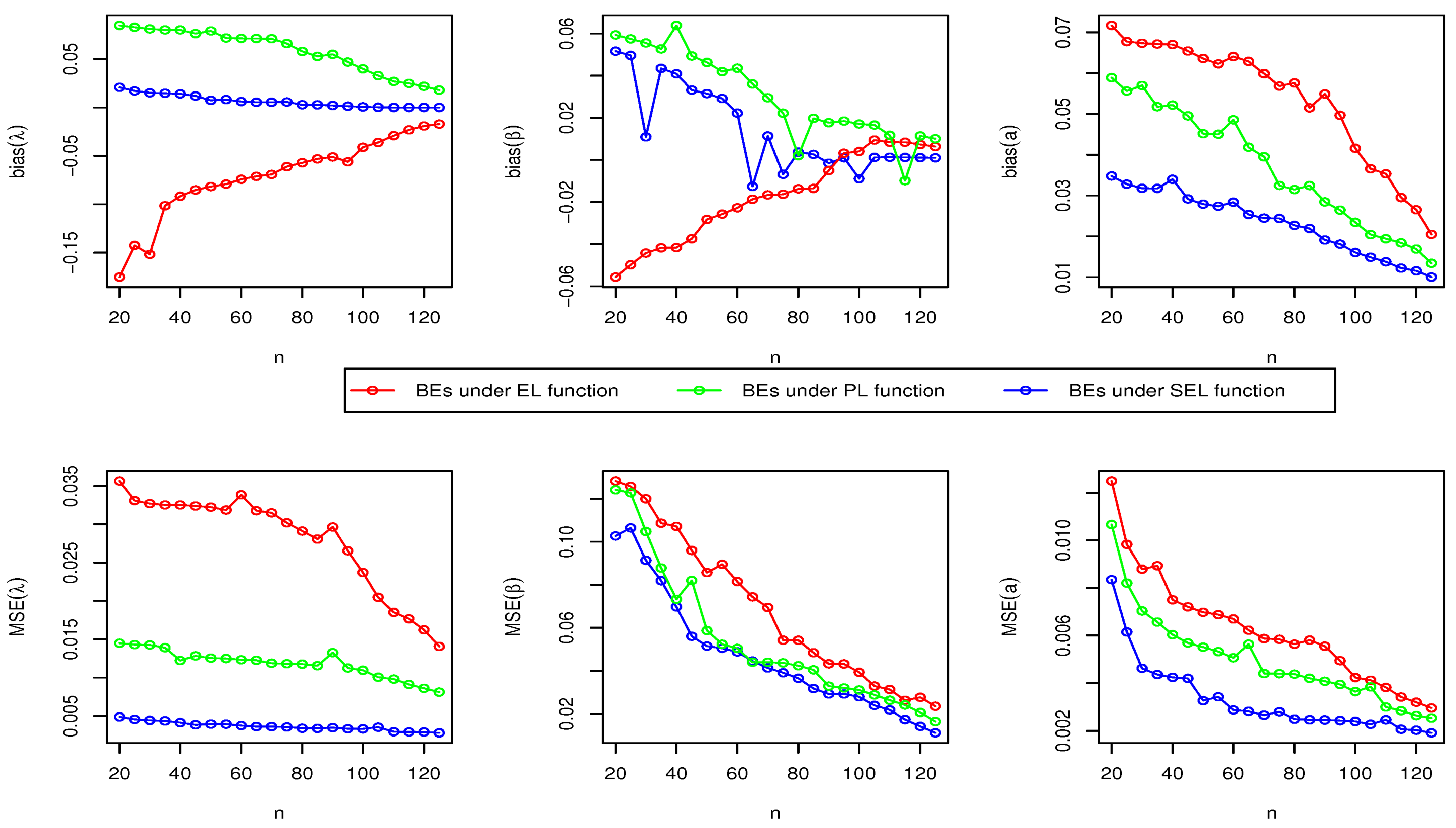
Figure 14.
The AB and MSE of the Type I HLOWEx based on BE with NIP method.
Figure 14.
The AB and MSE of the Type I HLOWEx based on BE with NIP method.
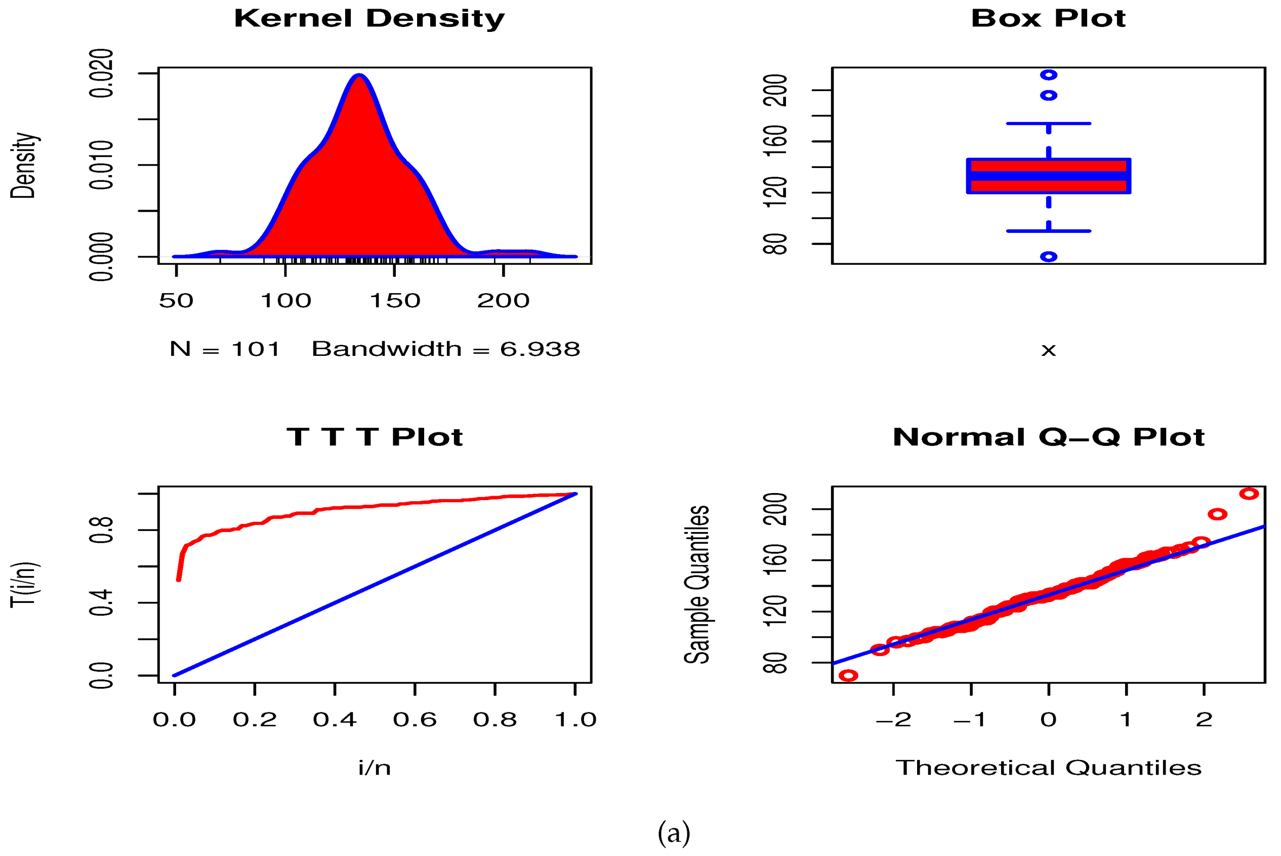
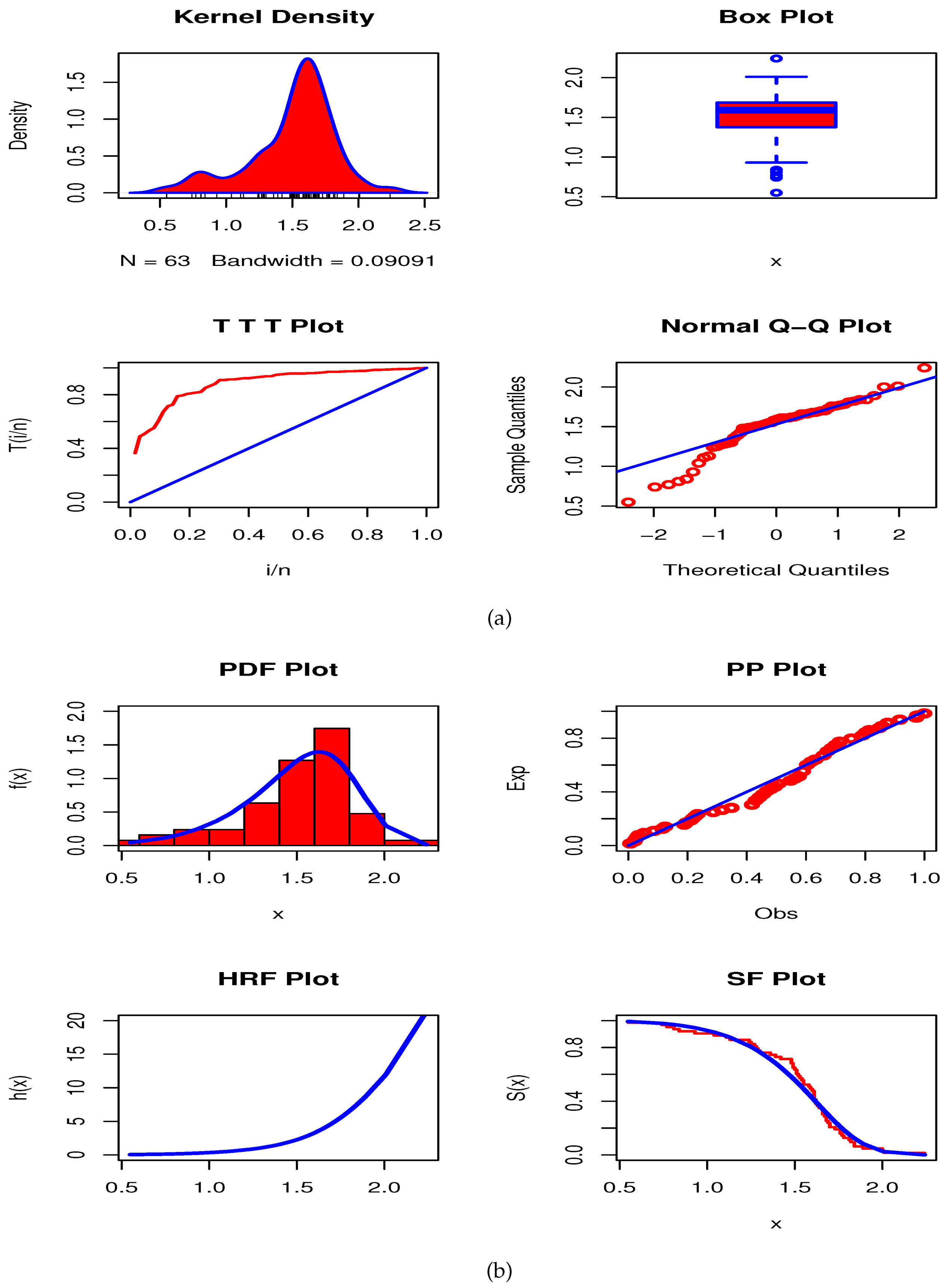
Figure 15.
Plots for AmCs data based on the Type I HLOWFr model.
Figure 15.
Plots for AmCs data based on the Type I HLOWFr model.
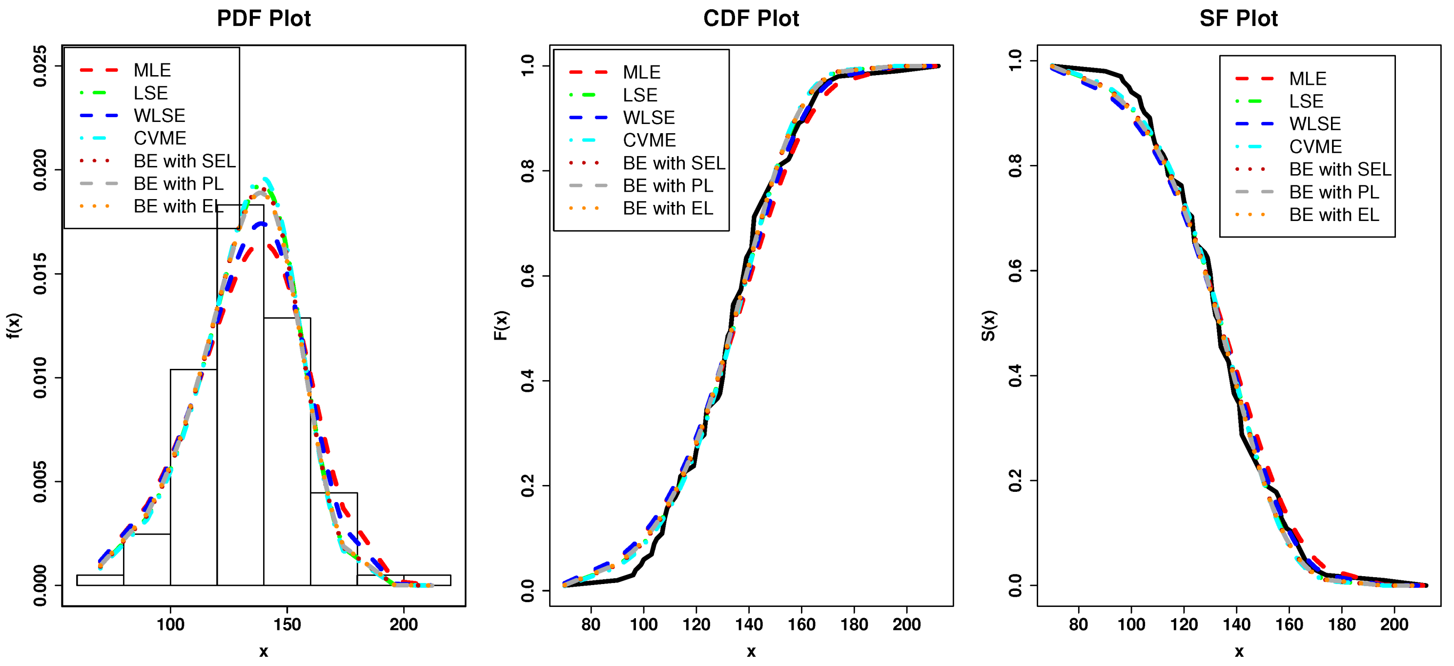
Figure 16.
The fitted plots of the Type I HLOWFr parameters under the various method of estimation based on AmCs data.
Figure 16.
The fitted plots of the Type I HLOWFr parameters under the various method of estimation based on AmCs data.
Figure 17.
Plots for GsFr data based on the Type I HLOWEx model.
Figure 17.
Plots for GsFr data based on the Type I HLOWEx model.
Figure 18.
The fitted plots of the Type I HLOWEx parameters under the various method of estimation based on GsFr data.
Figure 18.
The fitted plots of the Type I HLOWEx parameters under the various method of estimation based on GsFr data.
Table 1.
Some special models of Type I HLOW-G family.
Table 1.
Some special models of Type I HLOW-G family.
| | Reduced Distribution | |
|---|
| | Type I HLOW-exponential | a |
| | Type I HLOW-Rayleigh | a |
| | Type I HLOW-Lindely | a |
| | Type I HLOW-Weibull | |
| | Type I HLOW-Fréchet | |
| | Type I HLOW-Lomax | |
Table 2.
The MLEs with their (SEs) and KS with its p-value for AmCs data.
Table 2.
The MLEs with their (SEs) and KS with its p-value for AmCs data.
| Model | | | | | KS | p-Value |
|---|
| Type I HLOWFr | | | | | | |
| | | | | | − | − |
| ToLFr | | | | | | |
| | | | | | − | − |
| TrFr | | − | | | | |
| | | − | | | − | − |
| ETrFr | | | | | | |
| | | | | | − | − |
| GuFr | | | | | | |
| | | | | | − | − |
| TIGFr | | | | | | |
| | | | | | − | − |
| EFr | − | | | | | |
| | − | | | | − | − |
| Fr | − | − | | | | |
| | − | − | | | − | − |
Table 3.
The GOF Statistics for the AmCs data.
Table 3.
The GOF Statistics for the AmCs data.
| Model | −logL | AkIC | CAkIC | BsIC | HQIC | AD | CvM | DF |
|---|
| Type I HLOWFr | | | | | | | | 4 |
| ToLFr | | | | | | | | 4 |
| TrFr | | | | | | | | 3 |
| ETrFr | | | | | | | | 4 |
| GuFr | | | | | | | | 4 |
| TIGFr | | | | | | | | 4 |
| EFr | | | | | | | | 3 |
| Fr | | | | | | | | 2 |
Table 4.
Different estimation techniques for the Type I HLOWFr parameters with KS, (SE) and p-values for the AmCs data.
Table 4.
Different estimation techniques for the Type I HLOWFr parameters with KS, (SE) and p-values for the AmCs data.
| Method ↓Estimator→ | | | | | KS | p-Value |
|---|
| LSE | | | | | | |
| WLSE | | | | | | |
| CVME | | | | | | |
| BE with SEL function | | | | | | |
| BE with PL function | | | | | | |
| BE with EL function | | | | | | |
Table 5.
The MLEs with their (SEs) and KS with its p-value for the GsFr data.
Table 5.
The MLEs with their (SEs) and KS with its p-value for the GsFr data.
| Model | | | | | KS | p-Value |
|---|
| Type I HLOWEx | | | | − | | |
| | (2.4146) | (1.6865) | (0.7175) | − | − | − |
| GWEx | | | | 1.9018 | | |
| | (0.0656) | (0.6310) | (3.2469) | (1.2361) | − | − |
| ExOWEx | | | | − | | |
| | (0.6423) | (0.1572) | (0.0121) | − | − | − |
| MoOWEx | | | | − | | |
| | (0.1499) | (1.5824) | (0.6762) | − | − | − |
| OFWEx | | | | − | | |
| | (8.5346) | (2.5169) | (0.5322) | − | − | − |
| ToLEx | | | | − | | |
| | (48.9007) | (0.3207) | (0.2828) | − | − | − |
| OWEx | | | | − | | |
| | (0.0185) | (0.7872) | (0.3879) | − | − | − |
| OBuXEx | | − | | − | | |
| | (0.5366) | − | (0.02004) | − | − | − |
| KuEx | | | | − | | |
| | (0.7092) | | | − | − | − |
| OLogLEx | | − | | − | | |
| | (0.6555) | − | (0.0118) | − | − | − |
| OChEx | | | | − | | |
| | (189.9452) | (0.9314) | (0.1366) | − | − | − |
| GuEx | | | | − | | |
| | (9.9112) | (0.4542) | (0.6979) | − | − | − |
| EEx | − | | | − | | |
| | − | (9.5154) | (0.2379) | − | − | − |
| Ex | − | − | | − | | |
| | − | − | (0.0836) | − | − | − |
Table 6.
The GOF Statistics for the GsFr data.
Table 6.
The GOF Statistics for the GsFr data.
| Model | | AkIC | CAkIC | BsIC | HQIC | AD | CvM | DF |
|---|
| Type I HLOWEx | | | | | | | | 3 |
| GWEx | | | | | | | | 4 |
| ExOWEx | | | | | | | | 3 |
| MoOWEx | | | | | | | | 3 |
| OFWEx | | | | | | | | 3 |
| ToLEx | | | | | | | | 3 |
| OWEx | | | | | | | | 3 |
| OBuXEx | | | | | | | | 2 |
| KuEx | | | | | | | | 3 |
| OLogLEx | | | | | | | | 2 |
| OChEx | | | | | | | | 3 |
| GuEx | | | | | | | | 3 |
| EEx | | | | | | | | 2 |
| Ex | | | | | | | | 1 |
Table 7.
Different estimation techniques for the Type I HLOWEx parameters with KS, (SE) and p-values for the GsFr data.
Table 7.
Different estimation techniques for the Type I HLOWEx parameters with KS, (SE) and p-values for the GsFr data.
| Method ↓ Estimator → | | | | KS | p-Value |
|---|
| LSE | | | | | |
| WLSE | | | | | |
| CVME | | | | | |
| BE with SEL function | | | | | |
| BE with PL function | | | | | |
| BE with EL function | | | | | |
Table 8.
Empirical and theoretical descriptive statistics for data sets I and II.
Table 8.
Empirical and theoretical descriptive statistics for data sets I and II.
| Data Set | Measure | Mean | Variance | Skewness | Kurtosis | Index of Dispersion |
|---|
| I | Empirical | | | | | (over-dispersed) |
| | Theoretical | | | | | (over-dispersed) |
| II | Empirical | | | | | (under-dispersed) |
| | Theoretical | | | | | (under-dispersed) |
