A New Family of Continuous Probability Distributions

 ,
,  ,
,  ,
,  and
and 
Abstract
1. Introduction and Genesis
2. Copula
2.1. BvPGE-G Type via CCp
2.2. BvPGE-G Type via RECp
2.3. BvPGE-G Type via FGMCp
2.4. BvPGE-G Type via Modified FGMCp
2.5. BvPGE-G Type via Ali-Mikhail-Haq Copula
3. Properties
3.1. Expanding the Univariate PDF
3.2. Convex-Concave Analysis
3.3. Moments
3.4. Moment-Generating Function (MGF)
3.5. Incomplete Moments (IM)
3.6. Residual Life (RL) and Reversed Residual Life (RRL)
3.7. Mathematical Results and Numerical Analysis for Two Special Models
4. Numerical Analysis for Some Measures
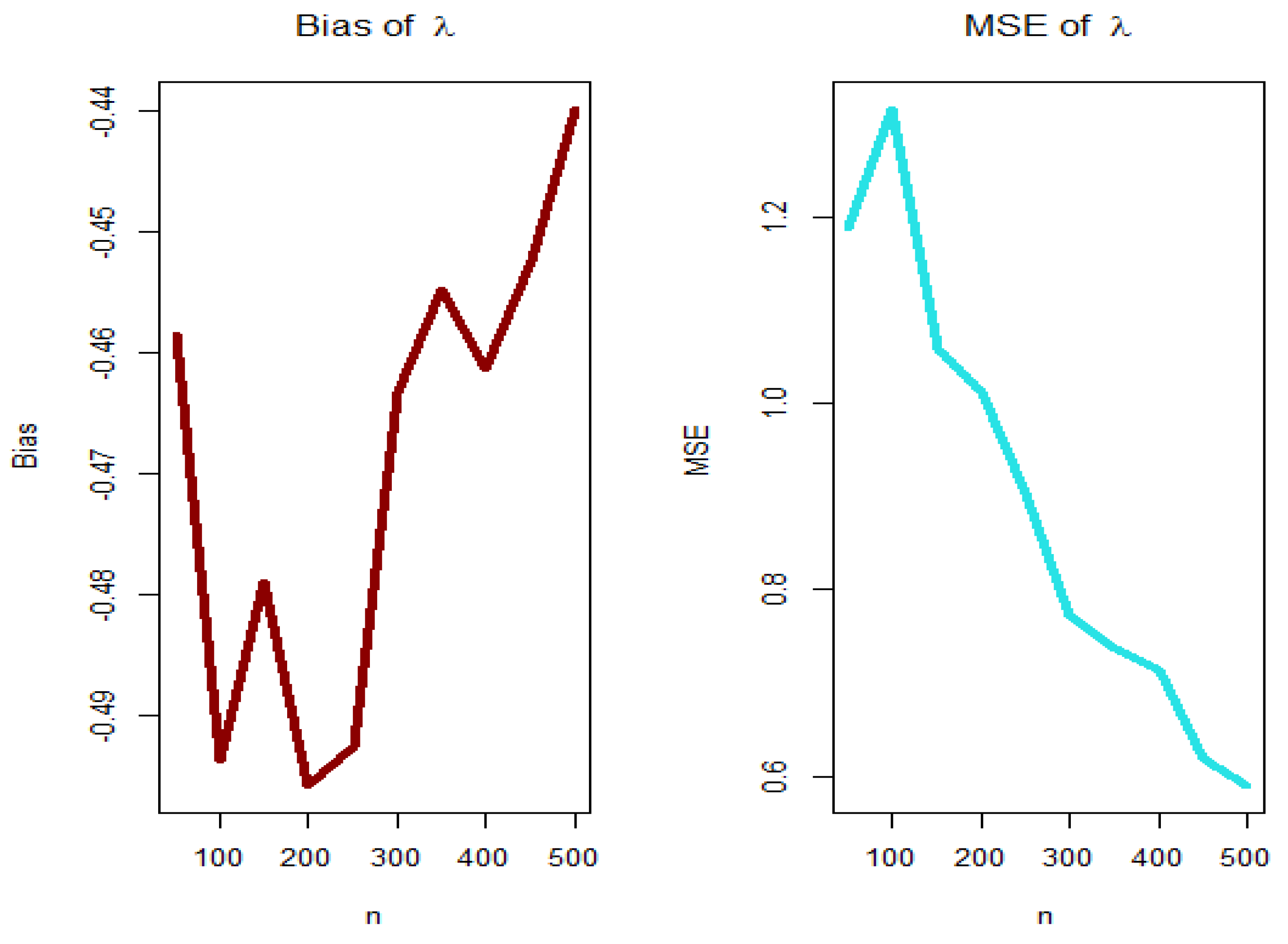
5. Estimation Method and Assessment
5.1. The Maximum Likelihood Estimation (MLE) Method
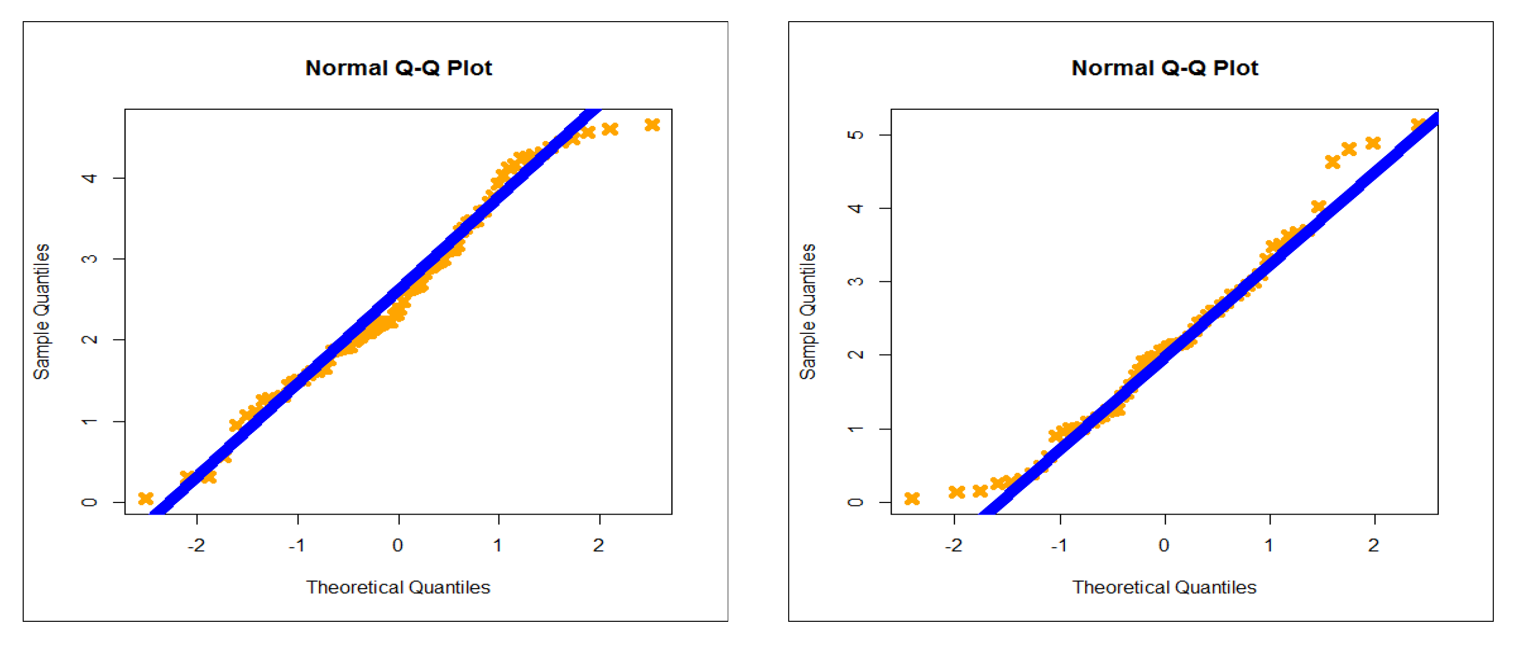
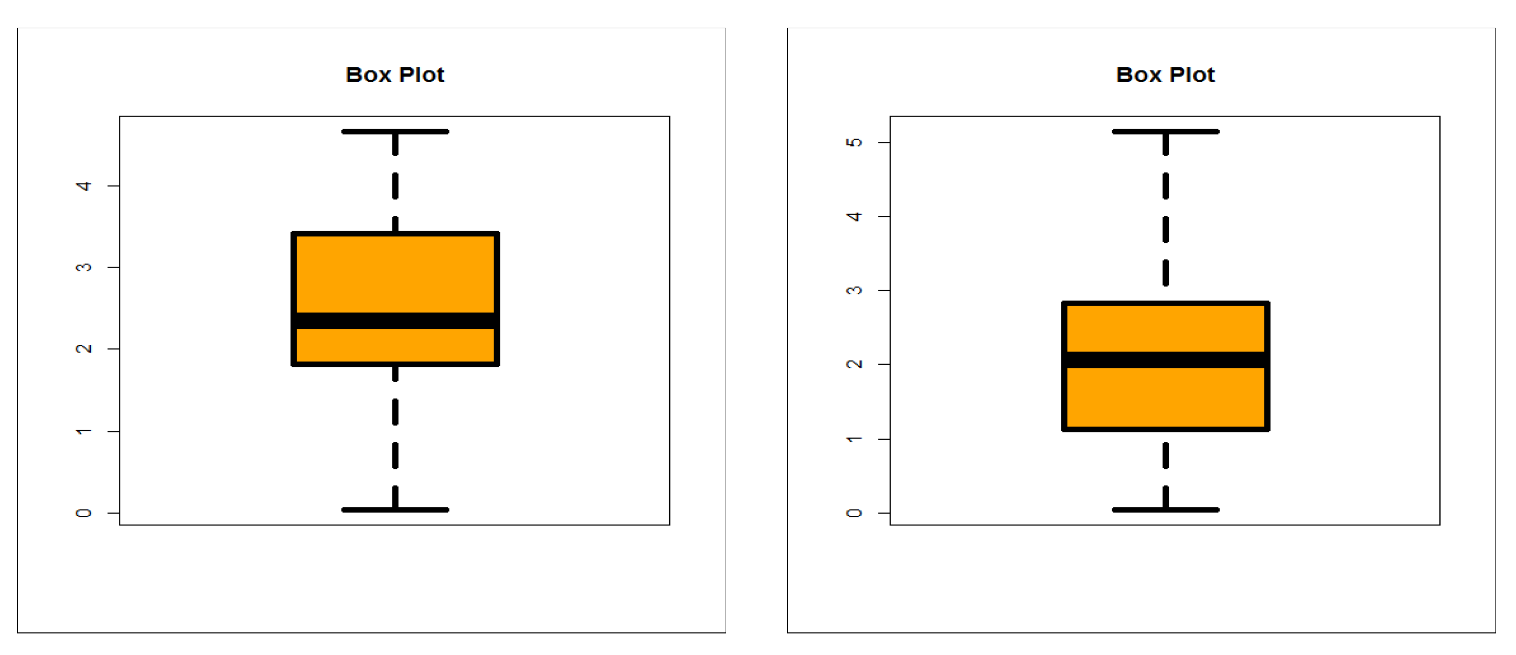
5.2. Graphical Assessment
6. Modeling Failure and Service Times

| N. | Model | Abbreviation | Author |
|---|---|---|---|
| 1 | Special generalized mixture-PII | SGMPII | [29] |
| 2 | Odd log-logistic-PII | OLLPII | [30] |
| 3 | Reduced OLL-PII | ROLLPII | [30] |
| 4 | Reduced Burr–Hatke-PII | RBHPII | [31] |
| 5 | Transmuted Topp–Leone-PII | TTLPII | [32] |
| 6 | Reduced TTL-PII | RTTLPII | [32] |
| 7 | Gamma-PII | GamPII | [33] |
| 8 | Kumaraswamy-PII | KumPII | [34] |
| 9 | McDonald-PII | McPII | [34] |
| 10 | Beta-PII | BPII | [34] |
| 11 | Exponentiated-PII | EPII | [35] |
| 12 | PII | PII | [36] |
| 13 | Proportional reversed hazard rate PII | PRHRPII | New |
7. Conclusions
Author Contributions
Funding
Institutional Review Board Statement
Informed Consent Statement
Data Availability Statement
Acknowledgments
Conflicts of Interest
References
- Maurya, S.K.; Nadarajah, S. Poisson Generated Family of Distributions: A Review. Sankhya 2020, 1–57. [Google Scholar] [CrossRef]
- Bourguignon, M.; Silva, R.B.; Cordeiro, G.M. The Weibull-G family of probability distributions. J. Data Sci. 2014, 12, 53–68. [Google Scholar]
- Ramos, M.W.A.; Marinho, P.R.D.; Cordeiro, G.M.; da Silva, R.V.; Hamedani, G.G. The Kumaraswamy-G Poisson family of distributions. J. Stat. Theory Appl. 2015, 14, 222–239. [Google Scholar]
- Aryal, G.R.; Yousof, H.M. The exponentiated generalized-G Poisson family of distributions. Econ. Qual. Control 2017, 32, 1–17. [Google Scholar] [CrossRef]
- Abouelmagd, T.H.M.; Hamed, M.S.; Handique, L.; Goual, H.; Ali, M.M.; Yousof, H.M.; Korkmaz, M.C. A new class of distributions based on the zero truncated Poisson distribution with properties and applications. J. Nonlinear Sci. Appl. 2019, 12, 152–164. [Google Scholar] [CrossRef]
- Alizadeh, M.; Yousof, H.M.; Rasekhi, M.; Altun, E. The odd log-logistic Poisson-G Family of distributions. J. Math. Ext. 2019, 12, 81–104. [Google Scholar]
- Korkmaz, M.C.; Yousof, H.M.; Hamedani, G.G.; Ali, M.M. The Marshall–Olkin generalized G Poisson family of distributions. Pak. J. Stat. 2018, 34, 251–267. [Google Scholar]
- Yousof, H.M.; Afify, A.Z.; Alizadeh, M.; Hamedani, G.G.; Jahanshahi, S.M.A.; Ghosh, I. The generalized transmuted Poisson-G family of Distributions. Pak. J. Stat. Oper. Res. 2018, 14, 759–779. [Google Scholar] [CrossRef]
- Yousof, H.M.; Mansoor, M.; Alizadeh, M.; Afify, A.Z.; Ghosh, I. The Weibull-G Poisson family for analyzing lifetime data. Pak. J. Stat. Oper. Res. 2020, 16, 131–148. [Google Scholar] [CrossRef]
- Farlie, D.J.G. The performance of some correlation coefficients for a general bivariate distribution. Biometrika 1960, 47, 307–323. [Google Scholar] [CrossRef]
- Morgenstern, D. Einfache beispiele zweidimensionaler verteilungen. Mitteilingsbl. Math. Stat. 1956, 8, 234–235. [Google Scholar]
- Gumbel, E.J. Bivariate exponential distributions. J. Am. Stat. Assoc. 1960, 55, 698–707. [Google Scholar] [CrossRef]
- Gumbel, E.J. Bivariate logistic distributions. J. Am. Stat. Assoc. 1961, 56, 335–349. [Google Scholar] [CrossRef]
- Johnson, N.L.; Kotz, S. On some generalized Farlie-Gumbel-Morgenstern distributions. Commun. Stat. Theory 1975, 4, 415–427. [Google Scholar] [CrossRef]
- Johnson, N.L.; Kotz, S. On some generalized Farlie-Gumbel-Morgenstern distributions-II: Regression, correlation and further generalizations. Commun. Stat. Theory 1977, 6, 485–496. [Google Scholar] [CrossRef]
- Balakrishnan, N.; Lai, C.D. Continuous Bivariate Distributions; Springer Science & Business Media: Berlin/Heidelberg, Germany, 2009. [Google Scholar]
- Nelsen, R.B. An Introduction to Copulas; Springer Science & Business Media: Berlin/Heidelberg, Germany, 2007. [Google Scholar]
- Pougaza, D.B.; Djafari, M.A. Maximum entropies copulas. In Proceedings of the 30th international workshop on Bayesian inference and maximum Entropy methods in Science and Engineering, Chamonix, France, 4–9 July 2010; pp. 329–336. [Google Scholar]
- Ali, M.M.; Mikhail, N.N.; Haq, M.S. A class of bivariate distributions including the bivariate logistic. J. Multivar. Anal. 1978, 8, 405–412. [Google Scholar] [CrossRef]
- Murthy, D.N.P.; Xie, M.; Jiang, R. Weibull Models; John Wiley & Sons: Hoboken, NJ, USA, 2004. [Google Scholar]
- Yousof, H.M.; Afify, A.Z.; Abd El Hadi, N.E.; Hamedani, G.G.; Butt, N.S. On six-parameter Fréchet distribution: Properties and applications. Pak. J. Stat. Oper. Res. 2016, 281–299. [Google Scholar] [CrossRef]
- Yousof, H.M.; Afify, A.Z.; Nadarajah, S.; Hamedani, G.; Aryal, G.R. The Marshall-Olkin generalized-G family of distributions with Applications. Statistica 2018, 78, 273–295. [Google Scholar]
- Aryal, G.R.; Ortega, E.M.; Hamedani, G.G.; Yousof, H.M. The Topp-Leone generated Weibull distribution: Regression model, characterizations and applications. Int. J. Stat. Probab. 2017, 6, 126–141. [Google Scholar] [CrossRef]
- Ibrahim, M. The compound Poisson Rayleigh Burr XII distribution: Properties and applications. J. Appl. Probab. Stat. 2020, 15, 73–97. [Google Scholar]
- Altun, E.; Yousof, H.M.; Hamedani, G.G. A new log-location regression model with influence diagnostics and residual analysis. Facta Univ. Ser. 2018, 33, 417–449. [Google Scholar]
- Altun, E.; Yousof, H.M.; Chakraborty, S.; Handique, L. Zografos-Balakrishnan. Burr XII distribution: Regression modeling and applications. Int. J. Math. Stat. 2018, 19, 46–70. [Google Scholar]
- Elgohari, H.; Yousof, H.M. New Extension of Weibull Distribution: Copula, Mathematical Properties and Data Modeling. Stat. Optim. Inf. Comput. 2020, 8, 972–993. [Google Scholar] [CrossRef]
- Ibrahim, M.; Altun, E.; Yousof, H.M. A new distribution for modeling lifetime data with different methods of estimation and censored regression modeling. Stat. Optim. Inf. Comput. 2020, 8, 610–630. [Google Scholar] [CrossRef]
- Chesneau, C.; Yousof, H.M. On a special generalized mixture class of probabilistic models. J. Nonlinear Model. Anal. 2021, forthcoming. [Google Scholar]
- Elgohari, H.; Yousof, H.M. A Generalization of Lomax Distribution with Properties, Copula and Real Data Applications. Pak. J. Stat. Oper. Res. 2020, 16, 697–711. [Google Scholar] [CrossRef]
- Yousof, H.M.; Altun, E.; Ramires, T.G.; Alizadeh, M.; Rasekhi, M. A new family of distributions with properties, regression models and applications. J. Stat. Manag. Syst. 2018, 21, 163–188. [Google Scholar] [CrossRef]
- Yousof, H.M.; Alizadeh, M.; Jahanshahi, S.M.A.; Ramires, T.G.; Ghosh, I.; Hamedani, G.G. The transmuted Topp-Leone G family of distributions: Theory, characterizations and applications. J. Data Sci. 2017, 15, 723–740. [Google Scholar]
- Cordeiro, G.M.; Ortega, E.M.; Popovic, B.V. The gamma-Lomax distribution. J. Stat. Comput. Simul. 2015, 85, 305–319. [Google Scholar] [CrossRef]
- Lemonte, A.J.; Cordeiro, G.M. An extended Lomax distribution. Statistics 2013, 47, 800–816. [Google Scholar] [CrossRef]
- Gupta, R.C.; Gupta, P.L.; Gupta, R.D. Modeling failure time data by Lehman alternatives. Commun. Stat. Theory Methods 1998, 27, 887–904. [Google Scholar] [CrossRef]
- Lomax, K.S. Business failures: Another example of the analysis of failure dat. J. Am. Stat. Assoc. 1954, 49, 847–852. [Google Scholar] [CrossRef]
- Yadav, A.S.; Goual, H.; Alotaibi, R.M.; Rezk, H.; Ali, M.M.; Yousof, H.M. Validation of the Topp-Leone-Lomax model via a modified Nikulin-Rao-Robson goodness-of-fit test with different methods of estimation. Symmetry 2020, 12, 57. [Google Scholar] [CrossRef]
- Elbiely, M.M.; Yousof, H.M. A new flexible Weibull Burr XII distribution. J. Stat. Appl. 2019, 2, 59–77. [Google Scholar]
- Ali, M.M.; Korkmaz, M.Ç.; Yousof, H.M.; Butt, N.S. Odd Lindley-Lomax Model: Statistical Properties and Applications. Pak. J. Stat. Oper. Res. 2019, 15, 419–430.–430. [Google Scholar] [CrossRef]
- Elsayed, H.A.; Yousof, H.M. A new Lomax distribution for modeling survival times and taxes revenue data sets. J. Stat. Appl. 2021. forthcoming. [Google Scholar]
- Ibrahim, M.; Yousof, H.M. A new generalized Lomax model: Statistical properties and applications. J. Data Sci. 2020, 18, 190–217. [Google Scholar]
- Goual, H.; Yousof, H.M.; Ali, M.M. Lomax inverse Weibull model: Properties, applications, and a modified Chi-squared goodness-of-fit test for validation. J. Nonlinear Sci. Appl. 2020, 13, 330–353. [Google Scholar] [CrossRef]
- El-Morshedy, M.; Eliwa, M.S. The odd flexible Weibull-H family of distributions: Properties and estimation with applications to complete and upper record data. Filomat 2019, 33, 2635–2652. [Google Scholar] [CrossRef]
- Eliwa, M.S.; El-Morshedy, M.; Ali, S. Exponentiated odd Chen-G family of distributions: Statistical properties, Bayesian and non-Bayesian estimation with applications. J. Appl. Stat. 2020, 1–27. [Google Scholar] [CrossRef]
- Tahir, M.H.; Hussain, M.A.; Cordeiro, G.M.; El-Morshedy, M.; Eliwa, M.S. A New Kumaraswamy Generalized Family of Distributions with Properties, Applications, and Bivariate Extension. Mathematics 2020, 8, 1989. [Google Scholar] [CrossRef]


| No. | Baseline Model | V = | New Model | |
|---|---|---|---|---|
| 1 | Exponential (E) | PGEE | ||
| 2 | Log-logistic (LL) | PGELL | ||
| 3 | Weibull (W) | PGEW | ||
| 4 | Fréchet (F) | PGEF | ||
| 5 | Rayleigh (R) | PGER | ||
| 6 | Dagum (D) | PGED | ||
| 7 | Pareto type II (PII) | PGEPII | ||
| 8 | Burr type XII (BXII) | PGEBXII | ||
| 9 | Lindley (Li) | PGELi | ||
| 10 | Inverse Rayleigh (IR) | PGEIR | ||
| 11 | Half-logistic (HL) | PGEHL | ||
| 12 | Inverse Exponential (IE) | PGEIE | ||
| 13 | Inverse PII | PGEIPII | ||
| 14 | Gumbel (Gu) | PGEGu | ||
| 15 | Burr type XII (BXII) | PGEBXII | ||
| 16 | Fréchet (F) | PGEF | ||
| 17 | Burr type X (BX) | PGEBX | ||
| 18 | Standard Gumbel (Gu) | PGESGu | ||
| 19 | Nadarajah-Haghighi (NH) | PGENH | ||
| 20 | Gompertz | PGEGz | ||
| 21 | Inverse Flexible Weibull (IFW) | PGEIFW | ||
| 22 | Inverse Gompertz (IGz) | PGEIGz | ||
| 23 | Normal (N) | PGEN | ||
| 24 | Gamma (Ga) | PGEGa |
| Part I | ||
|---|---|---|
| Property | Result | Support |
where | ||
where | ||
where | ||
where | ||
| Part II | ||
| Property | Result | Support |
| −100 | 10 | 10 | 0.5 | 2.072196 | 0.2201758 | 1.479884 | 7.298747 |
| −50 | 1.833215 | 0.2047501 | 1.485328 | 7.352612 | |||
| 1 | 0.602749 | 0.0926237 | 1.947101 | 10.23900 | |||
| 10 | 0.3201456 | 0.0086203 | 0.922245 | 6.964258 | |||
| 20 | 4.5 × 10⁻⁷ | 4.9 × 10⁻⁷ | 1557.789 | 2427588 | |||
| 50 | 3 × 10⁻¹⁸ | 3.2 × 10⁻¹⁸ | ∞ | ∞ | |||
| 1 | 0.00001 | 1.5 | 1.5 | 3.8 × 10⁻⁶ | 1.9 × 10⁻⁶ | 617.3573 | 518800.1 |
| 0.001 | 0.000382 | 0.00019439 | 62.16521 | 5164.672 | |||
| 0.1 | 0.037952 | 0.01799428 | 6.116264 | 52.94105 | |||
| 1 | 0.300097 | 0.09320253 | 1.923912 | 8.063683 | |||
| 10 | 0.943049 | 0.11873920 | 1.095806 | 5.033141 | |||
| 200 | 1.796896 | 0.09144218 | 1.094972 | 5.171026 | |||
| 500 | 2.035741 | 0.08487209 | 1.113656 | 5.249637 | |||
| 1000 | 2.210426 | 0.08057697 | 1.126665 | 5.304018 | |||
| 5000 | 2.598923 | 0.07236505 | 1.152185 | 5.412047 | |||
| 10,000 | 2.759814 | 0.06942454 | 1.161333 | 5.451521 | |||
| 50,000 | 3.120738 | 0.06361832 | 1.179193 | 5.530603 | |||
| 105 | 3.271321 | 0.06147196 | 1.185689 | 5.559284 | |||
| 106 | 3.753629 | 0.05547417 | 1.203521 | 5.640401 | |||
| 109 | 5.074701 | 0.04376374 | 1.236481 | 5.797372 | |||
| 0.5 | 10 | 0.1 | 0.5 | 0.556669 | 45.25801 | 12.39501 | 158.3764 |
| 0.5 | 35.16515 | 534.9123 | 0.647392 | 2.897928 | |||
| 1 | 14.48305 | 114.1355 | 2.361592 | 11.45837 | |||
| 10 | 0.6436296 | 0.105070 | 1.824918 | 9.34089 | |||
| 50 | 0.1142242 | 0.002606 | 1.477433 | 6.578002 | |||
| 1.5 | 1.5 | 1.5 | 0.0001 | 0.0009722 | 0.052934 | 296.8286 | 97854.25 |
| 0.01 | 0.9289666 | 49.47247 | 9.459858 | 101.0864 | |||
| 0.5 | 1.9094220 | 7.498718 | 4.979968 | 50.15636 | |||
| 1 | 0.6041312 | 0.336279 | 2.300106 | 11.34566 | |||
| 2 | 0.250036 | 0.041541 | 1.588718 | 6.432767 | |||
| 3 | 0.1572757 | 0.014881 | 1.401211 | 5.473245 | |||
| 4 | 0.1146732 | 0.007539 | 1.314559 | 5.074107 | |||
| 5 | 0.09022103 | 0.004537 | 1.264612 | 49.73842 |
| Model | Estimates | |||
|---|---|---|---|---|
| ) | 2.82464 | 1.03661 | 0.002702 | 3.69627 |
| (7.4304) | (0.07303) | (0.00046) | (0.0004) | |
| ) | 2.61502 | 100.276 | 5.27710 | 78.6774 |
| (0.3822) | (120.49) | (9.8116) | (186.01) | |
| ) | −0.80751 | 2.47663 | (15,608) | (38,628) |
| (0.1396) | (0.5418) | (1602.4) | (123.94) | |
| ) | 3.60360 | 33.6387 | 4.83070 | 118.837 |
| (0.6187) | (63.715) | (9.2382) | (428.93) | |
| ) | 3.73 × 10⁶ | 4.17 × 10⁻¹ | 4.51 × 10⁶ | |
| 1.01 × 10⁶ | (0.00001) | 37.1468 | ||
| ) | −1.04 × 10⁻¹ | 9.83 × 10⁶ | 1.18 × 10⁷ | |
| (0.1223) | (4843.3) | (501.04) | ||
| ) | −0.84732 | 5.52057 | 1.15678 | |
| (0.10011) | (1.1848) | (0.0959) | ||
| ) | 2.32636 | 7.17 × 10⁵ | 2.3 × 10⁶ | |
| (2.14 × 10⁻¹) | (1.19 × 10⁴) | (2.6 × 101) | ||
| ) | 3.62610 | 20,074.5 | 26,257.7 | |
| (0.6236) | (2041.8) | (99.744) | ||
| ) | 3.58760 | 52,001.4 | 37,029.7 | |
| (0.5133) | (7955.0) | (81.163) | ||
| ) | 3.89056 | 0.57316 | ||
| (0.3652) | (0.0195) | |||
| ) | 1,080,175 | 513,672 | ||
| (983,309) | (23,231) | |||
| ) | 51,425.4 | 131,790 | ||
| (5933.5) | (296.12) | |||
| Model | AICr | BICr | CAICr | HQICr |
|---|---|---|---|---|
| PGEPII | 264.231 | 273.954 | 264.737 | 268.139 |
| OLLPII | 274.847 | 282.139 | 275.147 | 277.779 |
| TTLPII | 279.140 | 288.863 | 279.646 | 283.049 |
| GamPII | 282.808 | 290.136 | 283.105 | 285.756 |
| BPII | 285.435 | 295.206 | 285.935 | 289.365 |
| EPII | 288.799 | 296.127 | 289.096 | 291.747 |
| ROLLPII | 289.690 | 294.552 | 289.839 | 291.645 |
| SGMPII | 292.175 | 299.467 | 292.475 | 295.106 |
| RTTLPII | 313.962 | 321.254 | 314.262 | 316.893 |
| PRHRPII | 331.754 | 339.046 | 332.054 | 334.686 |
| PII | 333.977 | 338.862 | 334.123 | 335.942 |
| RBHPII | 341.208 | 346.070 | 341.356 | 343.162 |
| Model | Estimates | |||
|---|---|---|---|---|
| ) | −4.38494 | 0.34355 | 0.10422 | 2.11596 |
| (10.4313) | (0.0009) | (0.1068) | (0.6017) | |
| ) | 1.921842 | 31.2594 | 4.9684 | 169.572 |
| (0.3184) | (316.84) | (50.528) | (339.21) | |
| ) | 1.66912 | 60.5673 | 2.56490 | 65.0640 |
| (0.2571) | (86.013) | (4.7589) | (177.59) | |
| ) | (−0.607) | 1.78578 | 2123.39 | 4822.79 |
| (0.2137) | (0.4152) | (163.92) | (200.01) | |
| ) | −0.67151 | 2.74496 | 1.01238 | |
| (0.18746) | (0.6696) | (0.1141) | ||
| ) | 1.59 × 10⁶ | 3.93 × 10⁻¹ | 1.30 × 10⁶ | |
| 2.01 × 10³ | 0.0004 × 10⁻¹ | 0.95 × 10⁶ | ||
| ) | −1.04 × 10⁻¹ | 6.45 × 10⁶ | 6.33 × 10⁶ | |
| (4.1 × 10⁻¹⁰) | (3.21 × 10⁶) | (3.8573) | ||
| ) | 1.9073232 | 35,842.433 | 39,197.57 | |
| (0.32132) | (6945.074) | (151.653) | ||
| ) | 1.66419 | 6.340 × 10⁵ | 2.01 × 10⁶ | |
| (1.8 × 10⁻¹) | (1.68 × 10⁴) | 7.22 × 10⁶ | ||
| ) | 1.914532 | 22,971.15 | 32,882.0 | |
| (0.34801) | (3209.53) | (162.22) | ||
| ) | 14,055,522 | 53,203,423 | ||
| (422.01) | (28.5232) | |||
| ) | 2.372331 | 0.69109 | ||
| (0.26834) | (0.0449) | |||
| ) | 99,269.83 | 207,019.4 | ||
| (11864.3) | (301.237) | |||
| Model | AICr | BICr | CAICr | HQICr |
|---|---|---|---|---|
| PGEPII | 205.252 | 213.824 | 205.941 | 208.623 |
| KPII | 209.735 | 218.308 | 210.425 | 213.107 |
| TTLPII | 212.900 | 221.472 | 213.589 | 216.271 |
| GamPII | 211.666 | 218.096 | 212.073 | 214.195 |
| SGMPII | 211.788 | 218.218 | 212.195 | 214.317 |
| BPII | 213.922 | 222.495 | 214.612 | 217.294 |
| EPII | 213.099 | 219.529 | 213.506 | 215.628 |
| OLLPII | 215.808 | 222.238 | 216.215 | 218.337 |
| PRHRPII | 224.597 | 231.027 | 225.004 | 227.126 |
| PII | 222.598 | 226.884 | 222.798 | 224.283 |
| ROLLPII | 225.457 | 229.744 | 225.657 | 227.143 |
| RTTLPII | 230.371 | 236.800 | 230.778 | 232.900 |
| RBHPII | 229.201 | 233.487 | 229.401 | 230.887 |
| Model | Hypothesis | p-Value | |
|---|---|---|---|
| PGEPII vs. QPGEPII | false | 17.09761 | 0.0015 |
| PGEPII vs. PEPII | false | 14.27654 | 0.0122 |
| PGEPII vs. QPPII | false | 9.00651 | 0.0953 |
| Model | Hypothesis | p-Value | |
|---|---|---|---|
| PGEPII vs. QPGEPII | false | 33.01982 | 0.0011 |
| PGEPII vs. PEPII | false | 4.710811 | 0.0033 |
| PGEPII vs. QPPII | false | 3.476109 | 0.07782 |
Publisher’s Note: MDPI stays neutral with regard to jurisdictional claims in published maps and institutional affiliations. |
© 2021 by the authors. Licensee MDPI, Basel, Switzerland. This article is an open access article distributed under the terms and conditions of the Creative Commons Attribution (CC BY) license (http://creativecommons.org/licenses/by/4.0/).
Share and Cite
El-Morshedy, M.; Alshammari, F.S.; Hamed, Y.S.; Eliwa, M.S.; Yousof, H.M. A New Family of Continuous Probability Distributions. Entropy 2021, 23, 194. https://doi.org/10.3390/e23020194
El-Morshedy M, Alshammari FS, Hamed YS, Eliwa MS, Yousof HM. A New Family of Continuous Probability Distributions. Entropy. 2021; 23(2):194. https://doi.org/10.3390/e23020194
Chicago/Turabian StyleEl-Morshedy, M., Fahad Sameer Alshammari, Yasser S. Hamed, Mohammed S. Eliwa, and Haitham M. Yousof. 2021. "A New Family of Continuous Probability Distributions" Entropy 23, no. 2: 194. https://doi.org/10.3390/e23020194
APA StyleEl-Morshedy, M., Alshammari, F. S., Hamed, Y. S., Eliwa, M. S., & Yousof, H. M. (2021). A New Family of Continuous Probability Distributions. Entropy, 23(2), 194. https://doi.org/10.3390/e23020194