
Sampling the Variational Posterior with Local Refinement


Abstract
:1. Introduction
Organization of the Paper
2. Materials and Methods
2.1. Variational Inference
2.2. Refining the Variational Posterior
| Algorithm 1: Refine and Sample () |
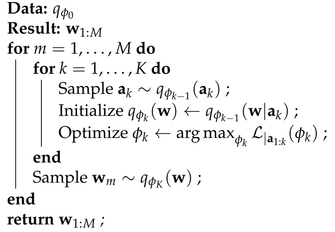 |
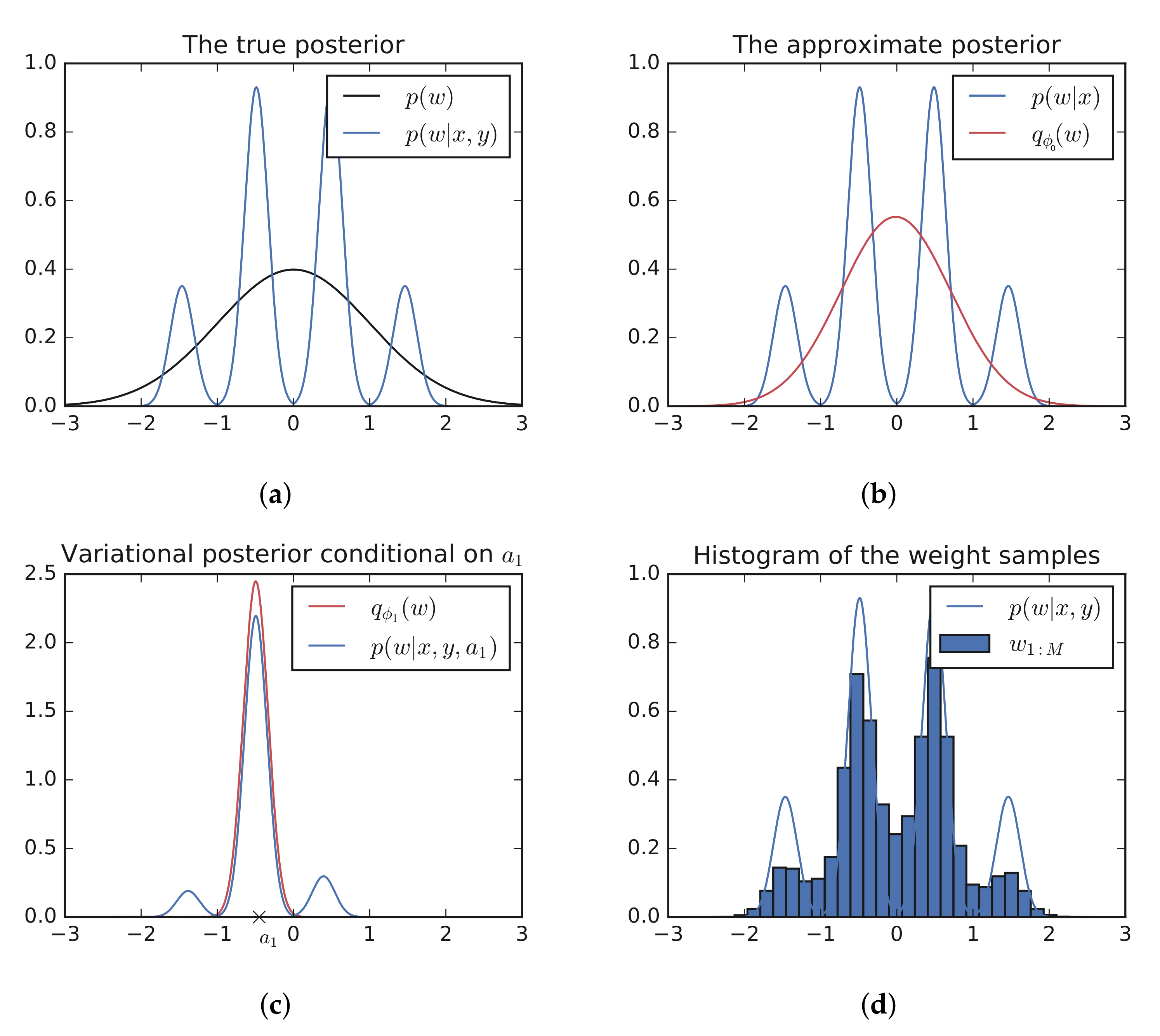
- Sample the value of using the current variational approximation and fix its value.A sample can be obtained by first sampling followed by . This is straightforward for exponential families and factorized distributions. The closed form for is provided in the Appendix A.
- Optimize the variational approximation conditional on the sampled : .This optimization is very fast in practice if is initialized using the solution from the previous iteration: . The closed form of provided in the Appendix A.
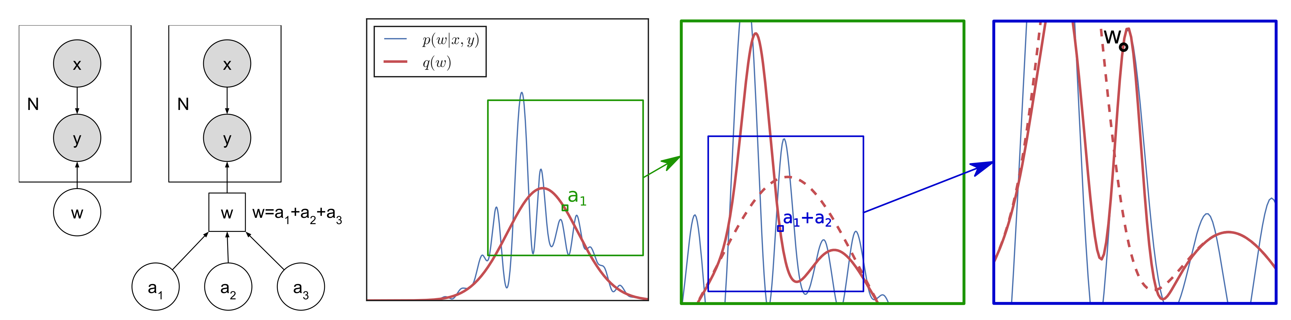
2.3. Multi-Modal Toy Example
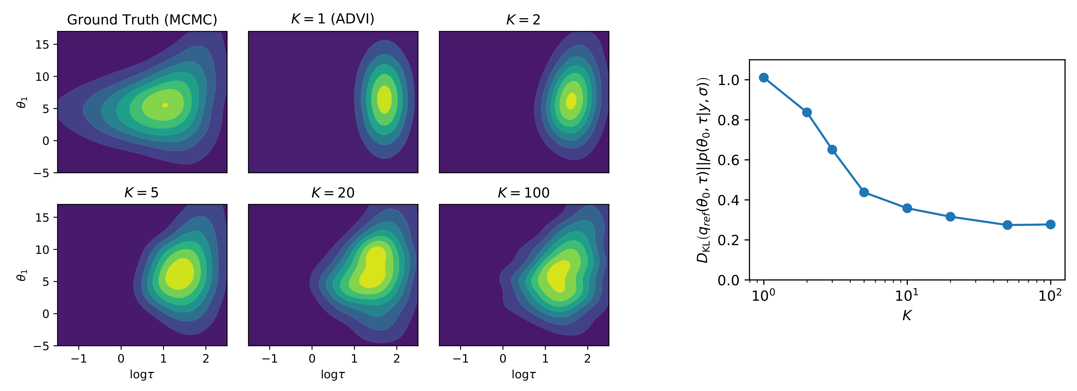
2.4. Capturing Dependencies: A Hierarchical Example
2.5. Limit as
3. Theoretical Results
3.1. Proof of
3.2. Proof of
4. Experimental Results
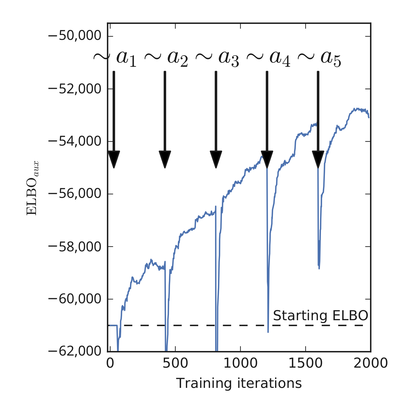
4.1. Inference in Deep Neural Networks
4.2. Computational Costs
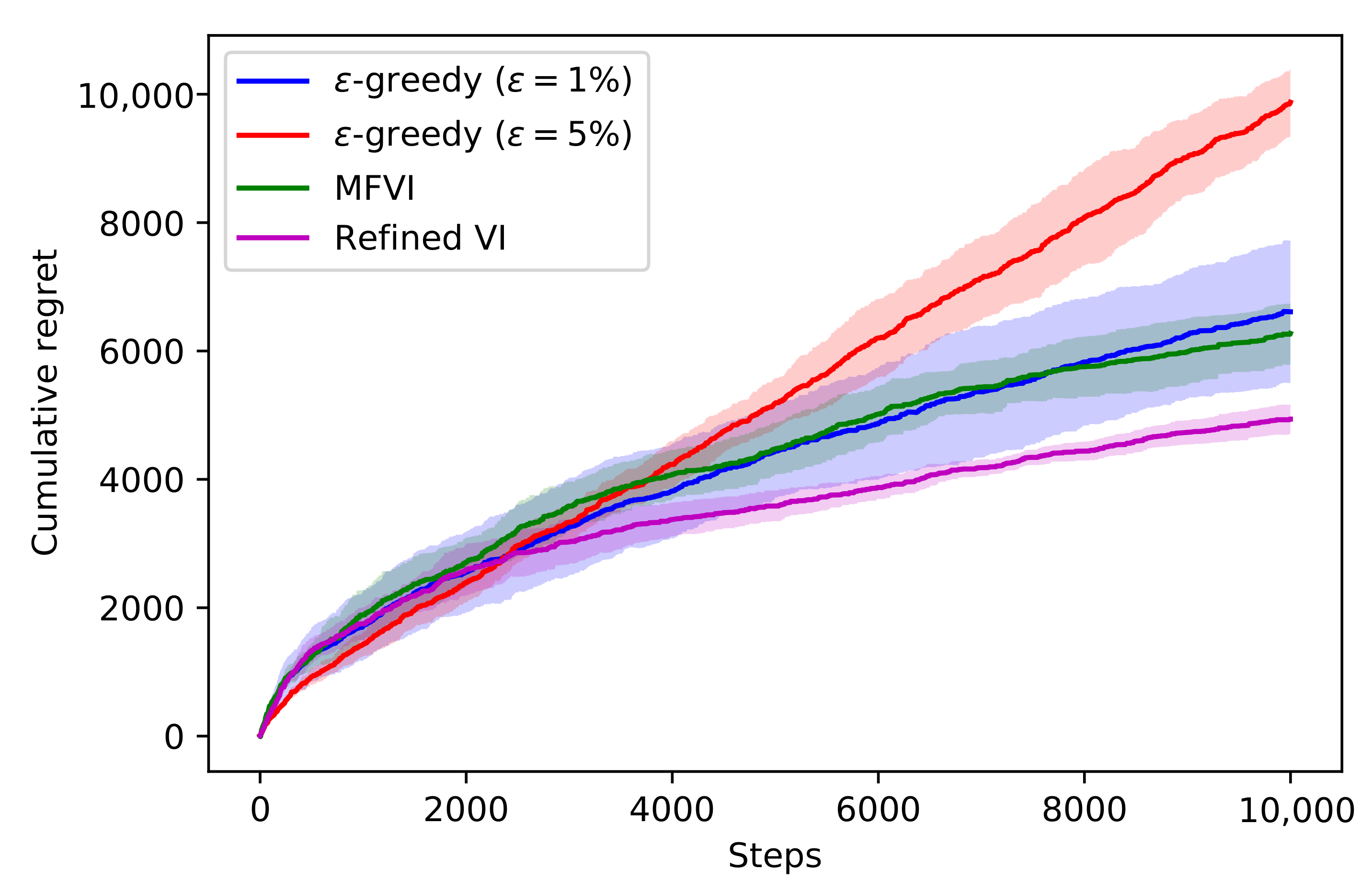
4.3. Thompson Sampling
- Sample ;
- Take action , where r is the reward that is determined by the context c, the action a taken, and the unobserved model parameters ;
- Observe reward r and update the approximate posterior .
5. Related Works
6. Conclusions
Author Contributions
Funding
Conflicts of Interest
Appendix A. Analytical Forms of qϕk−1 (ak) and qϕk−1 (w|ak)
References
- Amodei, D.; Olah, C.; Steinhardt, J.; Christiano, P.; Schulman, J.; Mané, D. Concrete problems in AI safety. arXiv 2016, arXiv:1606.06565. [Google Scholar]
- Gelman, A.; Carlin, J.B.; Stern, H.S.; Dunson, D.B.; Vehtari, A.; Rubin, D.B. Bayesian Data Analysis; Chapman and Hall/CRC: Boca Raton, FL, USA, 2013. [Google Scholar]
- Carpenter, B.; Gelman, A.; Hoffman, M.D.; Lee, D.; Goodrich, B.; Betancourt, M.; Brubaker, M.; Guo, J.; Li, P.; Riddell, A. Stan: A probabilistic programming language. J. Stat. Softw. 2017, 76, 1–32. [Google Scholar] [CrossRef] [Green Version]
- Yao, Y.; Vehtari, A.; Simpson, D.; Gelman, A. Yes, but Did It Work?: Evaluating Variational Inference. In Proceedings of the International Conference on Machine Learning, Stockholm, Sweden, 10–15 July 2018; pp. 5581–5590. [Google Scholar]
- Kucukelbir, A.; Ranganath, R.; Gelman, A.; Blei, D. Automatic variational inference in Stan. In Proceedings of the Advances in Neural Information Processing Systems, Montreal, QC, Canada, 7–12 December 2015; pp. 568–576. [Google Scholar]
- Hoffman, M.D.; Gelman, A. The No-U-Turn sampler: Adaptively setting path lengths in Hamiltonian Monte Carlo. J. Mach. Learn. Res. 2014, 15, 1593–1623. [Google Scholar]
- Salvatier, J.; Wiecki, T.V.; Fonnesbeck, C. Probabilistic programming in Python using PyMC3. PeerJ Comput. Sci. 2016, 2, e55. [Google Scholar] [CrossRef] [Green Version]
- Graves, A. Practical variational inference for neural networks. In Proceedings of the Advances in Neural Information Processing Systems, Granada, Spain, 12–14 December 2011; pp. 2348–2356. [Google Scholar]
- Blundell, C.; Cornebise, J.; Kavukcuoglu, K.; Wierstra, D. Weight uncertainty in neural network. In Proceedings of the International Conference on Machine Learning, Lille, France, 7–9 July 2015; pp. 1613–1622. [Google Scholar]
- Louizos, C.; Welling, M. Multiplicative normalizing flows for variational Bayesian neural networks. In Proceedings of the 34th International Conference on Machine Learning, Sydney, Australia, 6–11 August 2017; Volume 70, pp. 2218–2227. [Google Scholar]
- Lakshminarayanan, B.; Pritzel, A.; Blundell, C. Simple and scalable predictive uncertainty estimation using deep ensembles. In Proceedings of the Advances in Neural Information Processing Systems, Long Beach, CA, USA, 4–9 December 2017; pp. 6402–6413. [Google Scholar]
- Kingma, D.P.; Ba, J. Adam: A Method for Stochastic Optimization. arXiv 2014, arXiv:1412.6980. [Google Scholar]
- Hernández-Lobato, J.M.; Adams, R. Probabilistic backpropagation for scalable learning of Bayesian neural networks. In Proceedings of the International Conference on Machine Learning, Lille, France, 7–9 July 2015; pp. 1861–1869. [Google Scholar]
- Kingma, D.P.; Salimans, T.; Welling, M. Variational Dropout and the Local Reparameterization Trick. In Advances in Neural Information Processing Systems; MIT Press: Cambridge, MA, USA, 2015. [Google Scholar]
- LeCun, Y.; Bengio, Y. Convolutional networks for images, speech, and time series. In The Handbook of Brain Theory and Neural Networks; A Bradford Book; MIT Press: Cambridge, MA, USA, 1995. [Google Scholar]
- Wen, Y.; Vicol, P.; Ba, J.; Tran, D.; Grosse, R. Flipout: Efficient pseudo-independent weight perturbations on mini-batches. arXiv 2018, arXiv:1803.04386. [Google Scholar]
- He, K.; Zhang, X.; Ren, S.; Sun, J. Deep residual learning for image recognition. In Proceedings of the IEEE Conference on Computer Vision and Pattern Recognition, Las Vegas, NV, USA, 27–30 June 2016; pp. 770–778. [Google Scholar]
- Ovadia, Y.; Fertig, E.; Ren, J.; Nado, Z.; Sculley, D.; Nowozin, S.; Dillon, J.V.; Lakshminarayanan, B.; Snoek, J. Can You Trust Your Model’s Uncertainty? Evaluating Predictive Uncertainty Under Dataset Shift. In Proceedings of the Advances in Neural Information Processing Systems, Vancouver, BC, Canada, 8–9 December 2019. [Google Scholar]
- Ioffe, S.; Szegedy, C. Batch normalization: Accelerating deep network training by reducing internal covariate shift. arXiv 2015, arXiv:1502.03167. [Google Scholar]
- Osawa, K.; Swaroop, S.; Jain, A.; Eschenhagen, R.; Turner, R.E.; Yokota, R.; Khan, M.E. Practical Deep Learning with Bayesian Principles. In Proceedings of the Advances in Neural Information Processing Systems, Vancouver, BC, Canada, 8–14 December 2019. [Google Scholar]
- Wen, Y.; Tran, D.; Ba, J. BatchEnsemble: An Alternative Approach to Efficient Ensemble and Lifelong Learning. In Proceedings of the International Conference on Learning Representations, New Orleans, LA, USA, 6–9 May 2019. [Google Scholar]
- Thompson, W.R. On the likelihood that one unknown probability exceeds another in view of the evidence of two samples. Biometrika 1933, 25, 285–294. [Google Scholar] [CrossRef]
- Hernández-Lobato, J.M.; Requeima, J.; Pyzer-Knapp, E.O.; Aspuru-Guzik, A. Parallel and distributed Thompson sampling for large-scale accelerated exploration of chemical space. In Proceedings of the International Conference on Machine Learning, Sydney, Australia, 6–11 August 2017; pp. 1470–1479. [Google Scholar]
- Guez, A. Sample-Based Search Methods for Bayes-Adaptive Planning. Ph.D. Thesis, UCL (University College London), London, UK, 2015. [Google Scholar]
- Hinton, G.; Van Camp, D. Keeping neural networks simple by minimizing the description length of the weights. In Proceedings of the 6th Ann. ACM Conf. on Computational Learning Theory, Santa Cruz, CA, USA, 26–28 July 1993. [Google Scholar]
- Peterson, C. A mean field theory learning algorithm for neural networks. Complex Syst. 1987, 1, 995–1019. [Google Scholar]
- Kingma, D.P.; Welling, M. Auto-encoding variational Bayes. arXiv 2013, arXiv:1312.6114. [Google Scholar]
- Nguyen, C.V.; Li, Y.; Bui, T.D.; Turner, R.E. Variational continual learning. arXiv 2017, arXiv:1710.10628. [Google Scholar]
- Riquelme, C.; Tucker, G.; Snoek, J.R. Deep Bayesian Bandits Showdown. In Proceedings of the International Conference on Representation Learning, Vancouver, BC, Canada, 30 April–3 May 2018. [Google Scholar]
- Zhang, C.; Butepage, J.; Kjellstrom, H.; Mandt, S. Advances in variational inference. IEEE Trans. Pattern Anal. Mach. Intell. 2018, 41, 2008–2026. [Google Scholar] [CrossRef] [PubMed] [Green Version]
- Agakov, F.V.; Barber, D. An auxiliary variational method. In Proceedings of the International Conference on Neural Information Processing, Calcutta, India, 22–25 November 2004; pp. 561–566. [Google Scholar]
- Ranganath, R.; Tran, D.; Blei, D. Hierarchical variational models. In Proceedings of the International Conference on Machine Learning, New York, NY, USA, 20–22 June 2016; pp. 324–333. [Google Scholar]
- Salimans, T.; Kingma, D.; Welling, M. Markov chain monte carlo and variational inference: Bridging the gap. In Proceedings of the International Conference on Machine Learning, Lille, France, 7–9 July 2015; pp. 1218–1226. [Google Scholar]
- Zhang, Y.; Hernández-Lobato, J.M.; Ghahramani, Z. Ergodic measure preserving flows. arXiv 2018, arXiv:1805.10377. [Google Scholar]
- Ruiz, F.; Titsias, M. A Contrastive Divergence for Combining Variational Inference and MCMC. In Proceedings of the International Conference on Machine Learning, Long Beach, CA, USA, 9–15 June 2019; pp. 5537–5545. [Google Scholar]
- Guo, F.; Wang, X.; Fan, K.; Broderick, T.; Dunson, D.B. Boosting variational inference. arXiv 2016, arXiv:1611.05559. [Google Scholar]
- Miller, A.C.; Foti, N.J.; Adams, R.P. Variational Boosting: Iteratively Refining Posterior Approximations. In Proceedings of the International Conference on Machine Learning, Sydney, Australia, 6–11 August 2017. [Google Scholar]
- Locatello, F.; Dresdner, G.; Khanna, R.; Valera, I.; Raetsch, G. Boosting Black Box Variational Inference. In Proceedings of the Advances in Neural Information Processing Systems, Montreal, QC, Canada, 3–8 December 2018. [Google Scholar]
- Hjelm, D.; Salakhutdinov, R.R.; Cho, K.; Jojic, N.; Calhoun, V.; Chung, J. Iterative refinement of the approximate posterior for directed belief networks. In Proceedings of the Advances in Neural Information Processing Systems, Barcelona, Spain, 5–10 December 2016; pp. 4691–4699. [Google Scholar]
- Cremer, C.; Li, X.; Duvenaud, D. Inference suboptimality in variational autoencoders. arXiv 2018, arXiv:1801.03558. [Google Scholar]
- Kim, Y.; Wiseman, S.; Miller, A.C.; Sontag, D.; Rush, A.M. Semi-amortized variational autoencoders. arXiv 2018, arXiv:1802.02550. [Google Scholar]
- Marino, J.; Yue, Y.; Mandt, S. Iterative amortized inference. arXiv 2018, arXiv:1807.09356. [Google Scholar]
- Breiman, L. Bagging predictors. Mach. Learn. 1996, 24, 123–140. [Google Scholar] [CrossRef] [Green Version]


| Deep Ensemble | MNF | VI | Refined VI (This Work) | |||
|---|---|---|---|---|---|---|
| MLL | MLL | MLL | ELBO | MLL | ||
| Boston | −9.136 ± 5.719 | −2.920 ± 0.133 | −2.874 ± 0.151 | −668.2 ± 7.6 | −2.851 ± 0.185 | −630.3 ± 7.7 |
| Concrete | −4.062 ± 0.130 | −3.202 ± 0.055 | −3.138 ± 0.063 | −3248.1 ± 68.5 | −3.131 ± 0.062 | −3071.1 ± 64.0 |
| Naval | 3.995 ± 0.013 | 3.473 ± 0.007 | 5.969 ± 0.245 | 53,440.7 ± 2047.3 | 6.128 ± 0.171 | 54,882.6 ± 1228.3 |
| Energy | −0.666 ± 0.058 | −0.756 ± 0.054 | −0.749 ± 0.068 | −1296.7 ± 66.3 | −0.707 ± 0.094 | −1192.3 ± 62.0 |
| Yacht | −0.984 ± 0.104 | −1.339 ± 0.170 | −1.749 ± 0.232 | −928.7 ± 112.9 | −1.626 ± 0.231 | −790.0 ± 84.7 |
| Kin8nm | 1.135 ± 0.012 | 1.125 ± 0.022 | 1.066 ± 0.019 | 6071.2 ± 61.7 | 1.069 ± 0.018 | 6172.7 ± 67.6 |
| Power | −3.935 ± 0.140 | −2.835 ± 0.033 | −2.826 ± 0.020 | −22,496.5 ± 130.4 | −2.820 ± 0.024 | −22,368.9 ± 85.3 |
| Protein | −3.687 ± 0.013 | −2.928 ± 0.0 | −2.926 ± 0.010 | −108,806.007 ± 174.5 | −2.923 ± 0.009 | −108,597.5 ± 158.4 |
| Wine | −0.968 ± 0.079 | −0.963 ± 0.027 | −0.973 ± 0.054 | −1346.1 ± 18.0 | −0.968 ± 0.056 | −1311.8 ± 17.4 |
| Deep Ensemble | MNF | VI | Refined VI (This Work) | |||
|---|---|---|---|---|---|---|
| MLL & Acc | MLL & Acc | MLL & Acc | ELBO | MLL & Acc | ||
| mnist | −0.017 ± 0.001 | −0.034 ± 0.002 | −0.032 ± 0.001 | −7618.5 ± 47.5 | −0.025 ± 0.001 | −6310.8 ± 42.3 |
| 99.4% ± 0.0 | 99.1% ± 0.1 | 99.1% ± 0.1 | 99.2% ± 0.0 | |||
| fashion_mnist | −0.201 ± 0.002 | −0.255 ± 0.004 | −0.255 ± 0.003 | −22,830.3 ± 232.6 | −0.241 ± 0.004 | −20,438.9 ± 79.6 |
| 93.1% ± 0.1 | 90.7% ± 0.2 | 90.7% ± 0.1 | 91.3% ± 0.2 | |||
| cifar10 | −0.791 ± 0.009 | −0.795 ± 0.013 | −0.815 ± 0.004 | −57,257.8 ± 299.5 | −0.768 ± 0.007 | −50,989.2 ± 238.9 |
| 76.3% ± 0.3 | 72.8% ± 0.6 | 72.3% ± 0.5 | 73.5% ± 0.5 | |||
| Deep Ensemble | VI | Refined VI (This Work) | ||||
|---|---|---|---|---|---|---|
| MLL | Acc | MLL | Acc | MLL | Acc | |
| ResNet | −0.698 | 82.7% | −0.795 | 72.6% | −0.696 | 75.5% |
| ResNet + BatchNorm | −0.561 | 83.6% | −0.672 | 77.6% | −0.593 | 79.7% |
| ResNet Hybrid | −0.698 | 82.7% | −0.465 | 84.2% | −0.432 | 85.8% |
| ResNet Hybrid + BatchNorm | −0.561 | 83.6% | −0.465 | 84.0% | −0.423 | 85.6% |
Publisher’s Note: MDPI stays neutral with regard to jurisdictional claims in published maps and institutional affiliations. |
© 2021 by the authors. Licensee MDPI, Basel, Switzerland. This article is an open access article distributed under the terms and conditions of the Creative Commons Attribution (CC BY) license (https://creativecommons.org/licenses/by/4.0/).
Share and Cite
Havasi, M.; Snoek, J.; Tran, D.; Gordon, J.; Hernández-Lobato, J.M. Sampling the Variational Posterior with Local Refinement. Entropy 2021, 23, 1475. https://doi.org/10.3390/e23111475
Havasi M, Snoek J, Tran D, Gordon J, Hernández-Lobato JM. Sampling the Variational Posterior with Local Refinement. Entropy. 2021; 23(11):1475. https://doi.org/10.3390/e23111475
Chicago/Turabian StyleHavasi, Marton, Jasper Snoek, Dustin Tran, Jonathan Gordon, and José Miguel Hernández-Lobato. 2021. "Sampling the Variational Posterior with Local Refinement" Entropy 23, no. 11: 1475. https://doi.org/10.3390/e23111475
APA StyleHavasi, M., Snoek, J., Tran, D., Gordon, J., & Hernández-Lobato, J. M. (2021). Sampling the Variational Posterior with Local Refinement. Entropy, 23(11), 1475. https://doi.org/10.3390/e23111475