
Ultra-Low-Power, High-Accuracy 434 MHz Indoor Positioning System for Smart Homes Leveraging Machine Learning Models

 , , , ,
Abstract
:
1. Introduction
2. Materials and Methods
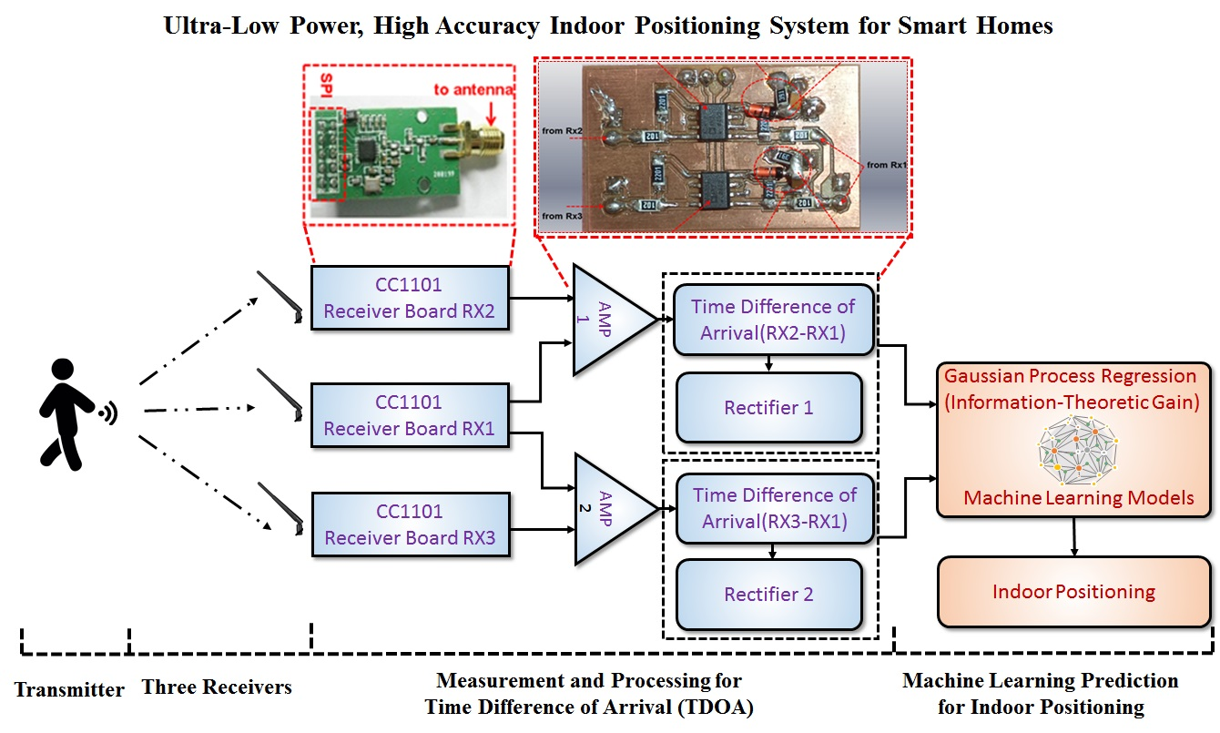
3. The Proposed Indoor Positioning System
3.1. Proposed System Architecture and Description
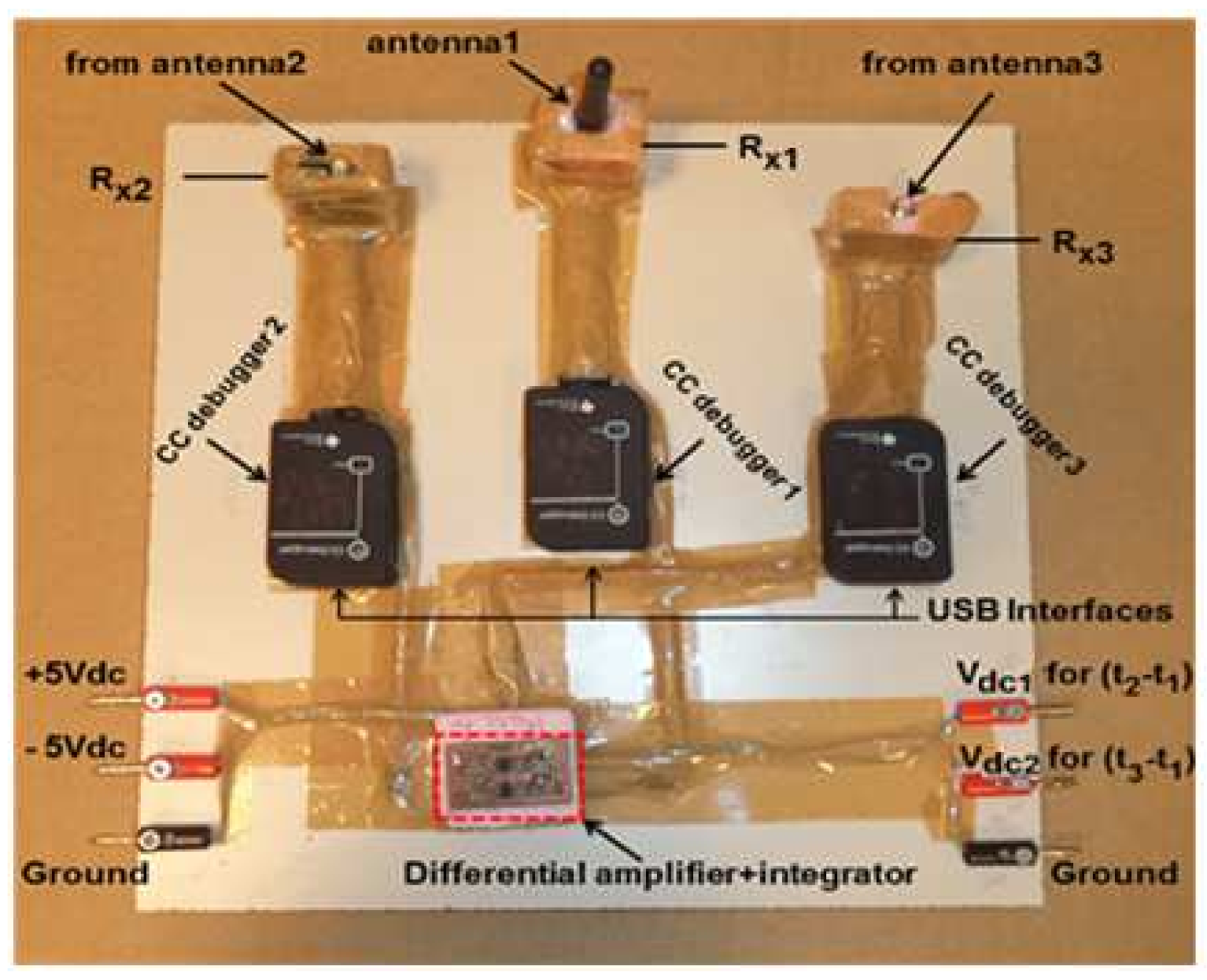
3.2. Proposed System Design, Implementation and Integration
4. Results and Discussion
5. Conclusions
Author Contributions
Funding
Data Availability Statement
Conflicts of Interest
References
- Sakpere, W.; Oshin, M.A.; Mlitwa, N. A State-of-the-Art Survey of Indoor Positioning and Navigation Systems and Technologies. S. Afr. Comput. J. 2017, 29, 145–197. [Google Scholar] [CrossRef] [Green Version]
- Turgut, Z.; Aydin, G.Z.G.; Sertbas, A. Indoor Localization Techniques for Smart Building Environment. Procedia Comput. Sci. 2016, 83, 1176–1181. [Google Scholar] [CrossRef] [Green Version]
- Yiu, S.; Dashti, M.; Claussen, H.; Perez-Cruz, F. Wireless RSSI Fingerprinting Localization. Signal Process. 2017, 131, 235–244. [Google Scholar] [CrossRef]
- Mahani, E.A.; Taheri, M.; Dastgheibifard, G.H. A Novel Descent Method of Localization in Wireless Sensor Networks. In Proceedings of the 2019 27th Iranian Conference on Electrical Engineering (ICEE), Yazd, Iran, 30 April–2 May 2019; pp. 2057–2061. [Google Scholar]
- Khan, M.A.; Saeed, N.; Ahmad, A.W.; Lee, C. Location Awareness in 5G Networks Using RSS Measurements for Public Safety Applications. IEEE Access 2017, 5, 21753–21762. [Google Scholar] [CrossRef]
- Ahmad, I.; Asif, R.; Abd-Alhameed, R.A.; Alhassan, H.; Elmegri, F.; Noras, J.M.; See, C.H.; Obidat, H.; Shuaieb, W.; Riberio, J.C.; et al. Current Technologies and Location Based Services. In Proceedings of the 2017 Internet Technologies and Applications (ITA), Wrexham, UK, 12–15 September 2017; pp. 299–304. [Google Scholar]
- Batistić, L.; Tomic, M. Overview of Indoor Positioning System Technologies. In Proceedings of the 2018 41st International Convention on Information and Communication Technology, Electronics and Microelectronics (MIPRO), Opatija, Croatia, 21–25 May 2018; pp. 0473–0478. [Google Scholar]
- Guan, Z.X.; Zhang, B.H.; Zhang, Y.; Zhang, S.; Wang, F.F. Delaunay Triangulation Based Localization Scheme. In Proceedings of the 2017 29th Chinese Control And Decision Conference (CCDC), Chongqing, China, 28–30 May 2017; pp. 2627–2631. [Google Scholar]
- Wang, Z.F.; Zhang, H.; Lu, T.T.; Gulliver, T.A. Cooperative RSS-Based Localization in Wireless Sensor Networks Using Relative Error Estimation and Semi definite Programming. IEEE Trans. Veh. Technol. 2019, 68, 483–497. [Google Scholar] [CrossRef]
- Tomic, S.; Beko, M.; Dinis, R. RSS-Based Localization in Wireless Sensor Networks Using Convex Relaxation: Non-cooperative and Cooperative Schemes. IEEE Trans. Veh. Technol. 2015, 64, 2037–2050. [Google Scholar] [CrossRef] [Green Version]
- Bouchard, K.; Ramezani, R.; Naeim, A. Features Based Proximity Localization with Bluetooth Emitters. In Proceedings of the 2016 IEEE 7th Annual Ubiquitous Computing, Electronics & Mobile Communication Conference (UEMCON), New York, NY, USA, 20–22 October 2016; pp. 1–5. [Google Scholar]
- Maletic, N.; Sark, V.; Ehrig, M.; Gutiérrez, J.; Grass, E. Experimental Evaluation of Round-Trip ToF-based Localization in the 60 GHz Band. In Proceedings of the 2019 International Conference on Indoor Positioning and Indoor Navigation (IPIN), Pisa, Italy, 30 September–3 October 2019; pp. 1–6. [Google Scholar]
- Hou, Y.; Yang, X.; Abbasi, Q. Efficient AoA-Based Wireless Indoor Localization for Hospital Outpatients Using Mobile Devices. Sensors 2018, 18, 3698. [Google Scholar] [CrossRef] [PubMed] [Green Version]
- Menta, E.Y.; Malm, N.; Jäntti, R.; Ruttik, K.; Costa, M.; Leppänen, K. On the Performance of AoA–Based Localization in 5G Ultra–Dense Networks. IEEE Access 2019, 7, 33870–33880. [Google Scholar] [CrossRef]
- Kim, S.; Park, S.; Ji, H.; Shim, B. AOA-TOA Based Localization for 5G Cell-less Communications. In Proceedings of the 2017 23rd Asia-Pacific Conference on Communications (APCC), Perth, WA, Australia, 11–13 December 2017; pp. 1–6. [Google Scholar]
- Azmi, N.A.; Samsul, S.; Yamada, Y.; MohdYakub, M.F.; Mohd Ismail, M.I.; Dziyauddin, R.A. A Survey of Localization using RSSI and TDOA Techniques in Wireless Sensor Network: System Architecture. In Proceedings of the 2018 2nd International Conference on Telematics and Future Generation Networks (TAFGEN), Kuching, Malaysia, 24–26 July 2018; pp. 131–136. [Google Scholar]
- Zhang, L.; Chen, M.; Wang, X.; Wang, Z. TOA Estimation of Chirp Signal in Dense Multipath Environment for Low-Cost Acoustic Ranging. IEEE Trans. Instrum. Meas. 2019, 68, 355–367. [Google Scholar] [CrossRef]
- Segura, M.; Mut, V.; Sisterna, C. Ultra wideband Indoor Navigation System. IET Radar Sonar Navig. 2012, 6, 402–411. [Google Scholar] [CrossRef]
- Alarifi, A.; Al-Salman, A.; Alsaleh, M.; Alnafessah, A.; Al-Hadhrami, S.; Al-Ammar, M.A.; Al-Khalifa, H.S. Ultra Wideband Indoor Positioning Technologies: Analysis and Recent Advances. Sensors 2016, 16, 707. [Google Scholar] [CrossRef] [PubMed]
- Yu, Y.; Chen, R.; Liu, Z.; Guo, G.; Chen, L. Wi-Fi Fine Time Measurement: Data Analysis and Processing for Indoor Localization. J. Navig. 2020, 73, 1–23. [Google Scholar] [CrossRef]
- Ayyalasomayajula, R.; Vasisht, D.; Bharadia, D. BLoc: CSI-based Accurate Localization for BLE Tags. In Proceedings of the 14th International Conference on Emerging Networking EXperiments and Technologies, 4 December 2018; pp. 126–138. [Google Scholar]
- Wu, Z.F.; Jiang, L.; Jiang, Z.Z.; Chen, B.; Liu, K.; Xuan, Q.; Xiang, Y. Accurate Indoor Localization Based on CSI and Visibility Graph. Sensors 2018, 18, 2549. [Google Scholar] [CrossRef] [PubMed] [Green Version]
- Wang, X.; Zhang, C.; Liu, F.; Dong, Y.; Xu, X. Exponentially Weighted Particle Filter for Simultaneous Localization and Mapping Based on Magnetic Field Measurements. IEEE Trans. Instrum. Meas. 2017, 66, 1658–1667. [Google Scholar] [CrossRef]
- Obeidat, H.; Shuaieb, W.; Obeidat, O.; Abd-Alhameed, R. A Review of Indoor Localization Techniques and Wireless Technologies. Wirel. Pers. Commun. 2021, 119, 289–327. [Google Scholar] [CrossRef]
- Li, X.; Deng, Z.D.; Rauchenstein, L.T.; Carlson, T.J. Contributed review: Source-localization Algorithms and Applications Using Time of Arrival and Time Difference of Arrival Measurements. Rev. Sci. Instrum. 2016, 87, 041502. [Google Scholar] [CrossRef]
- Zafari, F.; Gkelias, A.; Leung, K.K. A Survey of Indoor Localization Systems and Technologies. IEEE Commun. Surv. Tutor. 2019, 21, 2568–2599. [Google Scholar] [CrossRef] [Green Version]
- Yang, B. Different Sensor Placement Strategies for TDOA Based Localization. In Proceedings of the 2007 IEEE International Conference on Acoustics, Speech and Signal Processing—ICASSP ’07, Honolulu, HI, USA, 15–20 April 2007; pp. 1093–1096. [Google Scholar]
- Dalveren, Y.; Kara, A. Comparative Analysis of TDOA-based Localization Methods in the Presence of Sensor Position Errors. In Proceedings of the 2017 4th International Conference on Control, Decision and Information Technologies (CoDIT), Barcelona, Spain, 5–7 April 2017; pp. 0556–0560. [Google Scholar]
- Kim, S.; Chong, J.-W. An Efficient TDOA-Based Localization Algorithm without Synchronization between Base Stations. Int. J. Distrib. Sensor Netw. 2015. [Google Scholar] [CrossRef] [Green Version]
- Yoon, J.-Y.; Kim, J.-W.; Lee, W.-Y.; Eom, D.-S. A TDOA-based Localization Using Precise Time-synchronization. In Proceedings of the 2012 14th International Conference on Advanced Communication Technology (ICACT), PyeongChang, Korea, 19–22 February 2012; pp. 1266–1271. [Google Scholar]
- Xu, B.; Sun, G.; Yu, R.; Yang, Z. High-Accuracy TDOA-Based Localization without Time Synchronization. IEEE Trans. Parallel Distrib. Syst. 2013, 24, 1567–1576. [Google Scholar] [CrossRef] [Green Version]
- Kietlinski-Zaleski, J.; Yamazato, T.; Katayama, M. TDOA UWB Positioning with Three Receivers Using Known Indoor Features. IEICE 2010, 1–4. [Google Scholar] [CrossRef]
- Liu, F.; Chen, H.; Zhang, L.; Xie, L. Time-Difference-of-Arrival-Based Localization Methods of Underwater Mobile Nodes Using Multiple Surface Beacons. IEEE Access 2021, 9, 31712–31725. [Google Scholar] [CrossRef]
- Díez-González, J.; Álvarez, R.; Sánchez-González, L.; Fernández-Robles, L.; Pérez, H.; Castejón-Limas, M. 3D TDOA Problem Solution with Four Receiving Nodes. Sensors 2019, 19, 2892. [Google Scholar] [CrossRef] [Green Version]
- Cheng, Y.; Zhou, T. UWB Indoor Positioning Algorithm Based on TDOA Technology. In Proceedings of the 2019 10th International Conference on Information Technology in Medicine and Education (ITME), Qingdao, China, 23–25 August 2019; pp. 777–782. [Google Scholar]
- Li, S.H.; Hedley, M.; Bengston, K.; Johnson, M.; Humphrey, D.; Kajan, A.; Bhaska, N. TDOA-based Passive Localization of Standard WiFi Devices. In Proceedings of the 2018 Ubiquitous Positioning, Indoor Navigation and Location-Based Services (UPINLBS), Wuhan, China, 22–23 March 2018; pp. 1–5. [Google Scholar]
- Lee, D.; Shim, Y.; Kim, M.; Moon, Y. Hybrid Positioning System for Improving Location Recognition Performance in Offshore Plant Environment. In Proceedings of the 2018 International Conference on Information Networking (ICOIN), Chiang Mai, Thailand, 10–12 January 2018; pp. 891–893. [Google Scholar]
- Yang, K.; An, J.; Bu, X.; Sun, G. Constrained Total Least Squares Location Algorithm Using Time-difference-of-arrival Measurements. IEEE Trans. Veh. Technol. 2010, 59, 1558–1562. [Google Scholar] [CrossRef]
- Texas Instruments CC1101. Available online: http://www.ti.com/lit/ds/symlink/cc1101.pdf (accessed on 9 August 2018).
- CC Debugger User Guide. Available online: http://www.ti.com/lit/ug/swru197h/swru197h.pdf (accessed on 9 August 2018).
- He, J.; So, H.C. A Hybrid TDOA-Fingerprinting-Based Localization System for LTE Network. IEEE Sens. J. 2020, 20, 13653–13665. [Google Scholar] [CrossRef]
- Ali, M.U.; Hur, S.; Park, Y. Wi-Fi-Based Effortless Indoor Positioning System Using IoT Sensors. Sensors 2019, 19, 1496. [Google Scholar] [CrossRef] [PubMed] [Green Version]
- Lu, T.-T.; Yeh, S.-C.; Wu, S.-H. Actualizing Real-time Indoor Positioning Systems Using Plane Models. Int. J. Commun. Syst. 2016, 29, 874–892. [Google Scholar] [CrossRef]
- Chabbar, H.; Chami, M. Indoor Localization Using Wi-Fi Method Based on Fingerprinting Technique. In Proceedings of the 2017 International Conference on Wireless Technologies, Embedded and Intelligent Systems (WITS), Fez, Morocco, 19–20 April 2017; pp. 1–5. [Google Scholar]
- Ma, Y.-W.; Chen, J.-L.; Chang, F.-S.; Tang, C.-L. Novel Fingerprinting Mechanisms for Indoor Positioning. Int. J. Commun. Syst. 2016, 29, 638–656. [Google Scholar] [CrossRef]
- Lallement, G.; Abouzeid, F.; Daveau, J.-M.; Roche, P.; Autran, J.-L. A 1.1-pJ/cycle, 20-MHz, 0.42-V Temperature Compensated ARM Cortex-M0+ SoC with Adaptive Selfbody-biasing in FD-SOI. IEEE Solid-State Circuits Lett. 2018, 1, 174–177. [Google Scholar] [CrossRef]


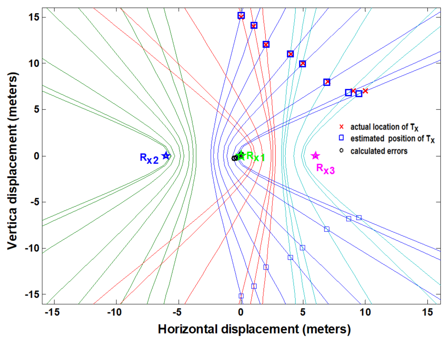
| Tx Position (x,y) | Vdc1 (mV) (d2-d1) | Vdc2 (mV) (d3-d1) |
|---|---|---|
| (0,15) | 115 | 116 |
| (1,14) | 162 | 83 |
| (2,12) | 226 | 48 |
| (4,11) | 316 | −52.5 |
| (5,10) | 369 | −113 |
| (7,8) | 463 | −257 |
| (9,7) | 515 | −378 |
| (10,7) | 526 | −414 |
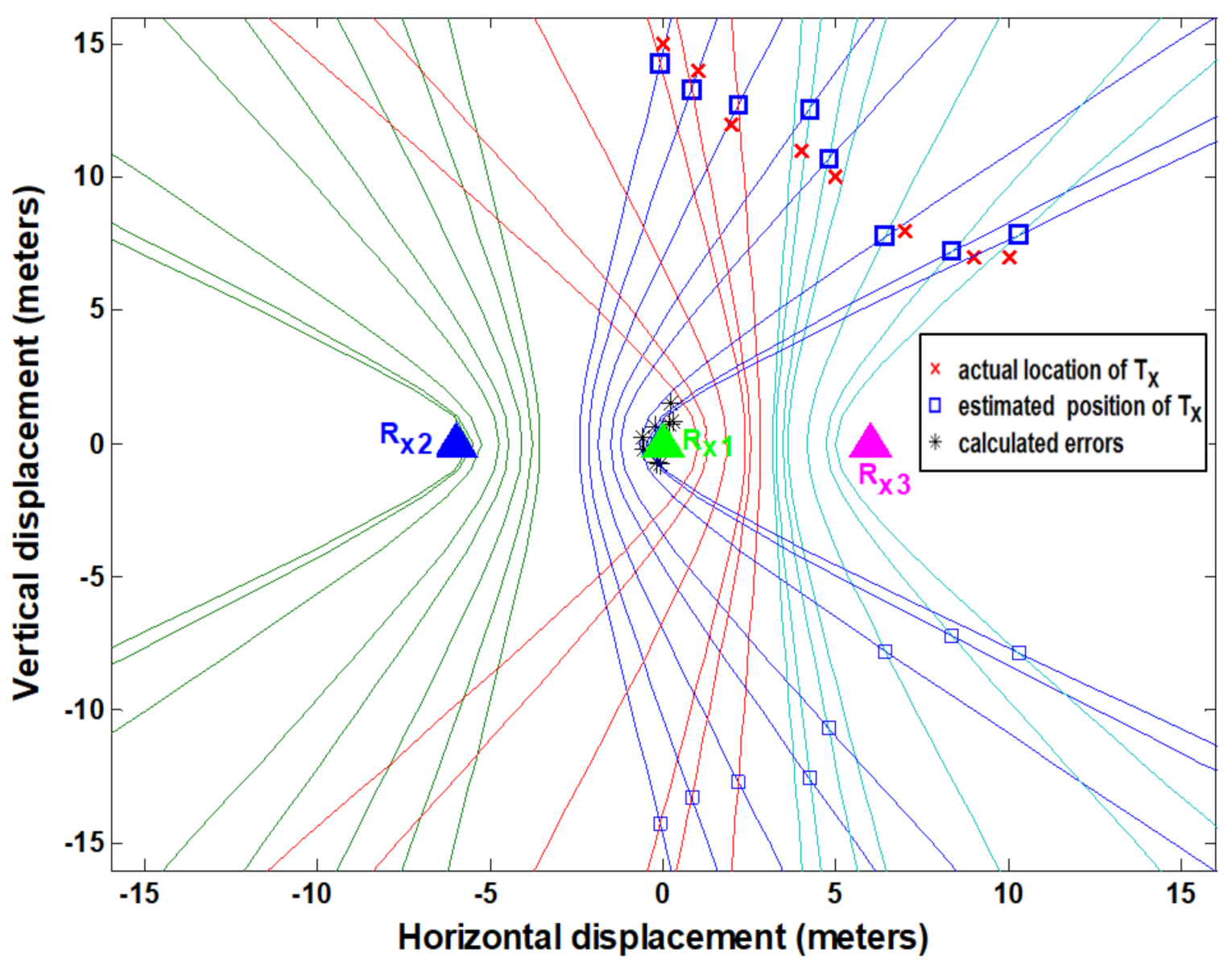
| Tx Position (x,y) | Vdc1 (mV) (d2-d1) | Vdc2 (mV) (d3-d1) |
|---|---|---|
| (0,15) | 123.5 | 131 |
| (1,14) | 170 | 100 |
| (2,12) | 233 | 40 |
| (4,11) | 310 | −60.5 |
| (5,10) | 365 | −100 |
| (7,8) | 480 | −242 |
| (9,7) | 528 | −363 |
| (10,7) | 540 | −420 |
| Machine Learning Algorithm | LOS Error (m) | NLOS Error (m) |
|---|---|---|
| Total Linear Regression | 0.80 | 1.50 |
| Gaussian Process Regression | 0.68 | 1.08 |
| Support Vector Machine (SVM) | 0.89 | 1.63 |
| Boosted Trees Ensemble | 6.93 | 7.31 |
| Bagged Trees Ensemble | 6.95 | 7.20 |
| IPS Ref. | Tech. | Accuracy | Advantage | Disadvantage |
|---|---|---|---|---|
| [13] | Angle of Arrival (AOA) | 2.5 m | Employs two access-points for positioning | Infrastructure cost would be much higher. Mainly for the line of sight (LOS)-dominating environments. |
| [41] | Time Difference of Arrival (TDOA) | ≤2 m | Improvd accuracy of sub-meter level | Two-step algorithm which require additional computing |
| [42] | Received Signal Strength Indication (RSSI) | 2 m | Automatic generation and calibration of the fingerprinting database | Accuracy dependent on path loss parameters |
| [43] | Plane model position | 3 m | Reduced computing complexity | The variations in signal strength due to obstacles were not considered. |
| [44] | RSSI | 2 m | Simple algorithm | Low localization range |
| [45] | RSSI | 1.18 | Improved positioning accuracy | The accuracy is affected by received signal variations |
| Proposed Indoor Positioning System (IPS) | TDOA | 0.68 m for LOS 1.08 m for non-line of sight (NLOS) | Simple design with good accuracy and low DC power. Dual functionality of localization and telemetry. | Lower accuracy for NLOS environment |
Publisher’s Note: MDPI stays neutral with regard to jurisdictional claims in published maps and institutional affiliations. |
© 2021 by the authors. Licensee MDPI, Basel, Switzerland. This article is an open access article distributed under the terms and conditions of the Creative Commons Attribution (CC BY) license (https://creativecommons.org/licenses/by/4.0/).
Share and Cite
Nawaz, H.; Tahir, A.; Ahmed, N.; Fayyaz, U.U.; Mahmood, T.; Jaleel, A.; Gogate, M.; Dashtipour, K.; Masud, U.; Abbasi, Q. Ultra-Low-Power, High-Accuracy 434 MHz Indoor Positioning System for Smart Homes Leveraging Machine Learning Models. Entropy 2021, 23, 1401. https://doi.org/10.3390/e23111401
Nawaz H, Tahir A, Ahmed N, Fayyaz UU, Mahmood T, Jaleel A, Gogate M, Dashtipour K, Masud U, Abbasi Q. Ultra-Low-Power, High-Accuracy 434 MHz Indoor Positioning System for Smart Homes Leveraging Machine Learning Models. Entropy. 2021; 23(11):1401. https://doi.org/10.3390/e23111401
Chicago/Turabian StyleNawaz, Haq, Ahsen Tahir, Nauman Ahmed, Ubaid U. Fayyaz, Tayyeb Mahmood, Abdul Jaleel, Mandar Gogate, Kia Dashtipour, Usman Masud, and Qammer Abbasi. 2021. "Ultra-Low-Power, High-Accuracy 434 MHz Indoor Positioning System for Smart Homes Leveraging Machine Learning Models" Entropy 23, no. 11: 1401. https://doi.org/10.3390/e23111401
APA StyleNawaz, H., Tahir, A., Ahmed, N., Fayyaz, U. U., Mahmood, T., Jaleel, A., Gogate, M., Dashtipour, K., Masud, U., & Abbasi, Q. (2021). Ultra-Low-Power, High-Accuracy 434 MHz Indoor Positioning System for Smart Homes Leveraging Machine Learning Models. Entropy, 23(11), 1401. https://doi.org/10.3390/e23111401