
A General Rate-Distortion Optimization Method for Block Compressed Sensing of Images

Abstract
:1. Introduction
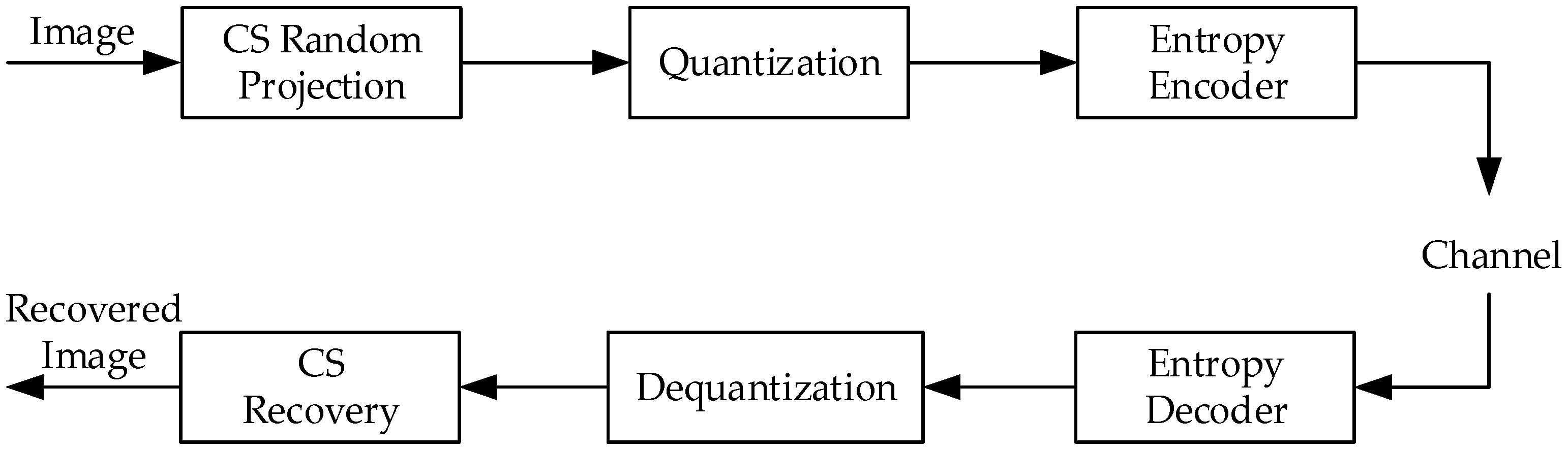
2. Problem Statement
3. Bit-Rate Model
3.1. Generalized Gaussian Distribution Model of the Quantized CS Measurements
3.2. Average Codeword Length Estimation Model
4. Optimal Bit-Depth Model
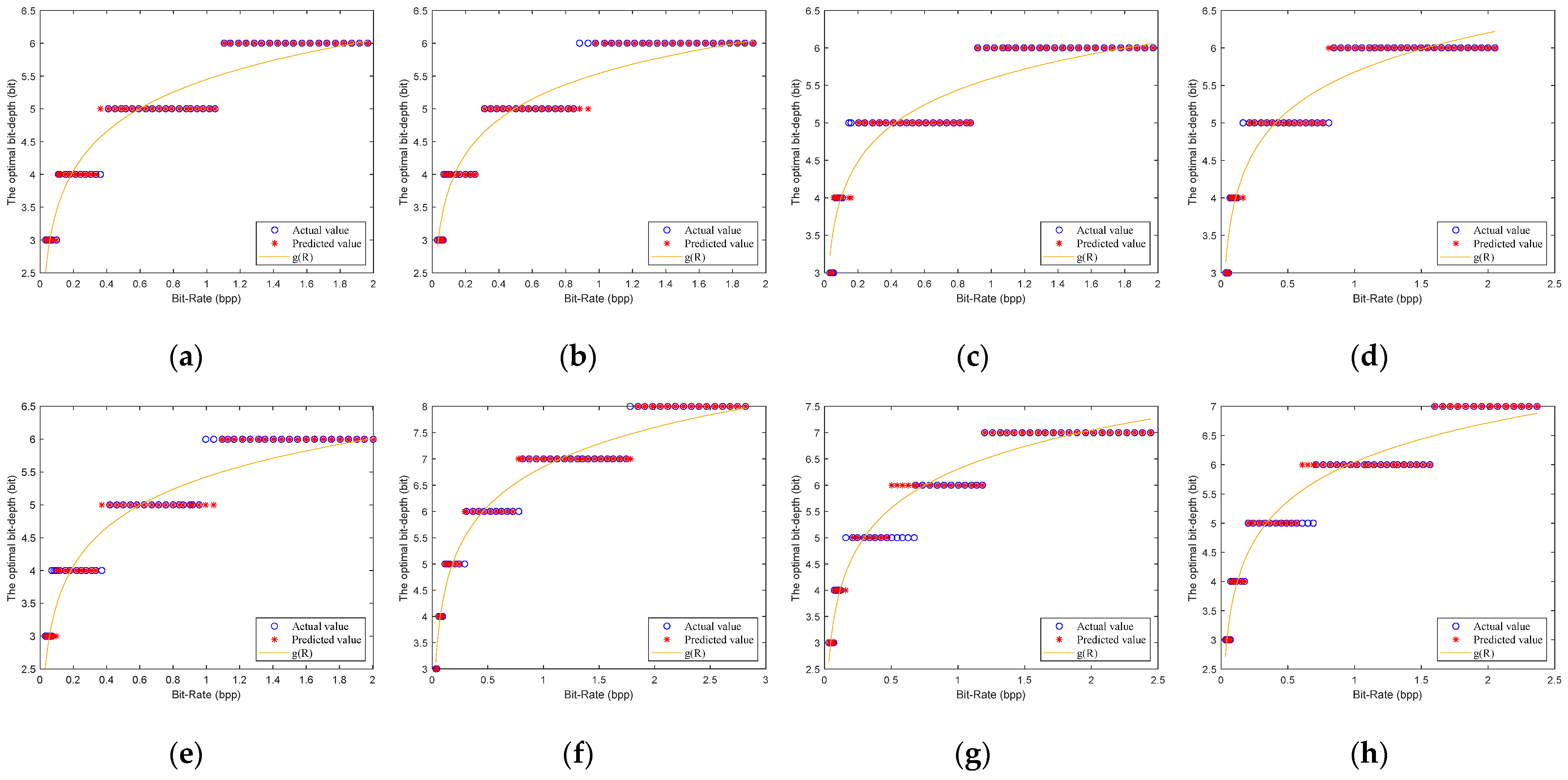
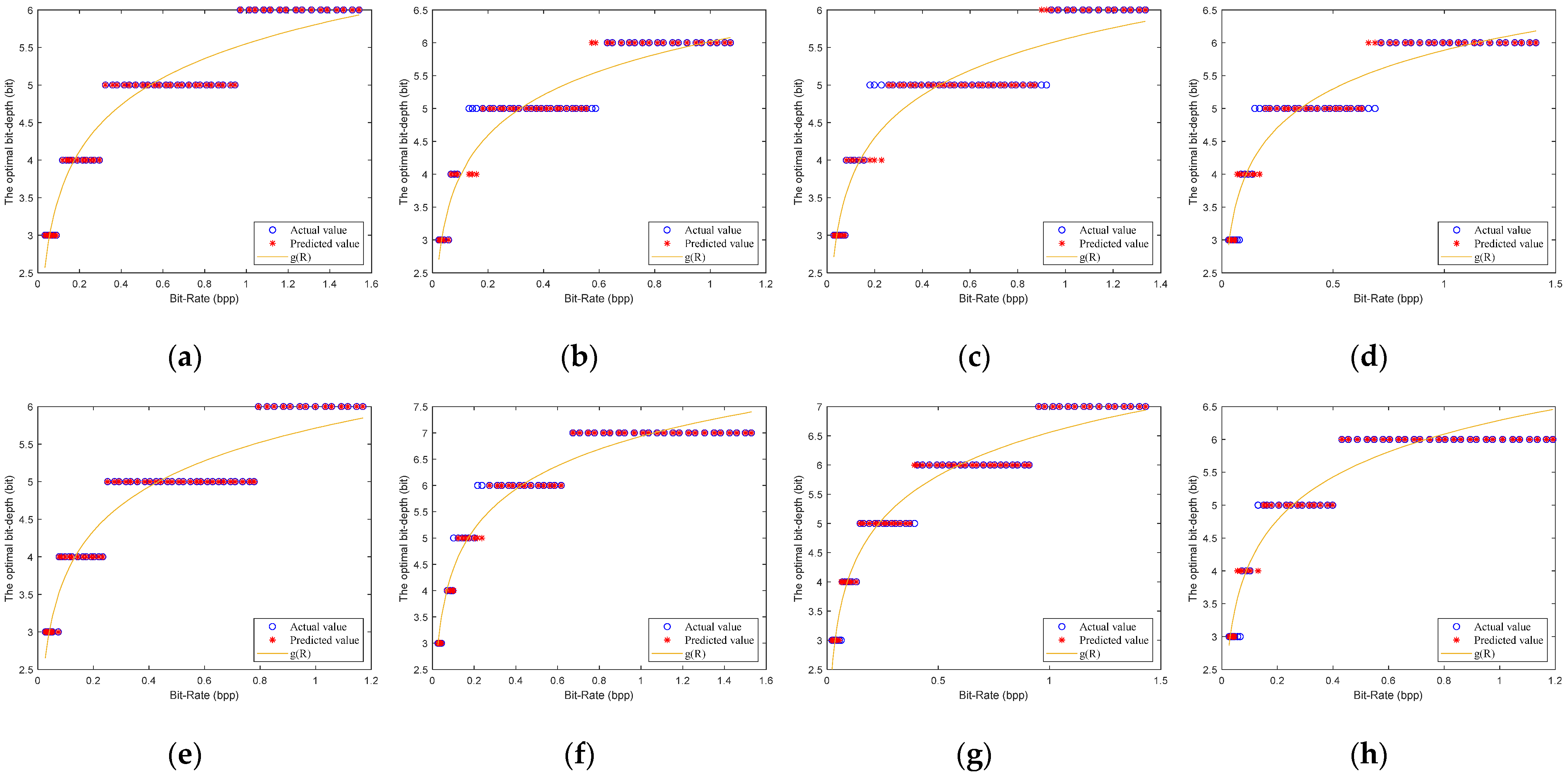
4.1. Function Mapping Relationship between Optimal Bit-Depth and Bit-Rate
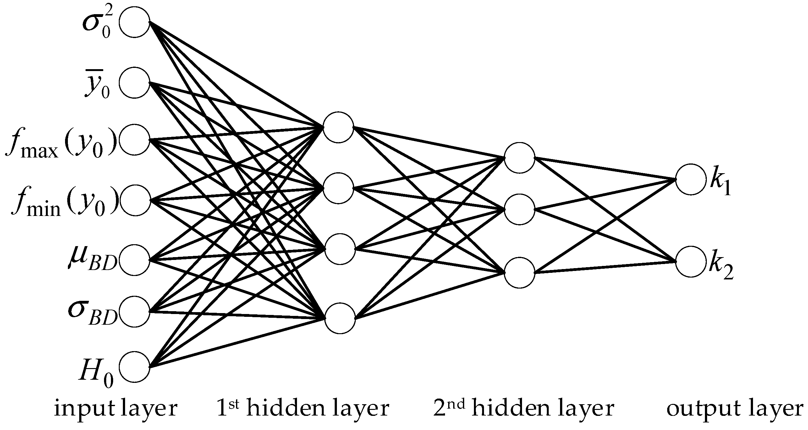
4.2. Model Parameter Estimation Based on Neural Network
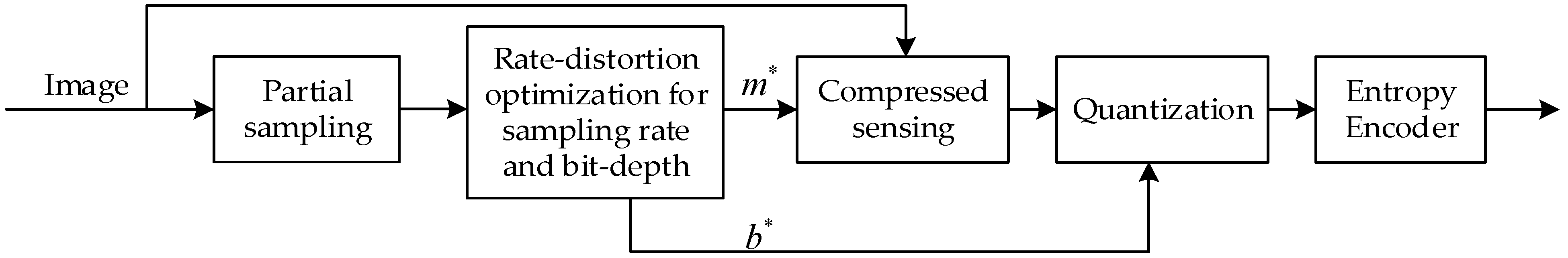
5. A General Rate-Distortion Optimization Method for Sampling Rate and Bit-Depth
5.1. Sampling Rate Modification
5.1.1. Average Codeword Length Boundary
5.1.2. Sampling Rate Boundary
5.2. Rate-Distortion Optimization Algorithm
5.3. Computational Complexity Analysis
6. Experimental Results
6.1. Model Parameters Estimation
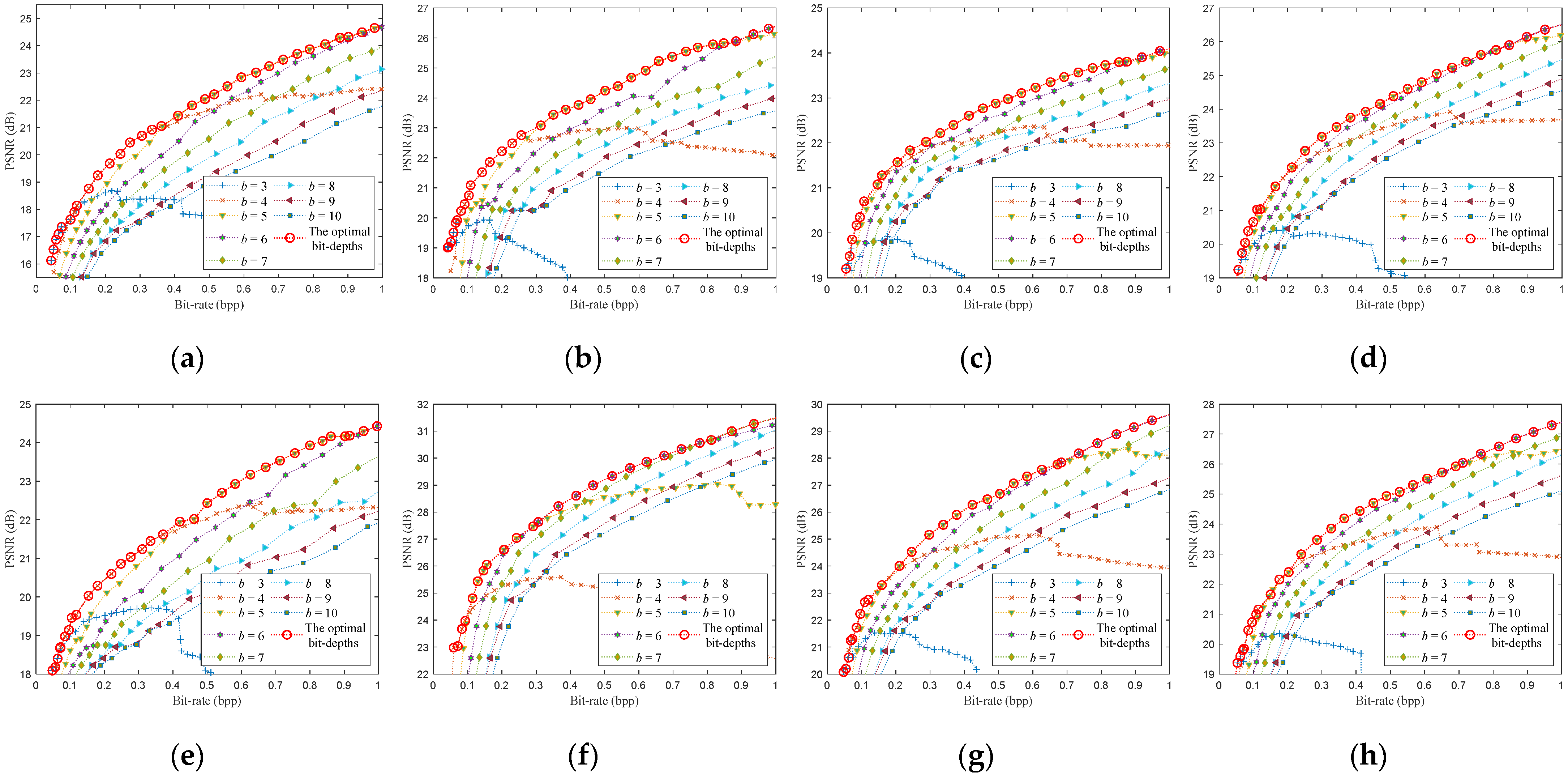
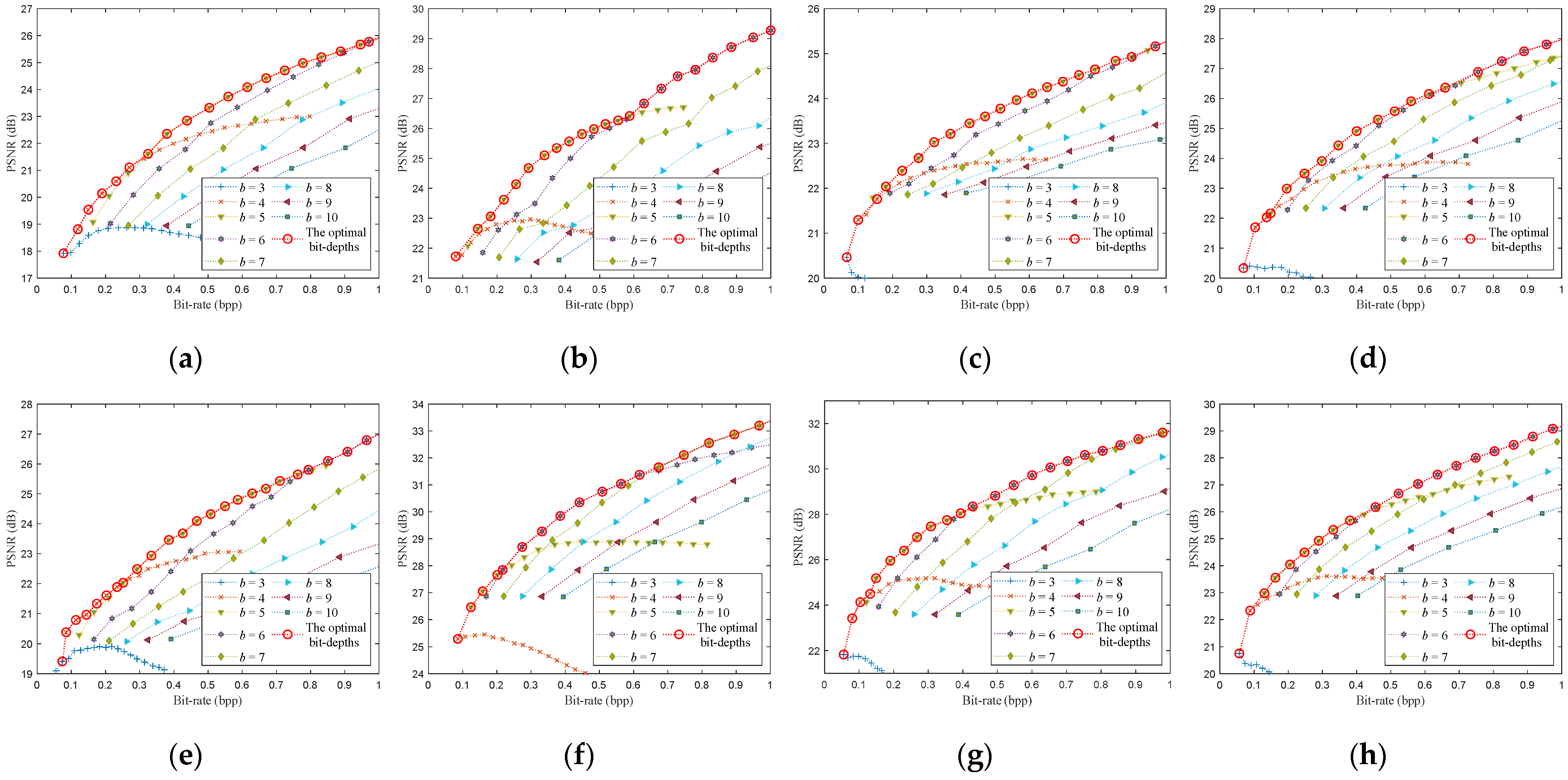
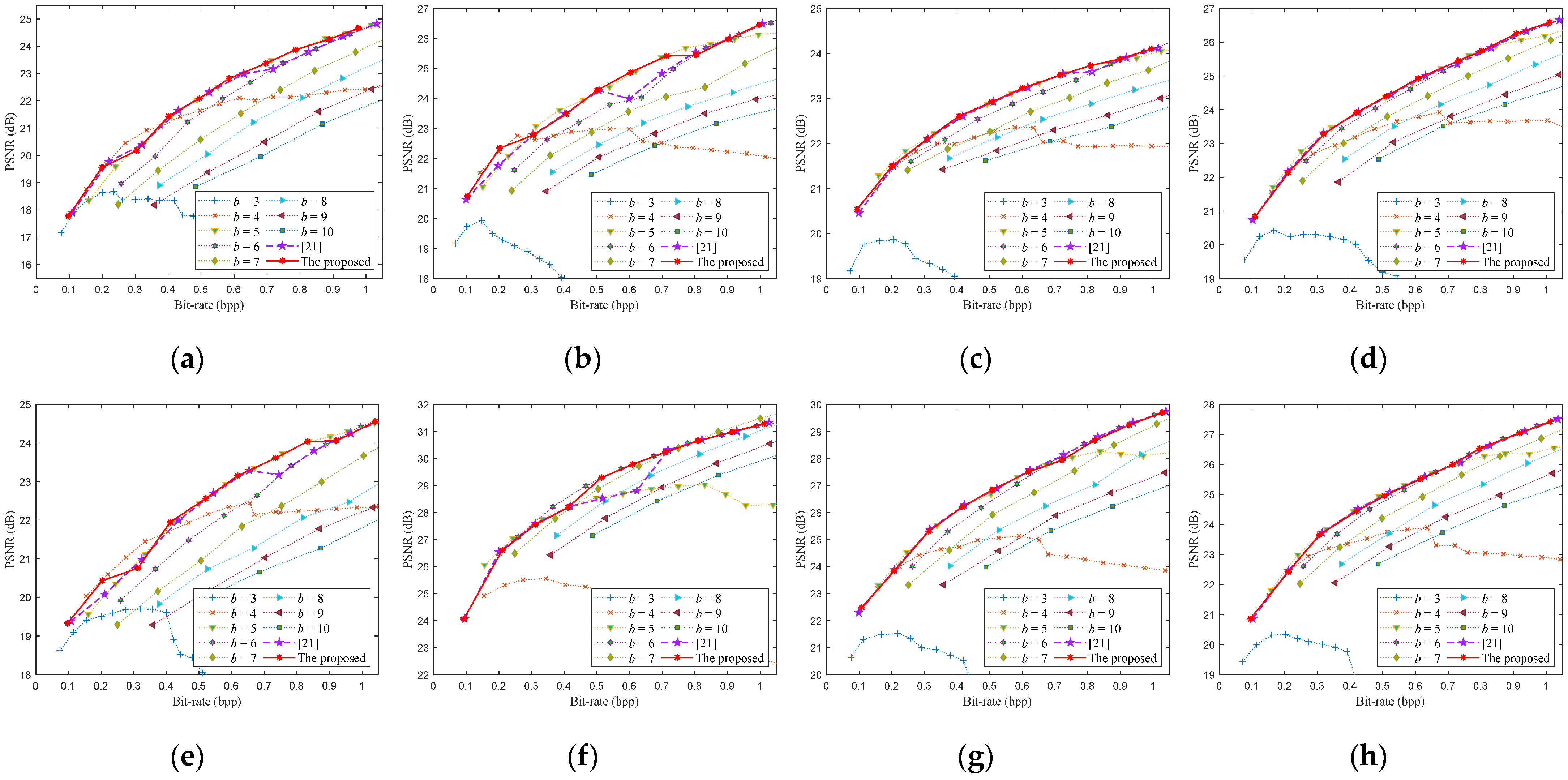
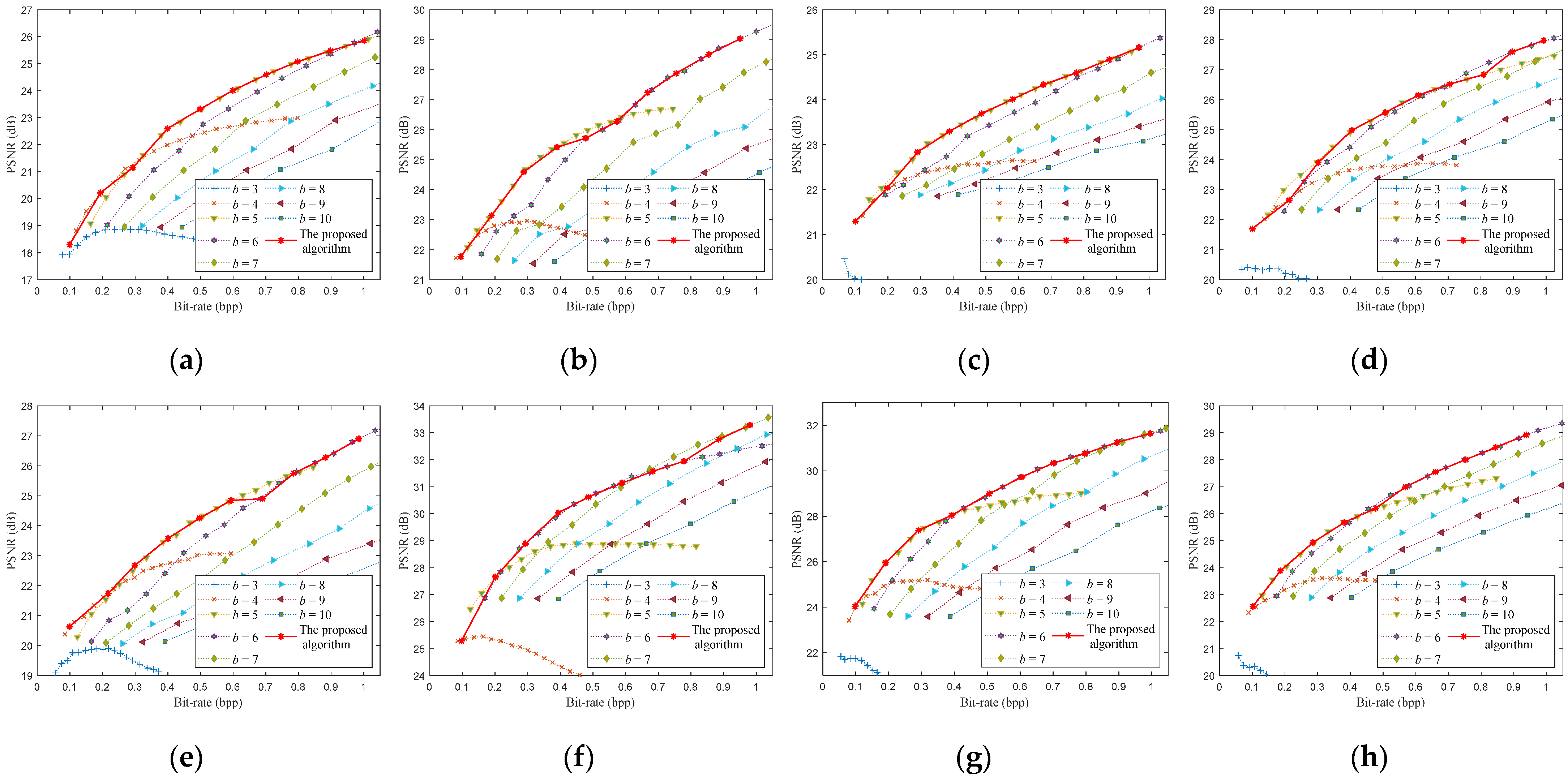
6.2. Rate-Distortion Optimization Performance
7. Conclusions
Author Contributions
Funding
Institutional Review Board Statement
Informed Consent Statement
Data Availability Statement
Conflicts of Interest
References
- Candès, E.J.; Romberg, J.; Tao, T. Robust Uncertainty Principles: Exact Signal Frequency Information. IEEE Trans. Inf. Theory 2006, 52, 489–509. [Google Scholar] [CrossRef] [Green Version]
- Donoho, D.L. Compressed sensing. IEEE Trans. Inf. Theory 2006, 52, 1289–1306. [Google Scholar] [CrossRef]
- Baraniuk, R.G. Compressive sensing. IEEE Signal Process. Mag. 2007, 24, 118–121. [Google Scholar] [CrossRef]
- Wakin, M.B.; Laska, J.N.; Duarte, M.F.; Baron, D.; Sarvotham, S.; Takhar, D.; Kelly, K.F.; Baraniuk, R.G. An architecture for compressive imaging. In Proceedings of the International Conference on Image Processing, Atlanta, GA, USA, 8–11 October 2006. [Google Scholar]
- Romberg, J. Imaging via compressive sampling. IEEE Signal Process. Mag. 2008, 25, 14–20. [Google Scholar] [CrossRef]
- Goyal, V.K.; Fletcher, A.K.; Rangan, S. Compressive sampling and lossy compression: Do random measurements provide an efficient method of representing sparse signals? IEEE Signal Process. Mag. 2008, 25, 48–56. [Google Scholar] [CrossRef]
- Li, X.; Lan, X.; Yang, M.; Xue, J.; Zheng, N. Efficient lossy compression for compressive sensing acquisition of images in compressive sensing imaging systems. Sensors 2014, 14, 23398–23418. [Google Scholar] [CrossRef] [Green Version]
- Gan, L. Block compressed sensing of natural images. In Proceedings of the 15th International Conference on Digital Signal Processing, Wales, UK, 1–4 July 2007; pp. 403–406. [Google Scholar]
- Unde, A.S.; Deepthi, P.P. Block compressive sensing: Individual and joint reconstruction of correlated images. J. Vis. Commun. Image Represent. 2017, 44, 187–197. [Google Scholar] [CrossRef]
- Unde, A.S.; Deepthi, P.P. Rate–distortion analysis of structured sensing matrices for block compressive sensing of images. Signal Process. Image Commun. 2018, 65, 115–127. [Google Scholar] [CrossRef]
- Fletcher, A.K.; Rangan, S.; Goyal, V.K. On the rate-distortion performance of compressed sensing. In Proceedings of the IEEE International Conference on Acoustics, Speech and Signal Processing, Honolulu, HI, USA, 15–20 April 2007; Volume 3, pp. 885–888. [Google Scholar]
- Mun, S.; Fowler, J.E. DPCM for quantized block-based compressed sensing of images. In Proceedings of the 20th European Signal Processing Conference, Bucharest, Romania, 27–31 August 2012; pp. 1424–1428. [Google Scholar]
- Wang, L.; Wu, X.; Shi, G. Binned progressive quantization for compressive sensing. IEEE Trans. Image Process. 2012, 21, 2980–2990. [Google Scholar] [CrossRef]
- Chen, Z.; Hou, X.; Qian, X.; Gong, C. Efficient and Robust Image Coding and Transmission Based on Scrambled Block Compressive Sensing. IEEE Trans. Multimed. 2018, 20, 1610–1621. [Google Scholar] [CrossRef]
- Chen, Z.; Hou, X.; Shao, L.; Gong, C.; Qian, X.; Huang, Y.; Wang, S. Compressive Sensing Multi-Layer Residual Coefficients for Image Coding. IEEE Trans. Circuits Syst. Video Technol. 2020, 30, 1109–1120. [Google Scholar] [CrossRef]
- Li, X.; Lan, X.; Yang, M.; Xue, J.; Zheng, N. Universal and low-complexity quantizer design for compressive sensing image coding. In Proceedings of the 2013 Visual Communications and Image Processing, Kuching, Malaysia, 17–20 November 2013; pp. 1–5. [Google Scholar]
- Zhang, J.; Zhao, D.; Jiang, F. Spatially directional predictive coding for block-based compressive sensing of natural images. In Proceedings of the 2013 IEEE International Conference on Image Processing, Melbourne, Australia, 15–18 September 2013; pp. 1021–1025. [Google Scholar]
- Shirazinia, A.; Chatterjee, S.; Skoglund, M. Analysis-by-synthesis quantization for compressed sensing measurements. IEEE Trans. Signal Process. 2013, 61, 5789–5800. [Google Scholar] [CrossRef] [Green Version]
- Gu, X.; Tu, S.; Shi, H.J.M.; Case, M.; Needell, D.; Plan, Y. Optimizing Quantization for Lasso Recovery. IEEE Signal Process. Lett. 2018, 25, 45–49. [Google Scholar] [CrossRef]
- Laska, J.N.; Baraniuk, R.G. Regime change: Bit-depth versus measurement-rate in compressive sensing. IEEE Trans. Signal Process. 2012, 60, 3496–3505. [Google Scholar] [CrossRef]
- Chen, Q.; Chen, D.; Gong, J.; Ruan, J. Low-complexity rate-distortion optimization of sampling rate and bit-depth for compressed sensing of images. Entropy 2020, 22, 125. [Google Scholar] [CrossRef] [PubMed] [Green Version]
- Jiang, W.; Yang, J. The Rate-Distortion Optimized Compressive Sensing for Image Coding. J. Signal Process. Syst. 2017, 86, 85–97. [Google Scholar] [CrossRef]
- Liu, H.; Song, B.; Tian, F.; Qin, H. Joint sampling rate and bit-depth optimization in compressive video sampling. IEEE Trans. Multimed. 2014, 16, 1549–1562. [Google Scholar] [CrossRef]
- Huang, J.; Mumford, D. Statistics of natural images and models. In Proceedings of the 1999 IEEE Computer Society Conference on Computer Vision and Pattern Recognition, Fort Collins, CO, USA, 23–25 June 1999; Volume 1. [Google Scholar]
- Lam, E.Y.; Goodman, J.W. A mathematical analysis of the DCT coefficient distributions for images. IEEE Trans. Image Process. 2000, 9, 1661–1666. [Google Scholar] [CrossRef] [PubMed] [Green Version]
- Pudi, V.; Chattopadhyay, A.; Lam, K.Y. Efficient and Lightweight Quantized Compressive Sensing using μ-Law. In Proceedings of the IEEE International Symposium on Circuits and Systems, Florence, Italy, 27–30 May 2018. [Google Scholar]
- Wang, Z.; Bovik, A.C.; Sheikh, H.R.; Simoncelli, E.P. Image quality assessment: From error visibility to structural similarity. IEEE Trans. Image Process. 2004, 13, 600–612. [Google Scholar] [CrossRef] [Green Version]
- Jordi Ribas-Corbera, S.L. Rate Control in DCT Video Coding for Low-Delay Communications. IEEE Trans. Circuits Syst. Video Technol. 1997, 9, 172–185. [Google Scholar] [CrossRef]
- Wu, X. Lossless compression of continuous-tone images via context selection, quantization, and modeling. IEEE Trans. Image Process. 1997, 6, 656–664. [Google Scholar]
- Qian, C.; Zheng, B.; Lin, B. Nonuniform quantization for block-based compressed sensing of images in differential pulse-code modulation framework. In Proceedings of the 2014 2nd International Conference on Systems and Informatics, Shanghai, China, 15–17 November 2015; pp. 791–795. [Google Scholar]
- Aiazzi, B.; Alparone, L.; Baronti, S. Estimation based on entropy matching for generalized Gaussian PDF modeling. IEEE Signal Process. Lett. 1999, 6, 138–140. [Google Scholar] [CrossRef]
- Kennedy, J.; Eberhart, R. Particle swarm optimization. In Proceedings of the IEEE International Conference on Neural Networks, Perth, Australia, 27 November–1 December 1995; Volume 4, pp. 1942–1948. [Google Scholar]
- Wang, D.; Tan, D.; Liu, L. Particle swarm optimization algorithm: An overview. Soft Comput. 2018, 22, 387–408. [Google Scholar] [CrossRef]
- Svozil, D.; Kvasnicka, V.; Pospichal, J. Introduction to multi-layer feed-forward neural networks. Chemom. Intell. Lab. Syst. 1997, 39, 43–62. [Google Scholar] [CrossRef]
- Tamura, S.; Tateishi, M. Capabilities of a four-layered feedforward neural network: Four layers versus three. IEEE Trans. Neural Networks 1997, 8, 251–255. [Google Scholar] [CrossRef] [PubMed]
- Sadeghi, B.H.M. BP-neural network predictor model for plastic injection molding process. J. Mater. Process. Technol. 2000, 103, 411–416. [Google Scholar] [CrossRef]
- Ayoobkhan, M.U.A.; Chikkannan, E.; Ramakrishnan, K. Lossy image compression based on prediction error and vector quantisation. Eurasip J. Image Video Process. 2017, 2017, 35. [Google Scholar] [CrossRef] [Green Version]
- Arbeláez, P.; Maire, M.; Fowlkes, C.; Malik, J. Contour detection and hierarchical image segmentation. IEEE Trans. Pattern Anal. Mach. Intell. 2011, 33, 898–916. [Google Scholar] [CrossRef] [Green Version]
- Roth, S.; Black, M.J. Fields of experts. Int. J. Comput. Vis. 2009, 82, 205–229. [Google Scholar] [CrossRef]
- Skretting, K. Huffman Coding and Arithmetic Coding. Available online: https://www.mathworks.com/matlabcentral/fileexchange/2818-huffman-coding-and-arithmetic-coding (accessed on 13 October 2020).
- Mun, S.; Fowler, J.E. Block compressed sensing of images using directional transforms. In Proceedings of the 16th IEEE International Conference on Image Processing, Cairo, Egypt, 7–10 November 2009; pp. 3021–3024. [Google Scholar]
- Lee Rodgers, J.; Alan Nice Wander, W. Thirteen ways to look at the correlation coefficient. Am. Stat. 1988, 42, 59–66. [Google Scholar] [CrossRef]


| Quantization Framework | PCC | MSE | ||||||
|---|---|---|---|---|---|---|---|---|
| DPCM-plus-SQ | −3.0927 × 10⁻¹ | 1.9128 × 10⁻² | −1.6845 × 10⁻¹ | 1.6592 × 10⁻¹ | 1.3467 | −1.1718 | 0.995 | 0.022 |
| uniform SQ | −2.0660 × 10⁻¹ | 6.5594 × 10⁻³ | −2.0673 × 10⁻¹ | 2.3831 × 10⁻¹ | 1.2761 | −1.9910 | 0.996 | 0.027 |
| Quantization Framework | DPCM-Plus-SQ | Uniform SQ | ||
|---|---|---|---|---|
| Data | Training Set | Test Set | Training Set | Test Set |
| Accuracy (%) | 80.7 | 70.7 | 76.5 | 70.4 |
| Percentage of one-bit error (%) | 19.3 | 29.0 | 23.5 | 29.3 |
| Sum (above) (%) | 100 | 99.7 | 100 | 99.7 |
| Image | Target Bit-Rate (bpp) | 0.1 | 0.2 | 0.3 | 0.4 | 0.5 | |
| BSD68 test set | Actual bit-rate | Maximum | 0.110 | 0.218 | 0.327 | 0.427 | 0.523 |
| Minimum | 0.087 | 0.181 | 0.268 | 0.368 | 0.467 | ||
| Average | 0.099 | 0.203 | 0.305 | 0.406 | 0.503 | ||
| Average of absolute error percentage (%) | 3.23 | 2.91 | 2.29 | 2.33 | 1.78 | ||
| Image | Target Bit-Rate (bpp) | 0.6 | 0.7 | 0.8 | 0.9 | 1 | |
| BSD68 test set | Actual bit-rate | Maximum | 0.619 | 0.727 | 0.831 | 0.934 | 1.037 |
| Minimum | 0.565 | 0.664 | 0.771 | 0.831 | 0.916 | ||
| Average | 0.603 | 0.706 | 0.805 | 0.901 | 0.999 | ||
| Average of absolute error percentage (%) | 1.67 | 1.87 | 1.65 | 1.86 | 1.86 | ||
| Image | Target Bit-Rate (bpp) | 0.1 | 0.2 | 0.3 | 0.4 | 0.5 | |
| BSD68 test set | Actual bit-rate | Maximum | 0.108 | 0.219 | 0.319 | 0.424 | 0.533 |
| Minimum | 0.090 | 0.187 | 0.274 | 0.366 | 0.457 | ||
| Average | 0.101 | 0.200 | 0.299 | 0.399 | 0.499 | ||
| Average of absolute error percentage (%) | 3.17 | 2.75 | 2.30 | 2.09 | 2.03 | ||
| Image | Target Bit-Rate (bpp) | 0.6 | 0.7 | 0.8 | 0.9 | 1 | |
| BSD68 test set | Actual bit-rate | Maximum | 0.636 | 0.741 | 0.848 | 0.954 | 1.063 |
| Minimum | 0.548 | 0.646 | 0.737 | 0.829 | 0.922 | ||
| Average | 0.597 | 0.695 | 0.793 | 0.891 | 0.989 | ||
| Average of absolute error percentage (%) | 2.18 | 2.23 | 2.20 | 2.33 | 2.26 | ||
| Target Bit-Rate (bpp) | Actual Bit-Rate (bpp) | |||||||
|---|---|---|---|---|---|---|---|---|
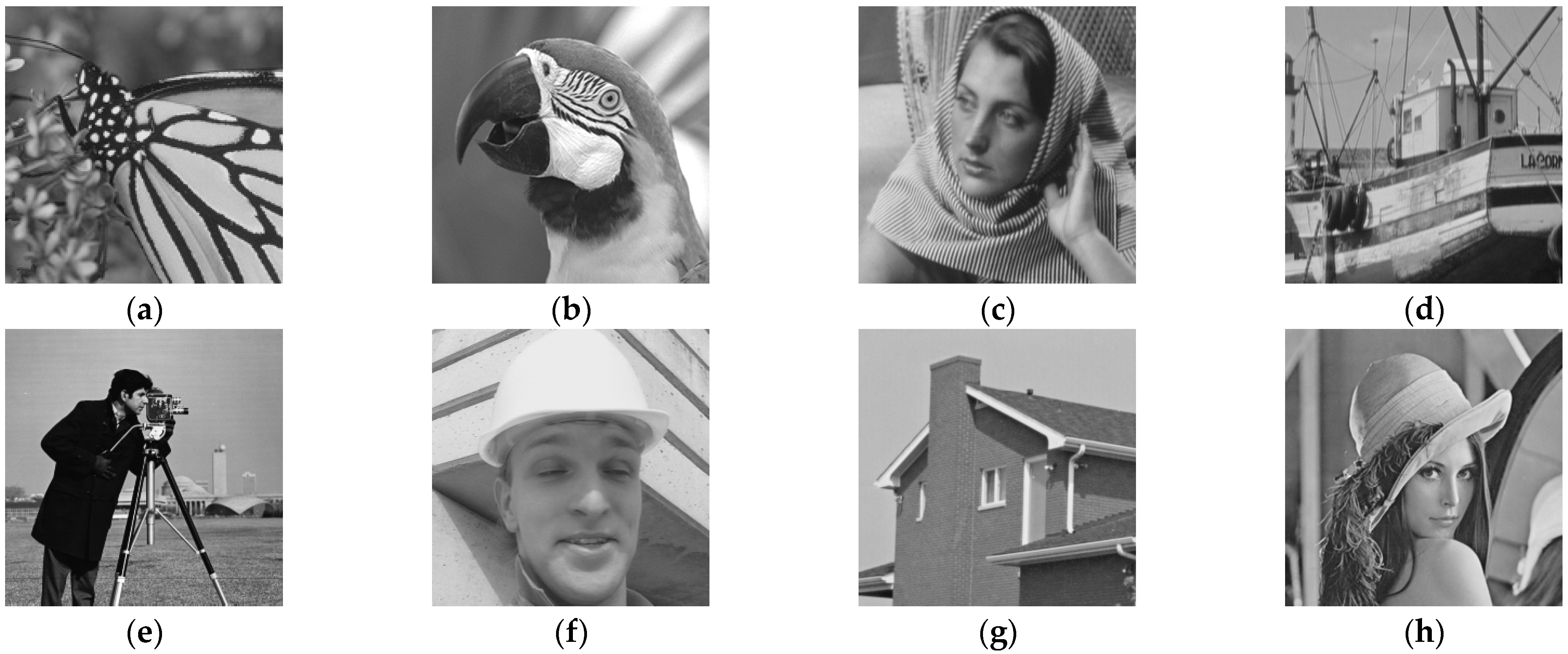
| Monarch | Parrots | Barbara | Boats | Cameraman | Foreman | House | Lena | |
| 0.1 | 0.102 | 0.102 | 0.098 | 0.106 | 0.101 | 0.096 | 0.105 | 0.100 |
| 0.2 | 0.203 | 0.207 | 0.204 | 0.207 | 0.204 | 0.208 | 0.204 | 0.205 |
| 0.3 | 0.305 | 0.305 | 0.307 | 0.317 | 0.312 | 0.308 | 0.310 | 0.307 |
| 0.4 | 0.408 | 0.402 | 0.412 | 0.416 | 0.419 | 0.415 | 0.414 | 0.412 |
| 0.5 | 0.493 | 0.506 | 0.504 | 0.513 | 0.518 | 0.512 | 0.511 | 0.507 |
| 0.6 | 0.590 | 0.606 | 0.606 | 0.615 | 0.623 | 0.609 | 0.612 | 0.609 |
| 0.7 | 0.694 | 0.713 | 0.713 | 0.725 | 0.731 | 0.712 | 0.720 | 0.705 |
| 0.8 | 0.790 | 0.800 | 0.802 | 0.827 | 0.837 | 0.812 | 0.817 | 0.805 |
| 0.9 | 0.884 | 0.905 | 0.905 | 0.918 | 0.897 | 0.917 | 0.923 | 0.910 |
| 1.0 | 0.981 | 1.003 | 1.003 | 1.019 | 1.030 | 1.017 | 1.024 | 1.007 |
| Target Bit-Rate (bpp) | Actual Bit-Rate (bpp) | |||||||
|---|---|---|---|---|---|---|---|---|
| Monarch | Parrots | Barbara | Boats | Cameraman | Foreman | House | Lena | |
| 0.1 | 0.102 | 0.098 | 0.099 | 0.103 | 0.101 | 0.095 | 0.098 | 0.102 |
| 0.2 | 0.197 | 0.189 | 0.201 | 0.210 | 0.201 | 0.202 | 0.190 | 0.187 |
| 0.3 | 0.303 | 0.292 | 0.295 | 0.308 | 0.302 | 0.296 | 0.291 | 0.289 |
| 0.4 | 0.404 | 0.392 | 0.387 | 0.410 | 0.404 | 0.398 | 0.407 | 0.380 |
| 0.5 | 0.504 | 0.487 | 0.490 | 0.511 | 0.500 | 0.494 | 0.505 | 0.477 |
| 0.6 | 0.603 | 0.578 | 0.593 | 0.611 | 0.596 | 0.598 | 0.610 | 0.569 |
| 0.7 | 0.705 | 0.671 | 0.691 | 0.703 | 0.695 | 0.706 | 0.703 | 0.668 |
| 0.8 | 0.799 | 0.756 | 0.779 | 0.811 | 0.794 | 0.792 | 0.804 | 0.759 |
| 0.9 | 0.899 | 0.864 | 0.881 | 0.902 | 0.896 | 0.895 | 0.898 | 0.848 |
| 1.0 | 1.014 | 0.957 | 0.969 | 0.993 | 0.989 | 0.996 | 1.004 | 0.940 |
| Image | Target Bit-Rate (bpp) | 0.1 | 0.2 | 0.3 | 0.4 | 0.5 |
| BSD68 test set | Optimal percentage (%) | 91.18 | 64.71 | 77.94 | 77.94 | 64.71 |
| One-bit error percentage (%) | 8.82 | 35.29 | 22.06 | 22.06 | 35.29 | |
| Sum of the above (%) | 100 | 100 | 100 | 100 | 100 | |
| Average PSNR error (dB) | −0.04 | −0.13 | −0.12 | −0.06 | −0.08 | |
| Image | Target Bit-Rate (bpp) | 0.6 | 0.7 | 0.8 | 0.9 | 1 |
| BSD68 test set | Optimal percentage (%) | 63.24 | 54.41 | 60.29 | 57.35 | 64.71 |
| One-bit error percentage (%) | 36.76 | 45.59 | 39.71 | 41.18 | 33.82 | |
| Sum of the above (%) | 100 | 100 | 100 | 98.53 | 98.53 | |
| Average PSNR error (dB) | −0.09 | −0.10 | −0.08 | −0.11 | −0.07 |
| Image | Target Bit-Rate (bpp) | 0.1 | 0.2 | 0.3 | 0.4 | 0.5 |
| BSD68 test set | Optimal percentage (%) | 82.35 | 58.82 | 79.41 | 79.41 | 76.47 |
| One-bit error percentage (%) | 17.65 | 41.18 | 20.59 | 20.59 | 23.53 | |
| Sum of the above (%) | 100 | 100 | 100 | 100 | 100 | |
| Average PSNR error (dB) | −0.29 | −0.21 | −0.16 | −0.06 | −0.07 | |
| Image | Target Bit-Rate (bpp) | 0.6 | 0.7 | 0.8 | 0.9 | 1 |
| BSD68 test set | Optimal percentage (%) | 64.71 | 70.59 | 60.29 | 55.88 | 63.24 |
| One-bit error percentage (%) | 35.29 | 29.41 | 38.24 | 42.65 | 35.29 | |
| Sum of the above (%) | 100 | 100 | 98.53 | 98.53 | 98.53 | |
| Average PSNR error (dB) | −0.07 | −0.09 | −0.11 | −0.14 | −0.11 |
Publisher’s Note: MDPI stays neutral with regard to jurisdictional claims in published maps and institutional affiliations. |
© 2021 by the authors. Licensee MDPI, Basel, Switzerland. This article is an open access article distributed under the terms and conditions of the Creative Commons Attribution (CC BY) license (https://creativecommons.org/licenses/by/4.0/).
Share and Cite
Chen, Q.; Chen, D.; Gong, J. A General Rate-Distortion Optimization Method for Block Compressed Sensing of Images. Entropy 2021, 23, 1354. https://doi.org/10.3390/e23101354
Chen Q, Chen D, Gong J. A General Rate-Distortion Optimization Method for Block Compressed Sensing of Images. Entropy. 2021; 23(10):1354. https://doi.org/10.3390/e23101354
Chicago/Turabian StyleChen, Qunlin, Derong Chen, and Jiulu Gong. 2021. "A General Rate-Distortion Optimization Method for Block Compressed Sensing of Images" Entropy 23, no. 10: 1354. https://doi.org/10.3390/e23101354
APA StyleChen, Q., Chen, D., & Gong, J. (2021). A General Rate-Distortion Optimization Method for Block Compressed Sensing of Images. Entropy, 23(10), 1354. https://doi.org/10.3390/e23101354