
One- and Two-Phase Software Requirement Classification Using Ensemble Deep Learning


Abstract
:1. Introduction
- Summary, categorization, and comparison of published research on ML or DL use for classifying SRs. The summarized categories involve classifying SRs into main classes, classifying FRs into multi-classes, classifying NFRs into multi-classes, and complete systems that classify SRs into main classes and FRs and NFRs into multi-classes.
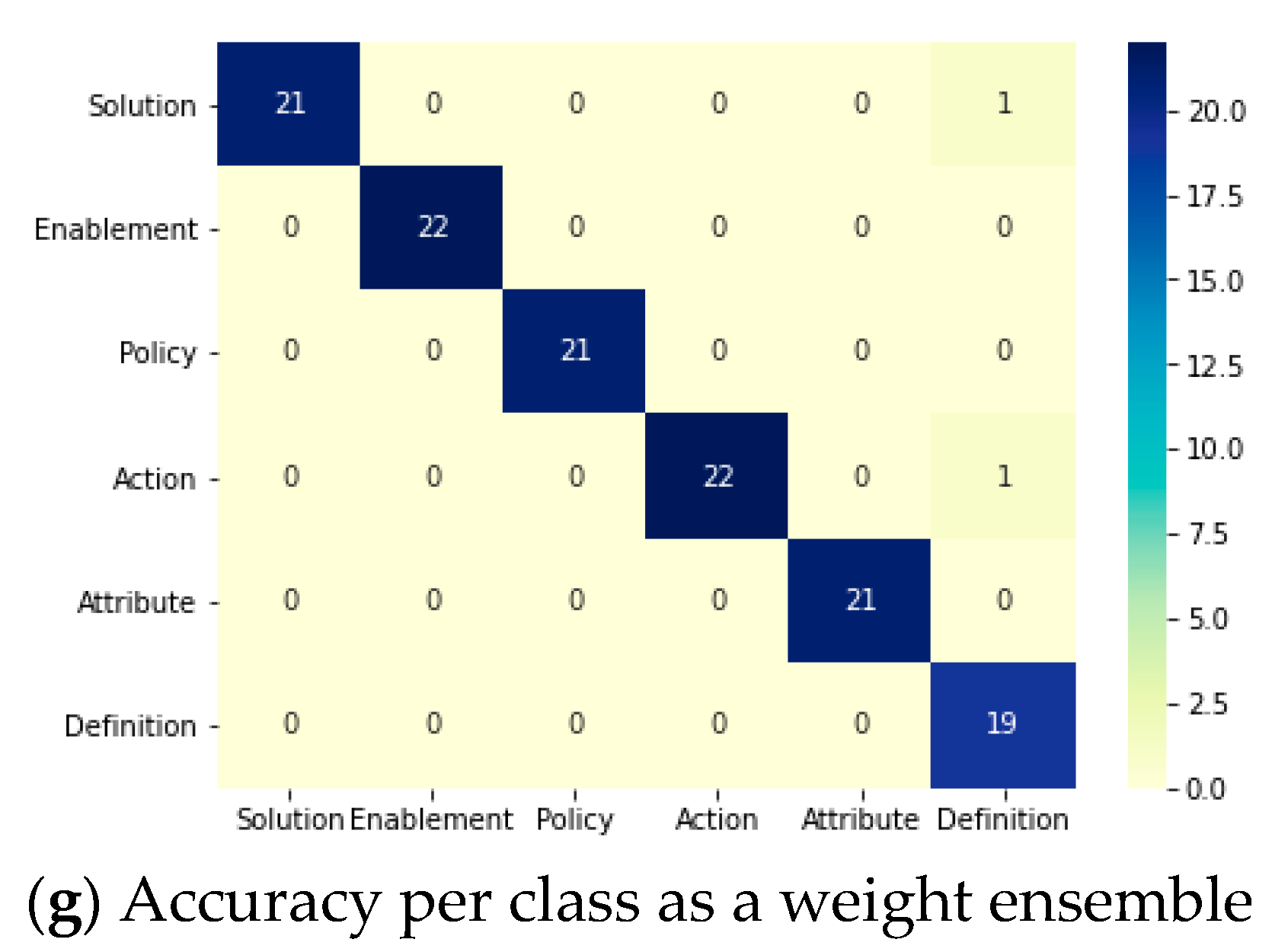
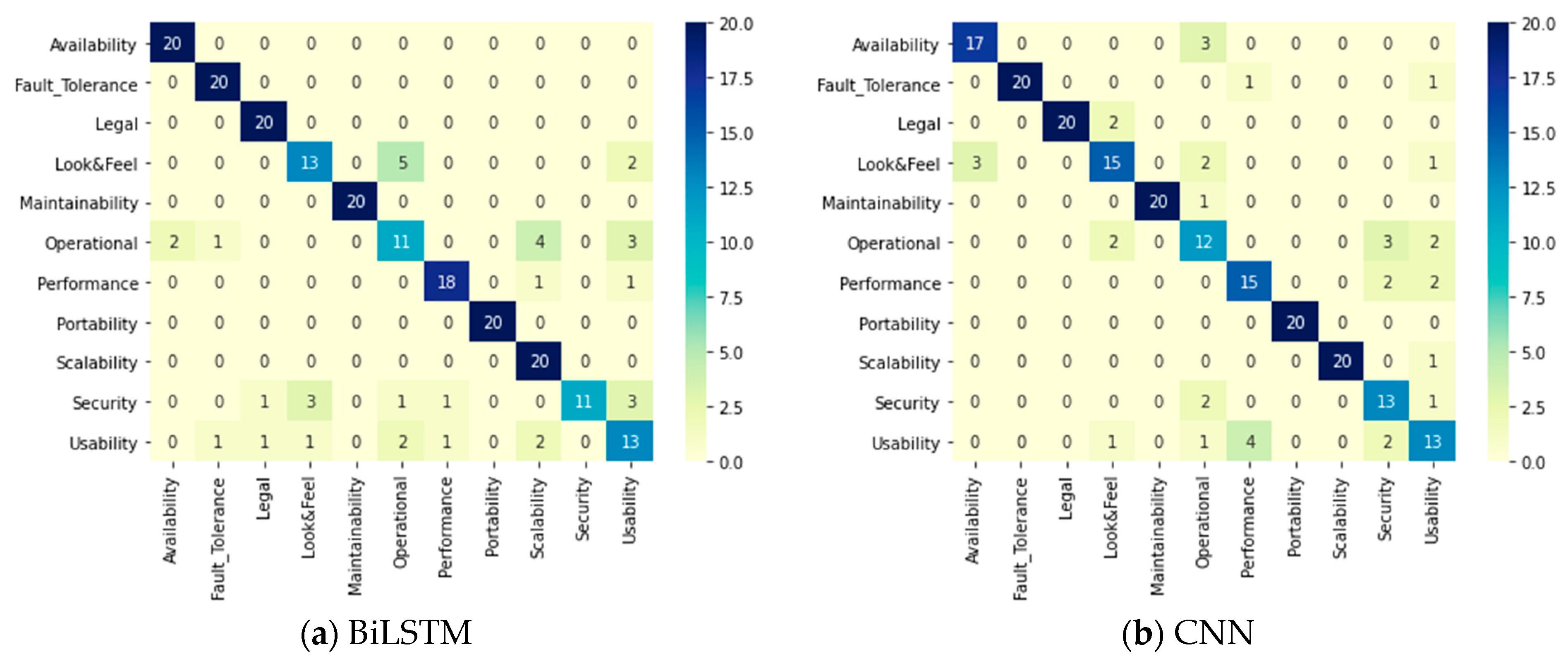
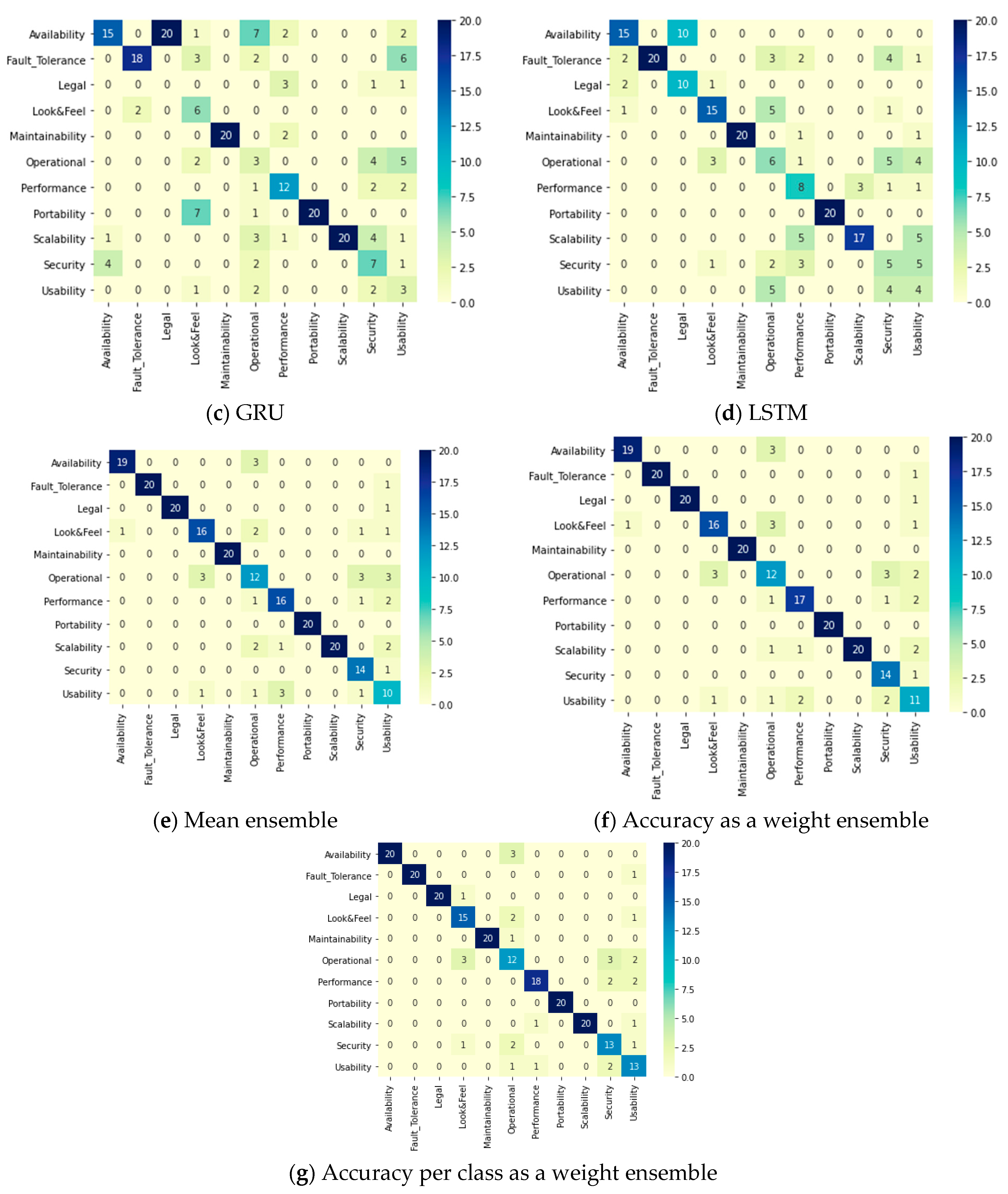
- Introduction of an ensemble learning framework based on DL models for classifying different types of SRs. The conducted experiments present comparative results between three different ensemble models—mean ensemble, accuracy as a weight ensemble, and accuracy per class as a weight ensemble—and show that accuracy per class as a weight ensemble learning classifier combining BiLSTM, LSTM, GRU, and CNN has a stronger capability to correctly predict different types of SRs.
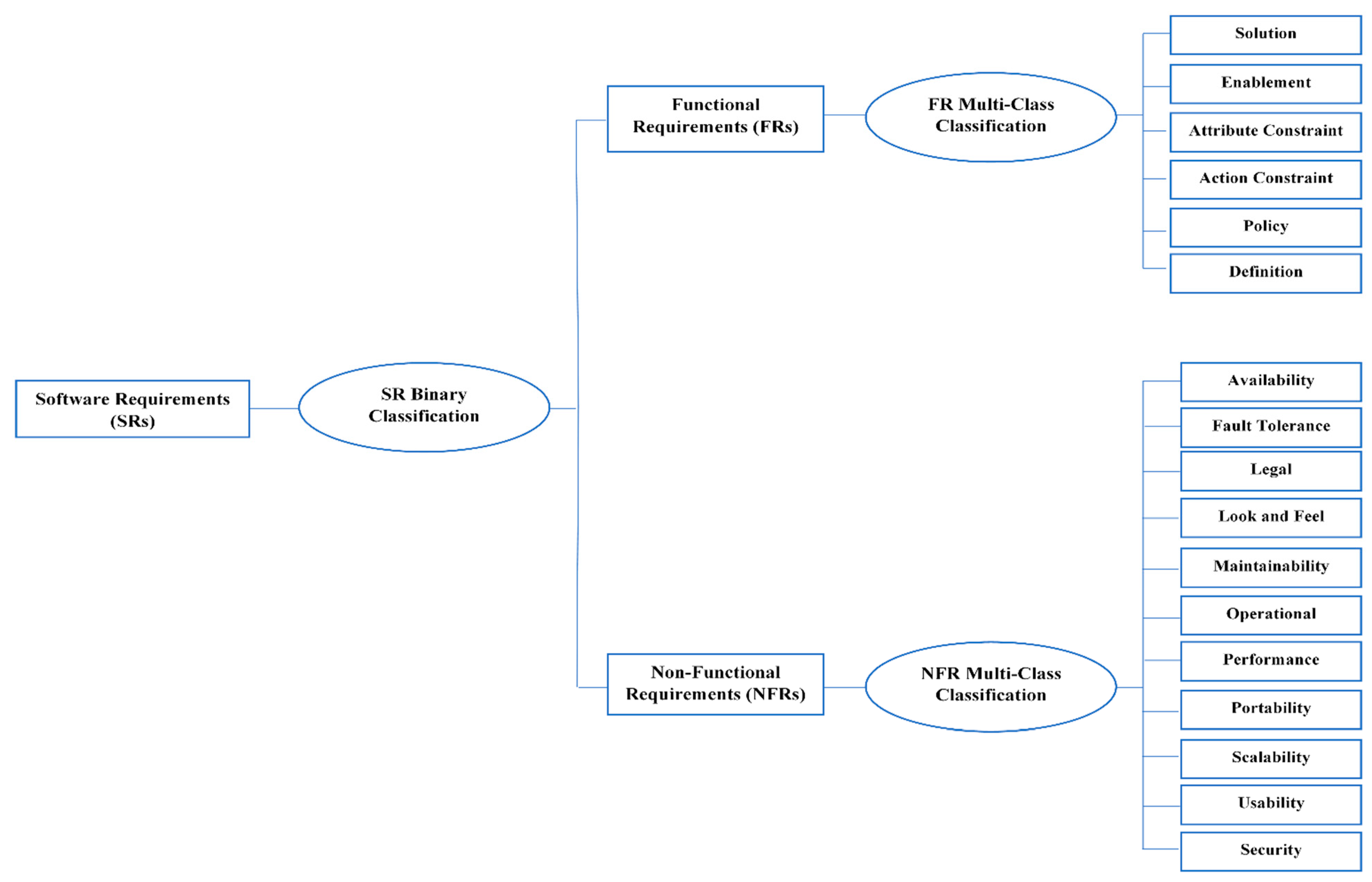
- Proposition of a two-phase system using the ensemble DL method. The first phase uses binary classification to classify SRs into FRs or NFRs, while the second phase classifies the output of the first phase (FRs or NFRs) into multi-classes. FRs are classified into six different labels: solution, enablement, action constraint, attribute constraint, policy, and definition. On the contrary, NFRs are classified into 11 different labels: availability, fault tolerance, legal and licensing, look and feel, maintainability, operability, performance, portability, scalability, security, and usability.
- Proposition of a one-phase system using the ensemble DL method. The input is SRs and the output is 17 multi-classes of either FRs or NFRs (solution, enablement, action constraint, attribute constraint, policy, definition, availability, fault tolerance, legal and licensing, look and feel, maintainability, operability, performance, portability, scalability, security, and usability).
- Investigation of the performance of each base DL classifier and a number of ensemble DL classifiers in each phase of the system.
- To the best of our knowledge there is no complete two-phase system to classify SRs into FRs or NFRs, then to classify each FR and NFR into multi-classes using ensemble DL methodology. In addition, there is no such similar categorized review summary of the previous studies on classifying SRs.
2. Related Work
2.1. Classifying SRs into Main Classes
2.2. Classifying FRs into Multi-Classes
2.3. Classifying NFRs into Multi-Classes
2.4. Complete System (Classifying NFRs and FRs into Multi-Classes)
3. Materials and Methods
3.1. Phases of Classification
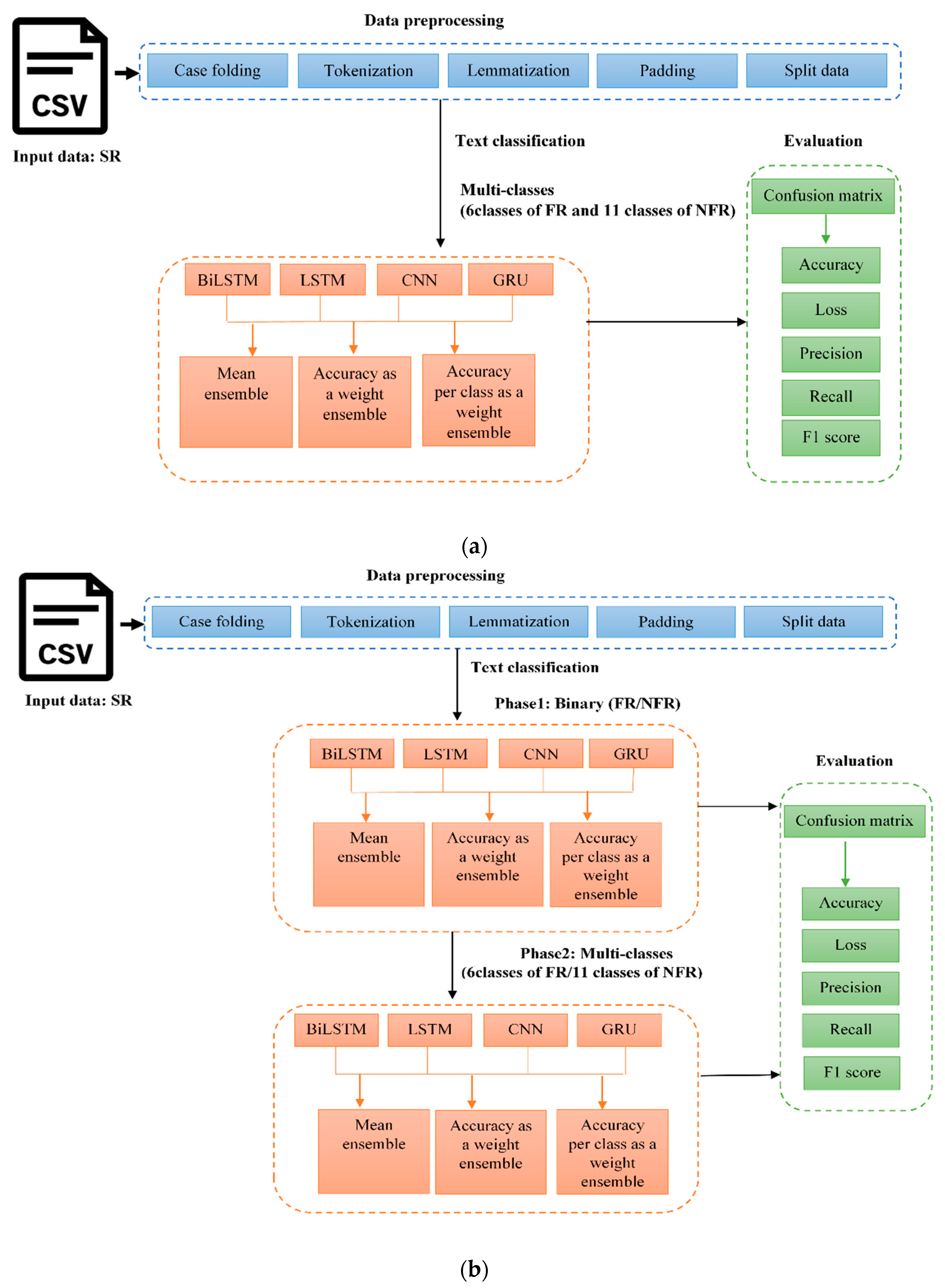
3.2. Methodology
- Data preprocessing;
- Text classification phase 1 (binary);
- Text classification phase 2 (multi-classes);
- Evaluation.
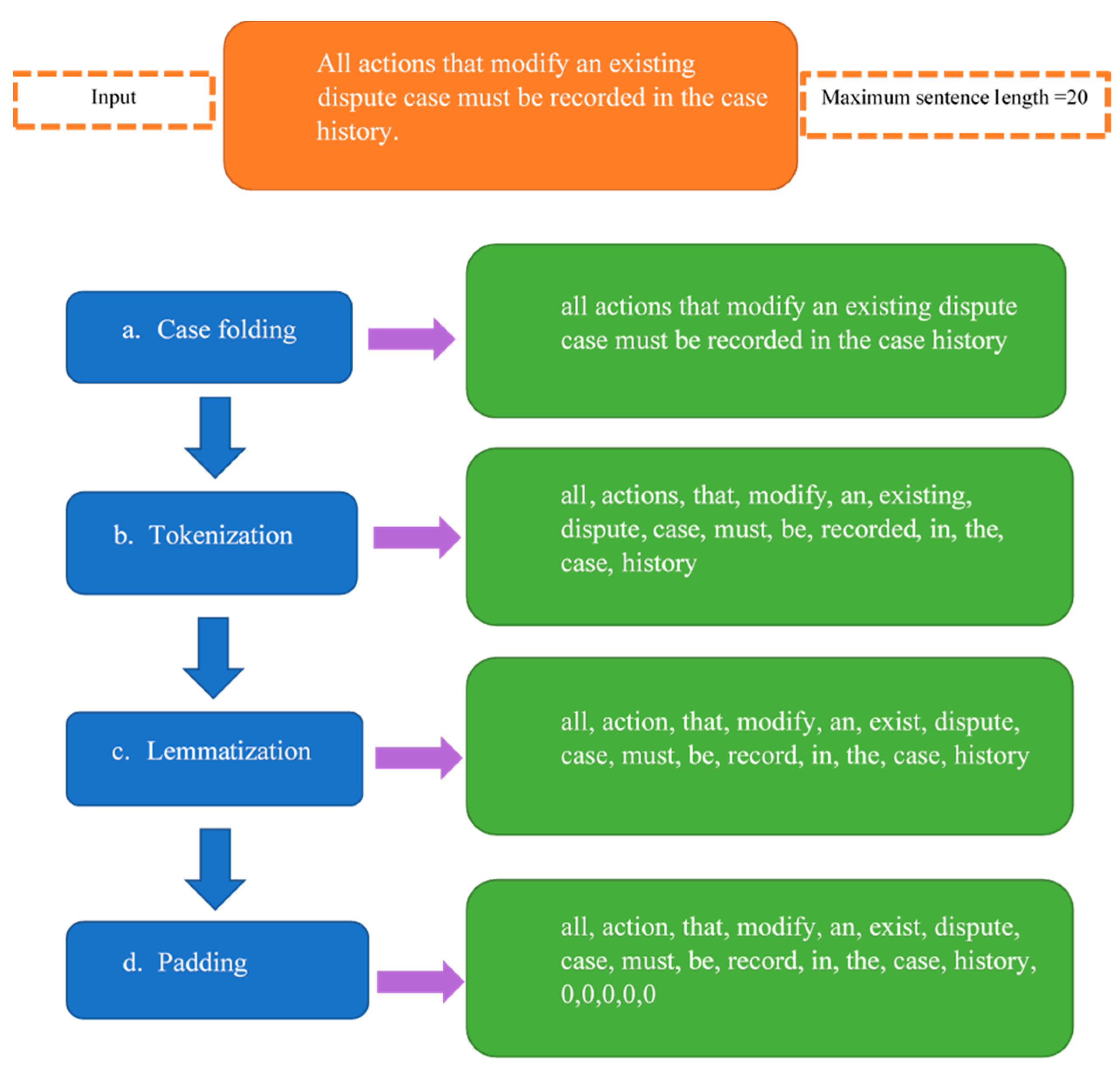
3.2.1. Data Preprocessing
| Algorithm 1 (Data preprocessing step) |
| Input: X: A data stream of sentences inserted from a file. |
| Y: a label for the inserted sentences |
| Output: |
| Train_data: a section of the X and Y to train the algorithms. |
| Validation_data: a section of the X and Y to validate the algorithms. |
| Test_data: a section of the X and Y to test the algorithms. |
| X < Tokenize sentences in X |
| X < Remove spaces and stop words. |
| X < Convector(X) // convert sentences into numbers |
| Y < Convector (Y) // convert labels (classes) into numbers |
| // split data into training, validation and testing portions |
| train_data (x, y), validation data(x,y), test_data(x,y) < Split (X, Y) |
3.2.2. Text Classification
- A.
- Base DL Classifiers:
- LSTM is a type of recurrent neural network (RNN) that uses memory blocks to solve the vanishing gradient problem in RNN using memory blocks. The model’s first layer is the input layer, which receives preprocessed data in a time step. Each component is passed to the embedding layer at first, which is represented to generate feature vectors. Then, the LSTM hidden layer follows the forward path only. LSTM has three main gates, namely, input, forget, and output gates, to control the cell state and update the weights [22].
- BiLSTM includes two hidden layers connected with both the input and the output. BiLSTM includes a forward LSTM layer and a backward LSTM layer to utilize the next tokens for learning information, and better predictions can be achieved. The best way to benefit from the BiLSTM is to stack LSTM layers. Forward layers are iterated from t = 1 to T. On the contrary, backward layers are iterated from t = T to 1 [23].
- CNNs involve producing local features by applying the convolutional concept [24]. Using filters with a width determined by the word embedding vector size, different vertical local regions allow different filter sizes of L = 2, 3, and 4. This is helpful for learning many features. Active convoluted results are used to generate feature maps with varied dimensions on the filters [25].
- GRU is type of RNN known for its fast conversions compared to LSTM. In addition, it requires fewer parameters [26]. It has two types of gates: An update gate and a reset gate. Since it has no memory to store information, it only deals with unit information. The update gate decides the amount of data to be updated and the reset gate decides the amount of past data to forget. If the gate is set to zero, it reads input data and ignores the previously calculated state [27].
- B.
- Ensemble Models:
- B.1.
- Mean Ensemble:
| Algorithm 2 (Mean ensemble for base DL classifiers) |
| Input: X: Preprocessed data. |
| Y: labels of the sentences. |
| NNAL(i): Number of Neural Network algorithms used [BiLSTM, CNN, GRU, LSTM]. |
| Output: |
| Mean_ Accuracy: Represents the Mean ensemble model. |
| For each model in NNAL(i): |
| NNL(i) < fit (train_data (X, Y), validation(X,Y)) |
| P(y′) < Predict (test data(X)) |
| Result< Compare (p(y′), Y) |
| Conf(i)< Calculate (Confusion matrix) |
| Accuracy(i) < Result/Y*100 |
| End |
| //Final prediction |
| Mean_Accuracy < mean(P(y′))/4 |
- B.2.
- Accuracy as a weight:
| Algorithm 3 Accuracy as a weight ensemble for base DL classifiers |
| Input: X: Preprocessed data. |
| Y: labels of the sentences. |
| NNAL(i): Number of Neural Network algorithms used [BiLSTM, CNN, GRU, LSTM]. |
| Output: |
| W: Weight for each NNAL which is its accuracy. |
| Voting_ Accuracy: Represents the weight as accuracy ensemble voting model. |
| For each model in NNAL(i): |
| NNL(i) < fit (train_data (X, Y), validation(X,Y)) |
| P(y′) < Predict (test data(X)) |
| Result< Compare(p(y′), Y) |
| Conf(i)< Calculate (Confusion matrix) |
| Accuracy(i) < Result/Y*100 |
| W(i) < Accuracy(i) |
| End |
| // Find the final prediction |
| V_result< Voting_algorithm (NNAL(i), W(i)) |
| Voting_ Accuracy < V_Result/Y*100 |
- B.3.
- Accuracy per class as a weight:
| Algorithm 4 Accuracy per class as a weight ensemble |
| Input: X: Preprocessed data. |
| Y: labels of the sentences |
| NNAL(i): Number of Neural Network algorithms used [BiLSTM, CNN, GRU, LSTM]. |
| Output: |
| W: An array of weights assigned for each NNAL(i) |
| Voting_ Accuracy: Represents the proposed ensemble voting model. |
| For each model in NNAL(i): |
| NNL(i) < fit (train_data (X, Y), validation_data (X, Y)) |
| P(y′) < Predict (test data(X)) |
| Result < Compare(p(y′), Y) |
| Conf(i) < Calculate (Confusion matrix) |
| Accuracy(i) < Result/Y*100 |
| End |
| // Give a weight for each model |
| // combine the diagonals of all confusion matrices into one matrix |
| Conf_matrix < [[Conf (i. diagonal]] |
| // find the maximum of each column that will represent the algorithm weight |
| W < max_coloumn (Conf_matrix(i)) |
| V_result< Voting_algorithm (NNAL(i), W(i)) |
| Voting_ Accuracy < V_Result/Y*100 |
3.2.3. Evaluation Methods
- A.
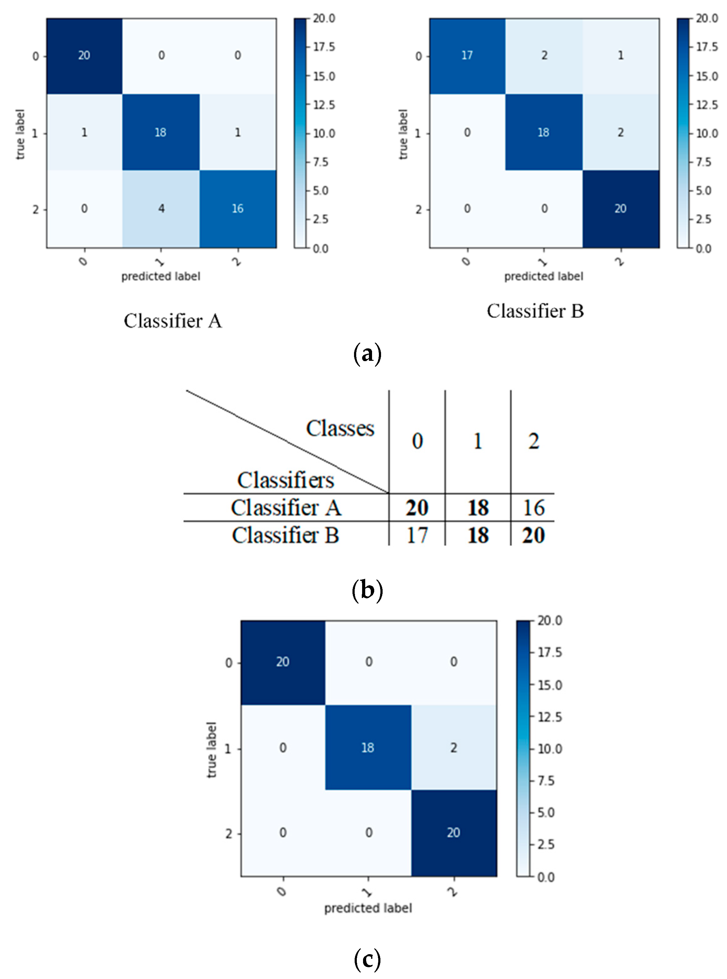
- Confusion Matrix
- B.
- Accuracy
- C.
- Loss
- D.
- Precision
- E.
- Recall
- F.
- F1 Score
4. Experiment Details
4.1. Hardware and Software Details
4.2. PROMISE Dataset
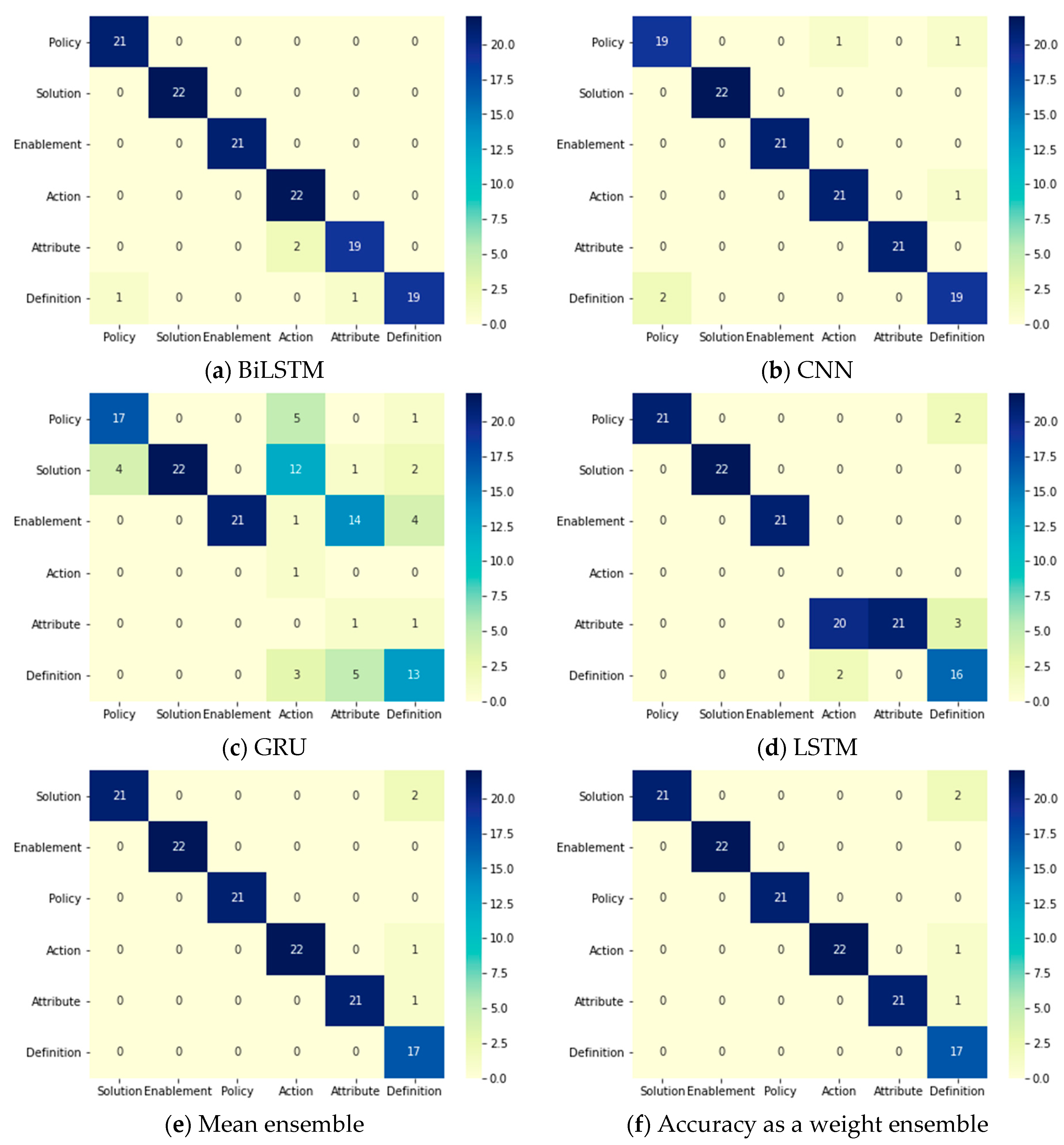
4.3. One-Phase Classification System
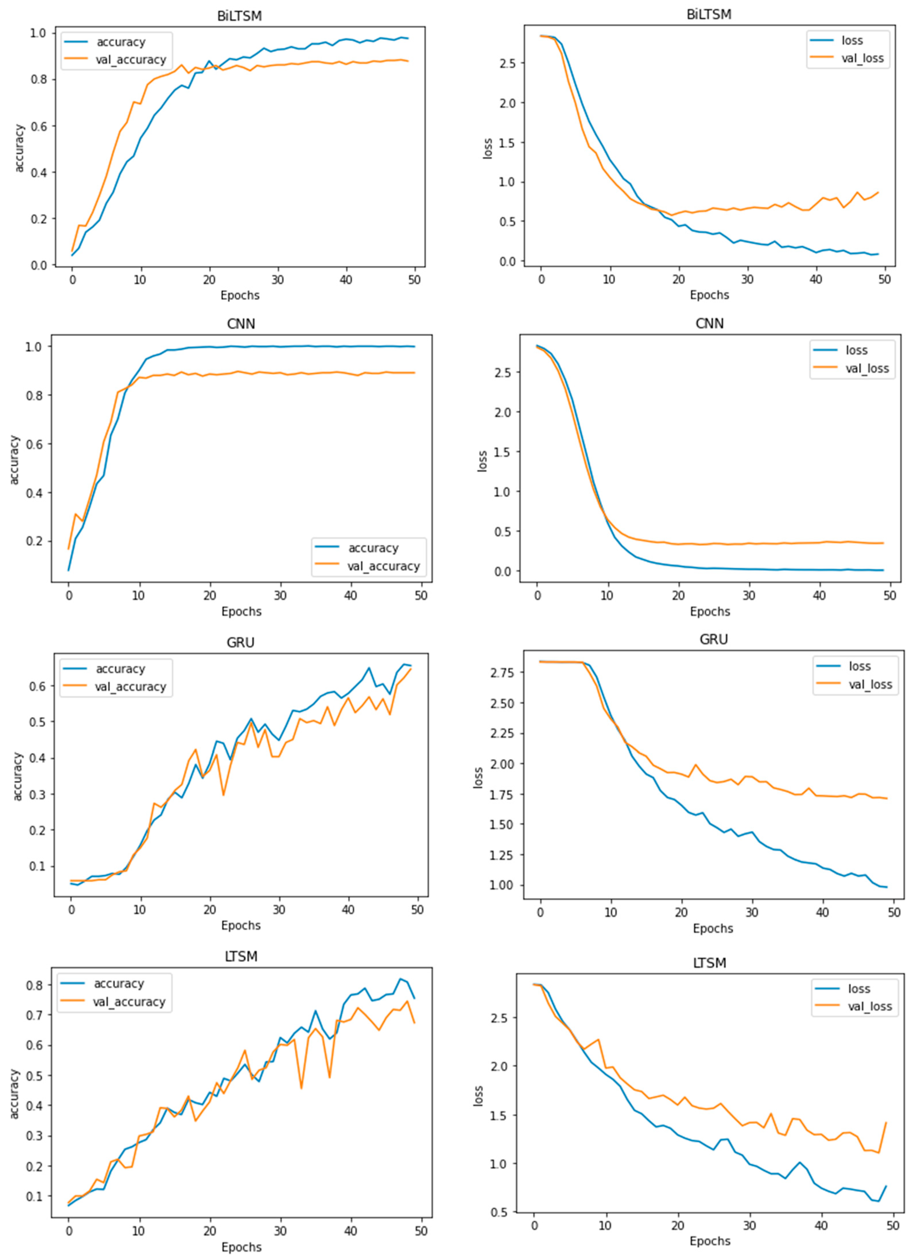
- A.
- Training
- B.
- Test Results and Discussion
4.4. Two-Phase Classification System
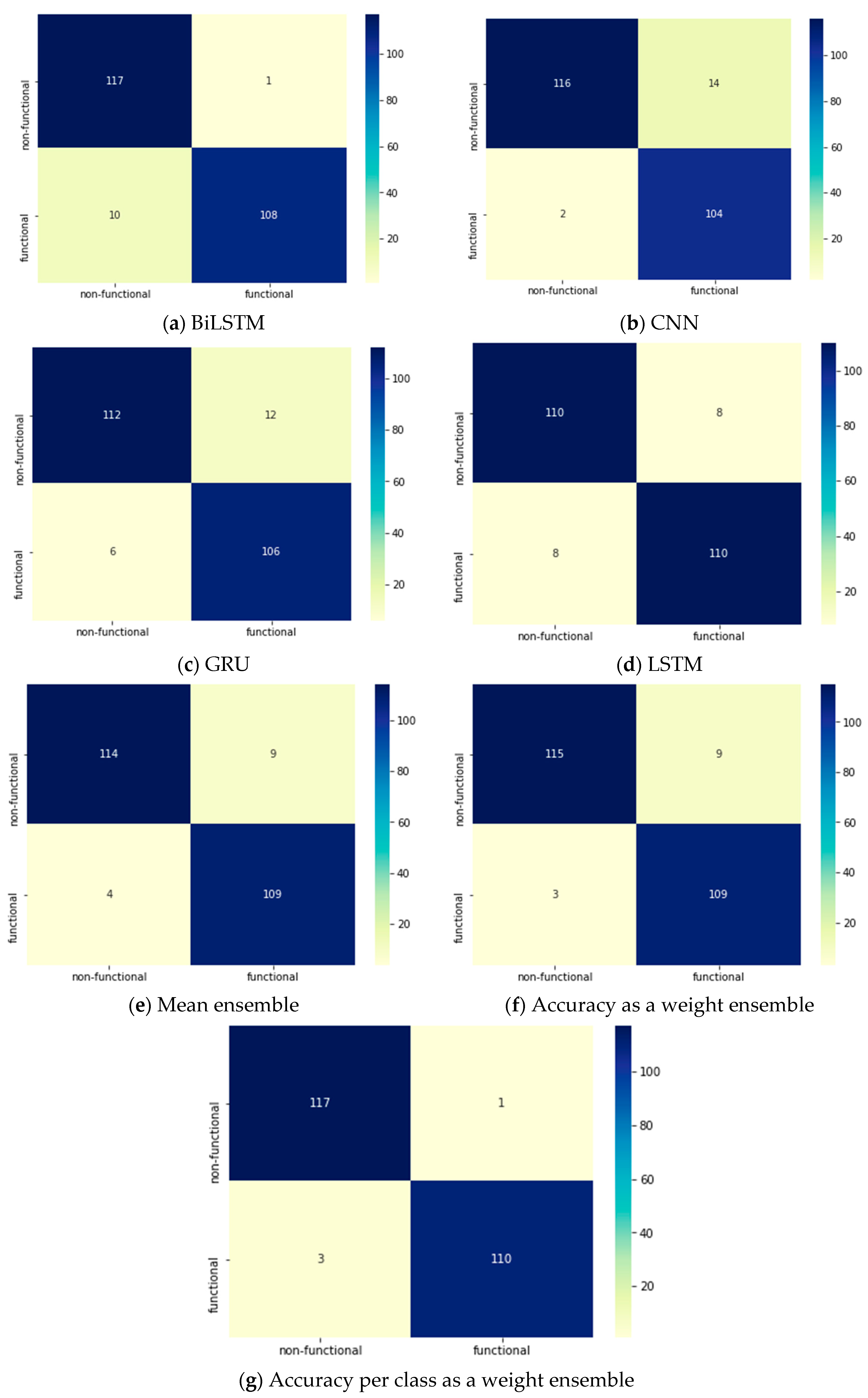
4.4.1. Binary Classification of SRs into an FR or NFR Phase
- A.
- Training
- B.
- Test Results and discussion
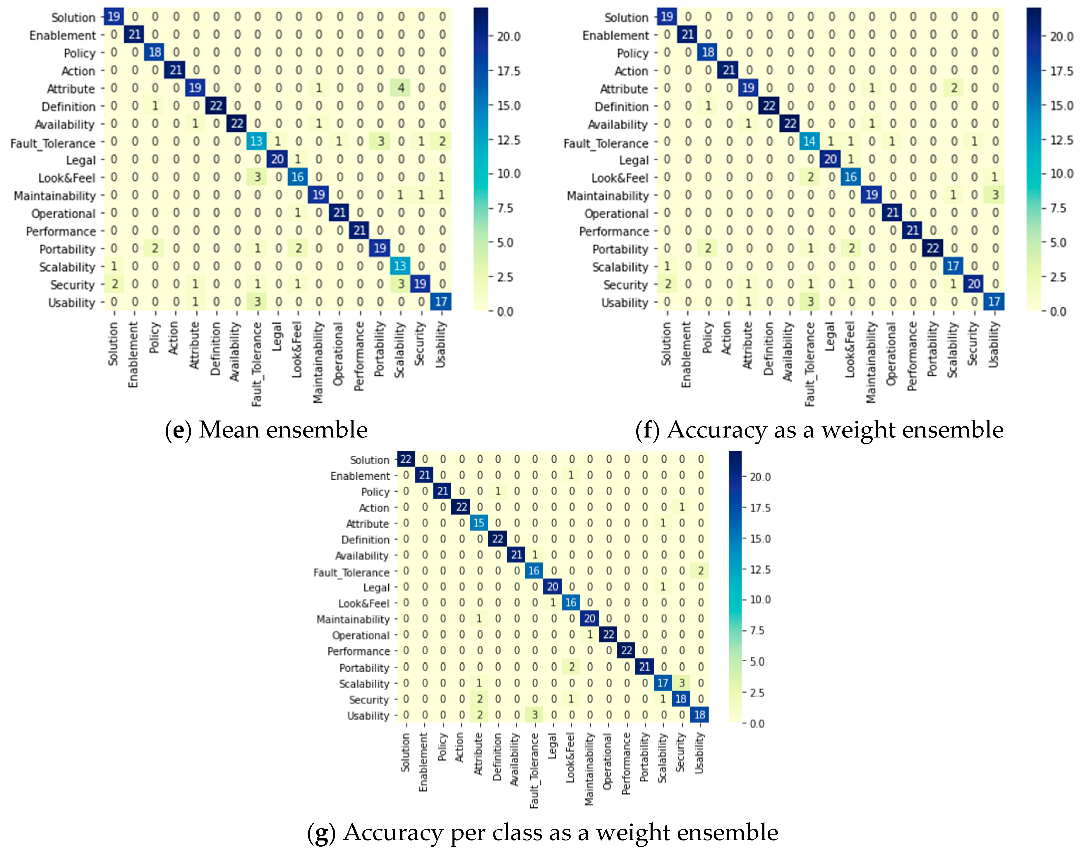
4.4.2. Multi-Class Classification Phase of NFRs and FRs into 17 Classes
- A.
- Training
- B.
- Test Results and discussion
4.4.3. All Together Two-Phase Classification System
5. Comparative Analysis
6. Conclusions and Future Work
Author Contributions
Funding
Data Availability Statement
Conflicts of Interest
References
- Tiun, S.; Mokhtar, U.A.; Bakar, S.H.; Saad, S. Classification of functional and non-functional requirement in software requirement using Word2vec and fast Text. J. Phys. Conf. Ser. 2020, 1529, 042077. [Google Scholar] [CrossRef]
- IEEE Standard Glossary of Software Engineering Terminology. In IEEE Std 729-1983; IEEE: Manhattan, NY, USA, 1990; pp. 1–84. [CrossRef]
- Canedo, E.D.; Mendes, B.C. Software requirements classification using machine learning algorithms. Entropy 2020, 22, 1057. [Google Scholar] [CrossRef] [PubMed]
- Alomari, R.; Elazhary, H. Implementation of a formal software requirements ambiguity prevention tool. Int. J. Adv. Comput. Sci. Appl. 2018, 9, 424–432. [Google Scholar] [CrossRef]
- Kurtanovic, Z.; Maalej, W. Automatically Classifying Functional and Non-functional Requirements Using Supervised Machine Learning. In Proceedings of the 2017 IEEE 25th International Requirements Engineering Conference (RE), Lisbon, Portugal, 4–8 September 2017; IEEE: Piscataway, NJ, USA, 2017; pp. 490–495. [Google Scholar]
- Del Carpio, A.F.; Angarita, L.B. Trends in Software Engineering Processes using Deep Learning: A Systematic Literature Review. In Proceedings of the 2020 46th Euromicro Conference on Software Engineering and Advanced Applications (SEAA), Portoroz, Slovenia, 26–28 August 2020; IEEE: Piscataway, NJ, USA, 2020; Volume 33, pp. 445–454. [Google Scholar]
- Navarro-Almanza, R.; Juarez-Ramirez, R.; Licea, G. Towards Supporting Software Engineering Using Deep Learning: A Case of Software Requirements Classification. In Proceedings of the 2017 5th International Conference in Software Engineering Research and Innovation (CONISOFT), Merida, Mexico, 25–27 October 2017; IEEE: Piscataway, NJ, USA, 2017; Volume 2018, pp. 116–120. [Google Scholar]
- Brownlee, J. Ensemble Learning Methods for Deep Learning Neural Networks. Available online: https://machinelearningmastery.com/ensemble-methods-for-deep-learning-neural-networks/ (accessed on 2 March 2021).
- Ott, D. Automatic Requirement Categorization of Large Natural Language Specifications at Mercedes-Benz for Review Improvements. In Proceedings of the 19th International Conference on Requirements Engineering: Foundation for Software Quality, ser. REFSQ, Essen, Germany, 8–11 April 2013; Springer: Berlin/Heidelberg, Germany, 2013; pp. 50–64. [Google Scholar]
- Winkler, J.; Vogelsang, A. Automatic Classification of Requirements Based on Convolutional Neural Networks. In Proceedings of the 2016 IEEE 24th International Requirements Engineering Conference Workshops (REW), Beijing, China, 12–16 September 2016; IEEE: Piscataway, NJ, USA, 2016; pp. 39–45. [Google Scholar]
- Rahimi, N.; Eassa, F.; Elrefaei, L. An Ensemble Machine Learning Technique for Functional Requirement Classification. Symmetry 2020, 12, 1601. [Google Scholar] [CrossRef]
- Slankas, J.; Williams, L. Automated extraction of non-functional requirements in available documentation. In Proceedings of the 2013 1st International Workshop on Natural Language Analysis in Software Engineering (NaturaLiSE), San Francisco, CA, USA, 25 May 2013; IEEE: Piscataway, NJ, USA, 2013; pp. 9–16. [Google Scholar] [CrossRef]
- Cleland-Huang, J.; Settimi, R.; Zou, X.; Solc, P. Automated classification of non-functional requirements. Requir. Eng. 2007, 12, 103–120. [Google Scholar] [CrossRef]
- Casamayor, A.; Godoy, D.; Campo, M. Identification of non-functional requirements in textual specifications: A semi-supervised learning approach. Inf. Softw. Technol. 2010, 52, 436–445. [Google Scholar] [CrossRef]
- Li, L.F.; Jin-An, N.C.; Kasirun, Z.M.; Piaw, C.Y. An Empirical comparison of machine learning algorithms for classification of software requirements. Int. J. Adv. Comput. Sci. Appl. 2019, 10, 258–263. [Google Scholar] [CrossRef]
- Casamayor, A.; Godoy, D.; Campo, M. Semi-Supervised Classification of Non-Functional Requirements: An Empirical Analysis. Intel. Artif. 2010, 13, 35–45. [Google Scholar] [CrossRef]
- Haque, M.A.; Rahman, M.A.; Siddik, M.S. Non-Functional Requirements Classification with Feature Extraction and Machine Learning: An Empirical Study. In Proceedings of the 1st International Conference on Advances in Science, Engineering and Robotics Technology 2019, Dhaka, Bangladesh, 3–5 May 2019. [Google Scholar]
- Fong, V. Software Requirements Classification Using Word Embeddings and Convolutional Neural Networks. Master’s Thesis, California Polytechnic State University, San Luis Obispo, CA, USA, June 2018. [Google Scholar]
- Hayes, J.; Li, W.; Rahimi, M. Weka meets TraceLab: Toward Convenient Classification: Machine Learning for Requirements Engineering Problems: A Position Paper. In Proceedings of the 2014 IEEE 1st International Workshop on Artificial Intelligence for Requirements Engineering (AIRE), Karlskrona, Sweden, 26 August 2014; IEEE: Piscataway, NJ, USA, 2014; pp. 9–12. [Google Scholar]
- Hey, T.; Keim, J.; Koziolek, A.; Tichy, W.F. NoRBERT: Transfer Learning for Requirements Classification. In Proceedings of the 28th IEEE International Conference on Requirements Engineering, Zurich, Switzerland, 31 August–4 September 2020. [Google Scholar]
- Zhang, K.; Liu, N.; Yuan, X.; Guo, X.; Gao, C.; Zhao, Z.; Ma, Z. Fine-Grained Age Estimation in the Wild with Attention LSTM Networks. In IEEE Transactions on Circuits and Systems for Video Technology; IEEE: Piscataway, NJ, USA, 2019; pp. 3140–3152. [Google Scholar] [CrossRef] [Green Version]
- Khayyat, M.M.; Elrefaei, L.A. Manuscripts Image Retrieval Using Deep Learning Incorporating a Variety of Fusion Levels. IEEE Access 2020, 8, 136460–136486. [Google Scholar] [CrossRef]
- Luo, L.; Yang, Z.; Lin, H.; Wang, J. Document triage for identifying protein-protein interactions affected by mutations: A neural network ensemble approach. Database 2018, 2018, bay097. [Google Scholar] [CrossRef] [PubMed]
- Nguyen, V.Q.; Anh, T.N.; Yang, H.-J. Real-time event detection using recurrent neural network in social sensors. Int. J. Distrib. Sens. Netw. 2019, 15, 155014771985649. [Google Scholar] [CrossRef] [Green Version]
- Pan, M.; Zhou, H.; Cao, J.; Liu, Y.; Hao, J.; Li, S.; Chen, C.H. Water Level Prediction Model Based on GRU and CNN. IEEE Access 2020, 8, 60090–60100. [Google Scholar] [CrossRef]
- Shahid, F.; Zameer, A.; Muneeb, M. Predictions for COVID-19 with deep learning models of LSTM, GRU and Bi-LSTM. Chaos Solitons Fractals 2020, 140, 110212. [Google Scholar] [CrossRef] [PubMed]
- Demir, N. Ensemble Methods: Elegant Techniques to Produce Improved Machine Learning Results. Available online: https://www.toptal.com/machine-learning/ensemble-methods-machine-learning (accessed on 10 October 2020).
- Brownlee, J. What is a Confusion Matrix in Machine Learning? Available online: https://machinelearningmastery.com/confusion-matrix-machine-learning/ (accessed on 1 October 2020).
- Baccouche, A.; Garcia-Zapirain, B.; Olea, C.C.; Elmaghraby, A. Ensemble deep learning models for heart disease classification: A case study from Mexico. Information 2020, 11, 207. [Google Scholar] [CrossRef] [Green Version]
- Jethwani, T. Difference Between Categorical and Sparse Categorical Cross Entropy Loss Function. Available online: https://leakyrelu.com/2020/01/01/difference-between-categorical-and-sparse-categorical-cross-entropy-loss-function/ (accessed on 11 November 2020).
- Harikrishnan, N.B. Confusion Matrix, Accuracy, Precision, Recall, F1 Score. Available online: https://medium.com/analytics-vidhya/confusion-matrix-accuracy-precision-recall-f1-score-ade299cf63cd (accessed on 28 May 2021).
- Brownlee, J. Random Oversampling and Undersampling for Imbalanced Classification. Available online: https://machinelearningmastery.com/random-oversampling-and-undersampling-for-imbalanced-classification/ (accessed on 5 June 2021).


| Class | Definition | Example |
|---|---|---|
| Solution | Includes actions that are expected to be carried out by the system or different users. | “The system shall display completed worklist items to the Lab Manager.” |
| Enablement | Includes the capabilities offered by the system to different users. Subsystems that offer these capabilities are optionally specified. | “The Lab Manager shall be able to create worklist items.” |
| Attribute Constraint | Constraints on attributes or entity attributes are specified through this class. | “Search options must always be one of the following: Price, destination, restaurant type, or specific dish.” |
| Action Constraint | Allowed and non-allowed actions by the system or the subsystems displayed using this class. | “The loan subsystem may only delete a lender if there are no loans in the portfolio associated with this lender.” |
| Policy | This class is responsible for specifying all policies that have been decided for the system. | “A loan is not computed in more than one bundle.” |
| Definition | All entities are defined using this class. | “The expected profit of a fixed-rate loan is defined as the amount of interest received over the remaining life of the loan.” |
| Class | Definition | Example |
|---|---|---|
| Availability | Related to users’ accessibility to a system at a specific time. | “The product shall be available 24 h per day, seven days per week.” |
| Fault Tolerance | Determines the degree to which the system or product operates in the absence of hardware or software faults. | “100% of saved user preferences shall be restored when the system comes back online.” |
| Legal and Licensing | Determines the licenses and certificates that the system needs to obtain. | “All actions that modify an existing dispute case must be recorded in the case history.” |
| Look and Feel | Specifies the appearance and style. | “The website design should be modern, clean, and concise.” |
| Maintainability | Effectiveness and efficiency of a system modified by maintainers. | “Application updates shall occur between 3:00 a.m. and 6:00 a.m. CST on Wednesday morning during the middle of the NFL season.” |
| Operability | How easy to operate and control a system through its attributes. | “The product shall run on the existing hardware for all environments.” |
| Performance | Related to required resources at a specific condition. | “A customer shall be able to check the status of their prepaid card by entering in the PIN number in under 5 s.” |
| Portability | The effectiveness and efficiency in transferring the system from one hardware, software, or environment to another. | “The product is expected to run on Windows CE and Palm operating systems.” |
| Scalability | The degree to which a system adapts effectively and efficiently from one hardware, software, or environment to another. | “The system shall be able to handle all of the user requests/usage during business hours.” |
| Security | Includes the protection of personal data and authorized access. | “The product shall provide authentication and authorization.” |
| Usability | The level of efficiency and effectiveness of a system that can be used by specific users to reach specific goals with satisfaction. | “The product shall be installed by an untrained realtor without recourse to separately printed instructions.” |
| Reference # Year | Classification | Methodology | Dataset | Results | Advantages | Disadvantages | |
|---|---|---|---|---|---|---|---|
| Input | Classes | ||||||
| 1. Classifying SRs into Main Classes | |||||||
| [9] 2013 | Software requirements (SRs) | Topics | Support Vector Machine (SVM) and Multinomial Naïve Bayes (MNB) | Two German specifications by Mercedes-Benz (public and confidential) | Recall: 0.94 (MNB) Precision: 0.86 (SVM) | Reliable results. Improves technical review to enhance SRs. | No enough training data. |
| [10] 2017 | Text | Requirement OR Information | Convolutional Neural Network (CNN) | DOORS document database | Accuracy: 81% Precision: 0.73 Recall: 0.89 | One of the first studies that used CNN. | Does not point to wrongly classified input. |
| 2. Classifying FRs into Multi-Classes | |||||||
| [11] 2020 | Functional requirements (FRs) | Solution Enablement Action constraint Attribute constraint Definition Policy | Ensemble (accuracy per class as a weight) includes support vector classification, support vector machine, decision tree, logistic regression, and naïve Bayes | Collected dataset that has 600 FR statements with 100 FRs from each category | Accuracy: 99.45% Time: 0.07 s | Novel ensemble approach. New introduced FR dataset. | Limited to FRs. |
| 3. Classifying Non-Functional Requirements (NFRs) into Multi-Classes | |||||||
| [7] 2017 | SRs | Functional Availability Legal Look and feel Maintainability Operational Performance Scalability Security Usability Fault tolerance Portability | CNN | PROMISE corpus | Precession: 0.80 Recall: 0.785 F-measure: 0.77 | SRs classified into 12 classes using DL. SRs prepared simply using the proposed reprocessing method. DL evaluated to support RE. | Limited to CNN only, while other models could be used. |
| [18] 2018 | 1. SRs 2. NFRs 3. NFRs | 1. FRs NFRs 2. Availability Legal Maintainability Operational Performance Scalability Look and feel Security usability 3. Security Not Security | CNN | PROMISE corpus | 1. F1 score: 0.945 2. F1 score: 0.911 3. F1 score: 0.772 | Utilizing word embedding in vectorization leads to improvement in SR classification. | Various aspects unexplored in the method and validation. |
| [19] 2014 | SRs | FR Access control Person authentication Security encryption Decryption Audit control Automatic Logoff Integrity controls Unique user Identification Transmission Encryption Decryption Emergency Access procedure Transmission Security | WekaClassifiersTrees REPTree J48 | Certification Commission for Healthcare Information Technology (CCHIT) dataset | Accuracy: 93.92% | ML algorithms combined to solve 2 RE problems, and more problems can be solved. | Additional components required to solve RE problems with Tracelab. |
| [12] 2013 | NFRs | 14 NFR classes such as: Capacity Reliability Security | K-nearest neighbor classifier | 11 documents related to electronic health records (EHRs) | F1: 0.54 | Ability to extract relevant NFRs from documents. | Limited to NFRs. Specific data field. |
| [13] 2007 | SR | FRs Availability Look and-feel legal Maintainability Operational Performance Scalability Security Usability | Classification based on key words for each category, along with finding the weight based on frequency for each keyword used by TF-IDF | Labeled 326 NFRs and 358 FRs from 15 different projects | Considering only the top 15 keywords for each category scored the highest Recall: 0.7669 | Provided an incremental approach for training a classifier in new domains. | More efforts to improve stopping conditions. Run time needs to be improved to be used by a real analyst. |
| [14] 2010 | SR | FRs Availability Look and feel Legal Maintainability Operational Performance Scalability Security Usability | Naïve Bayes classifier | Labeled 326 NFRs and 358 FRs from 15 different projects | Accuracy: 97% | Feasibility of using semi-supervised learning in NFR classification. | Dataset is limited to the top-ranked examples. |
| [15] 2019 | SR | FRs NFRs categorized into 10 categories such as: Security Performance Usability | Ensemble method consists of random forest and gradient boosting | Text files in a format of SQL and CSV files | NFR accuracy: 0.826 (gradient boosting) FR accuracy: 0.591 (random forest) | Highly accurate algorithms for SR classification. | Limited study due to limited data. Could not determine the number of SRs in a sentence. Could not read input from .docx and .txt files. |
| [16] 2010 | SR | FRs NFRs categorized into categories such as: Security Availability Scalability | Naïve Bayes classifier | Collected SRs by interviews and other methods (255 FRs, NFRFR range from 10 to 67 per category) | NFR precision: 75% | Reduced manual labeling efforts. | Limited to NFR multi-class classification |
| [17] 2019 | SR | FRs Availability Legal Look and feel Maintainability Operational Performance Scalability Security Usability Fault tolerance Portability | Multinomial naïve Bayes (MNB) Gaussian naïve Bayes (GNB) Bernoulli naïve Bayes (BNB) K-nearest neighbor (KNN) Support vector machine (SVM) Stochastic gradient descent SVM (SGD SVM) Decision tree (Dtree) | PROMISE dataset (625 requirement sentences: 255 FRs and 370 NFRs) | Precision: 0.66 Recall: 0.61 F1 score: 0.61 Accuracy: 0.76 Using SGD SVM classifier and TF-IDF for feature extraction | Seven algorithms used. | Need to apply other classification techniques such as boosting and bagging. |
| 4. Complete System (Classifying NFRs and FRs into Multi-Classes) | |||||||
| [20] 2020 | 1. SRs 2. NFRs 3. FRs | 1. FRs NFRs 2. Usability Security Operational Performance 3. Functions Data Behavior | Fine-tuned BERT (NoRBERT) | PROMISE | 1. F1 score: 90% FRs and 93% NFRs 2. F1 score: 76% 3. F1 score: 92% | Novelty in FR classification. Modern algorithm used with transfer learning. | Multi-class or multi-label classification for FRs not considered. |
| Classes | Number of Statements |
|---|---|
| Availability (A) | 29 |
| Fault tolerance (FT) | 12 |
| Legal (L) | 14 |
| Look and feel (LF) | 42 |
| Maintainability (MN) | 17 |
| Operational (O) | 68 |
| Performance (PE) | 54 |
| Portability (PO) | 2 |
| Scalability (SC) | 21 |
| Security (SE) | 67 |
| Usability (US) | 67 |
| FRs | 266 |
| Total | 659 |
| FR Classes | Number of Statements |
|---|---|
| Policy (P) | 41 |
| Solution (S) | 116 |
| Enablement (E) | 71 |
| Action constraint (AC) | 25 |
| Attribute constraint (AT) | 7 |
| Definition (D) | 6 |
| Total | 266 |
| Layer | Output Shape | Number of Parameters |
|---|---|---|
| Embedding_64 | (None, None, 46) | 77,280 |
| Spatial_dropout1d_39 | (None, None, 46) | 0 |
| Bidirectional_39 | (None, 92) | 34,224 |
| Dense_149 | (None, 46) | 4278 |
| Dropout_95 | (None, 46) | 0 |
| Dense_150 | (None, 46) | 2162 |
| Dropout_96 | (None, 46) | 0 |
| Dense_151 | (None, 17) | 799 |
| Activation_39 | (None, 17) | 0 |
| Layer | Output Shape | Number of Parameters |
|---|---|---|
| Embedding_65 | (None, None, 46) | 77,280 |
| Dropout_97 | (None, None, 46) | 0 |
| Conv1d_10 | (None, None, 46) | 6394 |
| Global_max_pooling1d_10 | (None, 46) | 0 |
| Dense_152 | (None, 128) | 6016 |
| Dropout_98 | (None, 128) | 0 |
| Dense_153 | (None, 17) | 2193 |
| Layer | Output Shape | Number of Parameters |
|---|---|---|
| Embedding_66 | (None, None, 46) | 77,280 |
| Gru_17 | (None, None, 46) | 12,834 |
| Gru_18 | (None, 32) | 7584 |
| Dense_154 | (None, 17) | 561 |
| Layer | Output Shape | Number of Parameters |
|---|---|---|
| Embedding_67 | (None, None, 46) | 77,280 |
| Lstm_56 | (None, None, 46) | 17,112 |
| Lstm_57 | (None, 32) | 10,112 |
| Dense_155 | (None, 17) | 561 |
| DL Models | Accuracy (%) | Precision | Recall | F1 Score |
|---|---|---|---|---|
| BiLSTM | 84.022 | 0.84 | 0.85 | 0.84 |
| LSTM | 74.656 | 0.75 | 0.74 | 0.72 |
| CNN | 91 | 0.92 | 0.92 | 0.92 |
| GRU | 78.78 | 0.79 | 0.79 | 0.78 |
| Mean ensemble | 88.15 | 0.88 | 0.89 | 0.88 |
| Accuracy as a weight ensemble | 90.63 | 0.91 | 0.91 | 0.91 |
| Accuracy per class as a weight | 92.56 | 0.93 | 0.93 | 0.93 |
| Layer | Output Shape | Number of Parameters |
|---|---|---|
| Embedding_68 | (None, None, 46) | 60,858 |
| Spatial_dropout1d_40 | (None, None, 46) | 0 |
| Bidirectional_40 | (None, 92) | 34,224 |
| Dense_156 | (None, 46) | 4278 |
| Dropout_99 | (None, 46) | 0 |
| Dense_157 | (None, 46) | 2162 |
| Dropout_100 | (None, 46) | 0 |
| Dense_158 | (None, 3) | 141 |
| Activation_40 | (None, 3) | 0 |
| Layer | Output Shape | Number of Parameters |
|---|---|---|
| Embedding_69 | (None, None, 46) | 60,858 |
| Dropout_101 | (None, None, 46) | 0 |
| Conv1d_11 | (None, None, 46) | 6394 |
| Global_max_pooling1d_11 | (None, 46) | 0 |
| Dense_159 | (None, 128) | 6016 |
| Dropout_102 | (None, 128) | 0 |
| Dense_160 | (None, 2) | 258 |
| Layer | Output Shape | Number of Parameters |
|---|---|---|
| Embedding_70 | (None, None, 46) | 60,858 |
| Gru_19 | (None, None, 46) | 12,834 |
| Gru_20 | (None, 32) | 7584 |
| Dense_161 | (None, 2) | 66 |
| Layer | Output Shape | Number of Parameters |
|---|---|---|
| Embedding_71 | (None, None, 46) | 60,858 |
| Lstm_59 | (None, None, 46) | 17,112 |
| Lstm_60 | (None, 32) | 10,112 |
| Dense_162 | (None, 2) | 66 |
| DL Models | Accuracy (%) | Precision | Recall | F1 Score |
|---|---|---|---|---|
| BiLSTM | 95.00 | 0.94 | 0.95 | 0.94 |
| LSTM | 93.22 | 0.93 | 0.93 | 0.93 |
| CNN | 93.22 | 0.93 | 0.94 | 0.93 |
| GRU | 92.37 | 0.92 | 0.92 | 0.92 |
| Mean ensemble | 94.4 | 0.94 | 0.95 | 0.94 |
| Accuracy as a weight ensemble | 94.9 | 0.95 | 0.95 | 0.95 |
| Accuracy per class as a weight ensemble | 96 | 0.96 | 0.96 | 0.96 |
| Layer | Output Shape | Number of Parameters |
|---|---|---|
| Embedding_8 | (None, None, 46) | 28,106 |
| Spatial_dropout1d_3 | (None, None, 46) | 0 |
| Bidirectional_3 | (None, 92) | 34,224 |
| Dense_14 | (None, 46) | 4278 |
| Dropout_9 | (None, 46) | 0 |
| Dense_15 | (None, 46) | 2162 |
| Dropout_10 | (None, 46) | 0 |
| Dense_16 | (None, 6) | 282 |
| Activation_3 | (None, 6) | 0 |
| Layer | Output Shape | Number of Parameters |
|---|---|---|
| Embedding_9 | (None, None, 46) | 28,106 |
| Dropout1d_11 | (None, None, 46) | 0 |
| Conv1d_3 | (None, None, 46) | 6394 |
| Global_max_pooling1d_3 | (None, 46) | 0 |
| Dense_17 | (None, 128) | 6016 |
| Dropout_12 | (None, 128) | 0 |
| Dense_18 | (None, 6) | 774 |
| Layer | Output Shape | Number of Parameters |
|---|---|---|
| Embedding_10 | (None, None, 46) | 28,106 |
| GRU_5 | (None, None, 46) | 12,834 |
| GRU_6 | (None, 32) | 7584 |
| Dense_19 | (None, 6) | 198 |
| Layer | Output Shape | Number of Parameters |
|---|---|---|
| Embedding_11 | (None, None, 46) | 28,106 |
| Lstm_6 | (None, None, 46) | 17,112 |
| Lstm_7 | (None, 32) | 10,112 |
| Dense_20 | (None, 6) | 198 |
| Layer | Output Shape | Number of Parameters |
|---|---|---|
| Embedding_4 | (None, None, 46) | 53,958 |
| Spatial_dropout1d_4 | (None, None, 46) | 0 |
| Bidirectional_4 | (None, 92) | 34,224 |
| Dense_21 | (None, 46) | 4278 |
| Dropout_13 | (None, 46) | 0 |
| Dense_22 | (None, 46) | 2162 |
| Dropout_14 | (None, 46) | 0 |
| Dense_23 | (None, 11) | 517 |
| Activation_4 | (None, 11) | 0 |
| Layer | Output Shape | Number of Parameters |
|---|---|---|
| Embedding_13 | (None, None, 46) | 53,958 |
| Dropout_15 | (None, None, 46) | 0 |
| Conv1d_4 | (None, None, 46) | 6394 |
| Global_max_pooling1d_4 | (None, 46) | 0 |
| Dense_24 | (None, 128) | 6016 |
| Dropout_16 | (None, 128) | 0 |
| Dense_25 | (None, 11) | 1419 |
| Layer | Output Shape | Number of Parameters |
|---|---|---|
| Embedding_14 | (None, None, 46) | 53,958 |
| GRU_7 | (None, None, 46) | 12,834 |
| GRU_8 | (None, 32) | 7584 |
| Dense_26 | (None, 11) | 363 |
| Layer | Output Shape | Number of Parameters |
|---|---|---|
| Embedding_15 | (None, None, 46) | 53,958 |
| Lstm_9 | (None, None, 46) | 17,112 |
| Lstm_10 | (None, 32) | 10,112 |
| Dense_27 | (None, 11) | 363 |
| DL Models | Accuracy (%) | Precision | Recall | F1 Score |
|---|---|---|---|---|
| BiLSTM | 96.8 | 0.97 | 0.97 | 0.97 |
| LSTM | 78.91 | 0.79 | 0.79 | 0.79 |
| CNN | 96.0 | 0.96 | 0.96 | 0.96 |
| GRU | 58.59 | 0.59 | 0.59 | 0.59 |
| Mean ensemble | 96.8 | 0.97 | 0.97 | 0.97 |
| Accuracy as a weight ensemble | 96.8 | 0.97 | 0.97 | 0.97 |
| Accuracy per class as a weight ensemble | 98 | 0.98 | 0.98 | 0.98 |
| DL Models | Accuracy (%) | Precision | Recall | F1 Score |
|---|---|---|---|---|
| BiLSTM | 83.7 | 0.84 | 0.85 | 0.84 |
| LSTM | 63.0 | 0.64 | 0.63 | 0.64 |
| CNN | 83.3 | 0.83 | 0.83 | 0.83 |
| GRU | 56.0 | 0.57 | 0.56 | 0.55 |
| Mean ensemble | 85.0 | 0.85 | 0.84 | 0.85 |
| Accuracy as a weight ensemble | 85.1 | 0.85 | 0.85 | 0.85 |
| Accuracy per class as a weight | 86.5 | 0.89 | 0.86 | 0.87 |
| DL Models | Average Accuracy (%) | Average Precision | Average Recall | Average F1 Score |
|---|---|---|---|---|
| BiLSTM | 91.66 | 0.91 | 0.92 | 0.91 |
| LSTM | 78.37 | 0.78 | 0.78 | 0.78 |
| CNN | 90.84 | 0.90 | 0.91 | 0.90 |
| GRU | 68.98 | 0.69 | 0.69 | 0.68 |
| Mean ensemble | 92.06 | 0.92 | 0.92 | 0.92 |
| Accuracy as a weight ensemble | 92.26 | 0.92 | 0.92 | 0.92 |
| Accuracy per class as a weight | 93.4 | 0.94 | 0.93 | 0.93 |
| Reference # | Classification | Methodology | Dataset | Results | |
|---|---|---|---|---|---|
| Year | Input | Classes | |||
| 1. Classifying NFRs into Multi-Classes | |||||
| [7] 2017 | SRs | Functional Availability | CNN | PROMISE corpus | Precession: 0.80 |
| Legal | Recall: 0.785 | ||||
| Look and feel Maintainability Operational | F measure: 0.77 | ||||
| Performance Scalability | |||||
| Security | |||||
| Usability | |||||
| Fault tolerance Portability | |||||
| [18] 2018 1. SR 2. NFRs 3. NFRs | 1. FRs NFRs 2. Availability Legal Maintainability Operational Performance Scalability Look and feel Security Usability 3. Security Non-security | CNN | PROM corpus | 1. F1 score: 0.945 2. F1 score: 0.911 3. F1 score: 0.772 | |
| [17] 2019 | SRs | FR Availability Legal Look and feel Maintainability Operational Performance Scalability Security Usability Fault tolerance Portability | Multinomial naïve Bayes (MNB) Gaussian naïve Bayes (GNB) Bernoulli naïve Bayes (BNB) K-nearest neighbor (KNN) Support vector machine (SVM) Stochastic gradient descent SVM (SGD SVM) Decision tree (Dtree) | PROMISE dataset | Precision: 0.66 Recall: 0.61 F1 score: 0.61 Accuracy: 0.76 Using the SGD SVM classifier and TF-IDF for feature extraction |
| 2. Complete System (classifying NFRs and FRs into Multi-Classes) | |||||
| [20] 2020 | 1. SRs 2. NFRs 3. FRs | 1. FRs–NFRs 2. Usability Security Operational Performance 3. ions Data behavior | Fine-tuned BERT (NoRBERT) | PROMISE | 1. F1 Score: 90% FRs and 93% NFRs 2. F1 Score: 76% 3. F1 Score: 92% |
| 2021 Proposed one-phase classification system | SRs | 17 classes of FRs and NFRs (6 classes of FRs and 11 classes of NFRs) | Ensemble DL-based model (BiLSTM-LSTM-CNN-GRU) | PROMISE | Accuracy: 92.56% Precision: 0.93 Recall: 0.93 F1 Score: 0.93 |
| 2021 Proposed two-phase classification system | SRs | 1. Phase one: Binary classification into FRs or NFRs 2. Phase two: Multi-class classification of FRs (6 classes) and NFRs (11 classes) | Ensemble DL-based model (BiLSTM–LSTM–CNN–GRU) | PROMISE | 1.Accuracy: 95.7% Precision: 0.96 Recall: 0.96 F1 Score: 0.96 2. Accuracy: 93.4% Precision: 0.94 Recall: 0.93 F1 Score: 0.93 |
Publisher’s Note: MDPI stays neutral with regard to jurisdictional claims in published maps and institutional affiliations. |
© 2021 by the authors. Licensee MDPI, Basel, Switzerland. This article is an open access article distributed under the terms and conditions of the Creative Commons Attribution (CC BY) license (https://creativecommons.org/licenses/by/4.0/).
Share and Cite
Rahimi, N.; Eassa, F.; Elrefaei, L. One- and Two-Phase Software Requirement Classification Using Ensemble Deep Learning. Entropy 2021, 23, 1264. https://doi.org/10.3390/e23101264
Rahimi N, Eassa F, Elrefaei L. One- and Two-Phase Software Requirement Classification Using Ensemble Deep Learning. Entropy. 2021; 23(10):1264. https://doi.org/10.3390/e23101264
Chicago/Turabian StyleRahimi, Nouf, Fathy Eassa, and Lamiaa Elrefaei. 2021. "One- and Two-Phase Software Requirement Classification Using Ensemble Deep Learning" Entropy 23, no. 10: 1264. https://doi.org/10.3390/e23101264
APA StyleRahimi, N., Eassa, F., & Elrefaei, L. (2021). One- and Two-Phase Software Requirement Classification Using Ensemble Deep Learning. Entropy, 23(10), 1264. https://doi.org/10.3390/e23101264