1. Introduction
Phase transition, which qualitatively characterizes the change in the state of a system under a continuous change in an external parameter, is ubiquitously found in probabilistic models and statistical mechanics. In this paper, we investigate the phase transitions in the Finitary Random Interlacement (FRI) introduced by Bowen in his study on Gaboriau–Lyons problem [
1]. In contrast to its profound connection with the von Neumann–Day problem, a relatively simple description of FRI is given by Bowen in [
1] as follows: Consider a random network
in
. For each vertex
, there lives
frogs, where
is a Poisson random variable with mean
,
is the degree of
x and
are two positive parameters. Each frog has a coin that lands on head with probability
. At time
, the frog flips the coin. If it lands on heads, the frog moves to a random neighboring vertex with equal probability. It repeats this operation until the coin lands on tails, at which point the frog stops forever. The FRI is the random multiset of random walk paths of all frogs. It is worth noting that
u gives a natural parameterization of the ”vertex intensity“ of the FRI, as it is proportional to the expected number of vertices visited by all frogs starting from each given point.
Since each path consists of a simple random walk for
t steps and a geometric random variable with mean
at
steps, a FRI can be roughly treated as a random network
in
“interlaced” by fibers made of geometrically truncated simple random walk (SRW) trajectories, with a multiplicative parameter
u controlling its Poisson intensity and truncation parameter
T that determines the expected length of each fiber. As pointed out by an anonymous referee (of a previous paper), an FRI can also be described as a variant of the Random Interlacement (RI) [
2] in
with weight [
3], determined by capacity with a discrete killing measure [
4]. See
Section 2 for more precise definitions and constructions for FRI.
In the following, we denote by
the FRI in
with multiplicative parameter
u and truncation parameter
T, which is the collection of edges traversed by ”fibers“ in a Poisson point process. See
Section 2.1 for details. A key character of the FRI is percolation property, i.e., the existence and uniqueness of an infinite cluster within
. In contrast to RI, where
almost surely percolates for all
d and
, FRI has been proved in [
5] to have the following phase transition as an edge percolation model:
Supercritical phase (Theorem 1, [
5]): for all
and
, there is a
such that for all
,
almost surely percolates.
Subcritical phase (Theorem 2, [
5]): for all
and
, there is a
such that for all
,
has no infinite cluster almost surely.
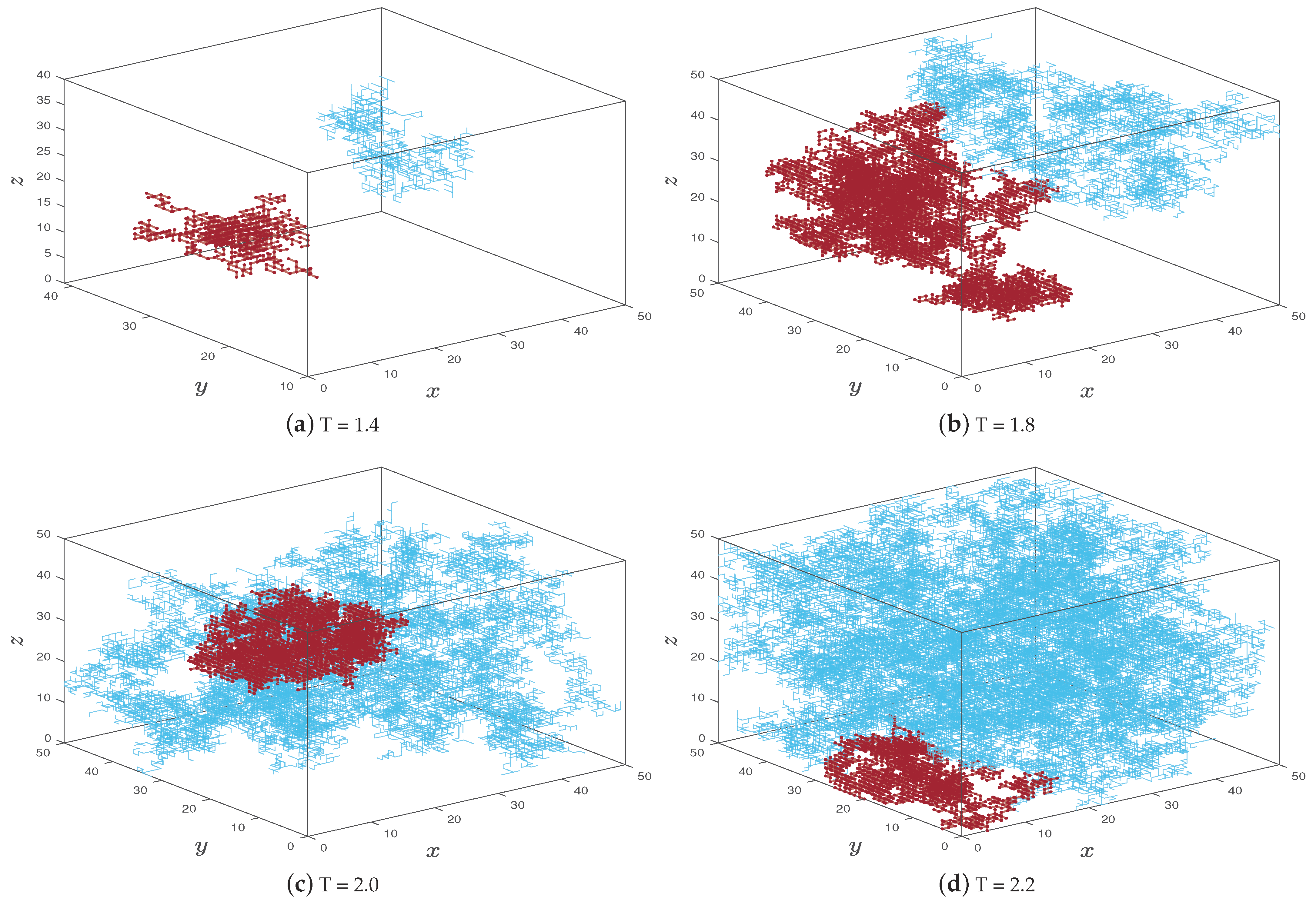
Intuitively, the percolation can be visualized by running one realization under different parameters
and plotting the first and second largest clusters restricted in a finite box
. Two small clusters in
Figure 1a, that corresponds to
, provide some evidence that no infinite cluster exists, while a huge cluster along with a smaller cluster in
Figure 1d that corresponds to
indicates that there may exist only one infinite cluster. One can see that the phase transition may occur near
, in which the first and second largest clusters are almost of the same size. The dominance of the first largest cluster can be apparently observed as
T becomes larger, e.g.,
.
Moreover, a follow-up work [
6] proved recently that for all
and
, there is a
such that for all
, the chemical distance on
is asymptotically of the same order as the Euclidean distance. Reference [
6] further proves that FRI has local uniqueness property for all sufficiently large
T. See [
7] for precise definitions for chemical distance and local uniqueness. However, since
may be nonmonotonic with respect to
T, the existence of a subcritical and a supercritical phase is insufficient to guarantee a critical value in between. It is conjectured in [
5] that there is a unique critical value
such that
percolates when
and has no infinite cluster almost surely when
.
The percolation phase transition is closely related to the trade-off mechanism with respect to the parameter
T: As
T increases, there will be on average fewer and fewer fibers starting from each vertex. In compensation however, the length of each remaining fiber increases proportionally to
T, so that we are less likely to see the start or end of any fiber locally. In fact, as
, an FRI increasingly resembles the limiting model (which is the classical RI itself) where all fibers are doubly infinite SRW trajectories. It has been proved in [
1] that
under the weak-* topology. With the observation above, it is natural to ask how the FRI, as a random collection of edges, evolves with respect to
T, or more specifically, whether or not it has stochastic monotonicity [
5].
Like random interlacement, FRI is by definition monotonically increasing with respect to its intensity u. In contrast, it is shown in the paper that for all , the set of edges covered by an is NOT stochastically monotone in T for . This reveals that the evolution of FRI with respect to T might be more nontrivial than previously thought, and makes the characterization of the phase diagram of T a more interesting question.
The nonmonotonicity of FRI casts shadows on the conjecture of existence and uniqueness of critical value . A large-scale parallel computing algorithm is employed to explore the behavior of FRI when the fiber length factor T changes in the interval . Our numerical findings strongly suggest that, although no longer monotonic, for any , still has a unique critical value of percolation. For the shape of the phase diagram, we prove that has to be the correct asymptotic order of as , given that the critical value exists; i.e., we find that there are , such that for all sufficiently large u
has no infinite cluster for all ;
has a unique infinite cluster for all .
Moreover, for all small u, we prove that has a polynomial upper bound with respect to u such that for all
when , ;
when , .
At the same time, our numerical tests also indicate that the phase diagram is inversely proportional to u.
The rest of this paper is outlined as follows: in
Section 2, we recall the precise definition of FRI, together with some important notations and constructions crucial for our theoretical and numerical discussions; in
Section 3 we discuss the nonmonotonicity of the edge set of FRI; in
Section 4, we discuss theoretical results about characterization of of phase diagram; our numerical explorations on the phase diagram are presented in
Section 5.
2. Definitions and Notations
In this section, we recall the precise definition of FRI, together with some important notations and constructions in [
1,
5,
6]. We start with some standard notations for simple random walks. Without causing further confusion, we will use
to denote both vertices and (the nearest neighbor) edges in the
dimensional lattice throughout this paper. Then, for a subgraph
, we call it connected if any
can be connected by a collection of edges in
E. For
, let
satisfy
,
. Denote the edges
and
by
and
. Note that
form the basis of
. For any subset of vertices
, let
be the inner and outer boundary of
A. We let
be the
box in
centered at
x of radius
n, i.e.,
Moreover, we abbreviate by .
In this paper, we denote by a simple random walk (SRW) in starting from , with its distribution denoted by . Note that for any integer , the SRW trajectory naturally induces a collection of edges . Moreover, for any , let be a geometric random variable with which is independent to . Then we call a geometrically killed SRW with parameter T, and denote its distribution by with the convention .
Moreover, we denote by
the first hitting and first returning times to
A, with the convention
.
Remark 1. It is worth noting that when .
For a finite subset
A and vertex
, define the killed escape probability
together with the killed equilibrium measure
and the killed capacity
We also abbreviate , , , , and to , , , , and , respectively, when .
Remark 2. Factor in the killed equilibrium measure is added for technical reasons to make FRI converge to RI with the same intensity as . See [1] for details. It is worth noting that for
,
2.1. Definition of FRI
According to [
5], there are two equivalent definitions of the Poisson point process corresponding to FRI. Denote the set of all finite paths on
by
. Since
is countable, the measure
is a
finite measure on
.
Definition 1. For , the finitary random interlacements is a Poisson point process on with intensity measure . The law of is denoted by .
Definition 2. For each site , is a Poisson random variable with parameter . Start independent geometrically killed simple random walks starting at x with killing rate . Then, one may equivalently define as a point measure on composed of all the trajectories above from all sites in .
With the Poisson point process defined as above, we define as the collection of all edges traversed by , which is a random subset of edges in .
2.2. Configurations within a Finite Set
In fact, given a finite set
, the distribution of FRI within
K can be described precisely. By Lemma 2.2 of [
5], if we start
independent random walks with distribution
for any
(denote all these trajectories by
), then
has the same distribution as
.
2.3. Stochastic Dominance and Monotonicity
A sufficient condition for the existence of the critical value is the stochastic monotonicity with respect to T. More precisely, if for any there is a coupling between and such that almost surely, then must exist. Therefore, we need the concept of stochastic dominance to describe the existence of the coupling.
Definition 3 (Definition 2.1, Chapter 2 of [
8]).
Assume that X is a compact metric space with a given partial order. Say a function f on X is monotone if for any , . Then, for two probability measures on X, say stochastically dominates (written by ) if and only if for any monotone function f on X, By Theorem 2.4 in the Chapter 2 of [
8], we know that the coupling mentioned above exists if and only if
.
3. Nonmonotonicity and Single Edge Density
In this section, we first show that unlike the Random Interlacement, an FRI is not stochastically monotone in
T for all
and
. The following proof was taught to us by an anonymous referee. Recalling the definition of stochastic monotonicity, to prove/disprove
for all
, it is equivalent to verify whether or not for all monotonically increasing functions
on
, one always has
In particular, we can first take the test function as the very simple form as follows: for each integer
, define
i.e.,
stands for the event where at least one edge in
E traverses
.
Theorem 1. For any , , FRI does not have stochastic monotonicity with respect to T.
Proof. Recalling the definition of
, one may define
to be the event that the FRI fails to intersect
. It now suffices to prove that for any
and
there exists
and
such that
Recalling (
3) and the construction in
Section 2.3, we have for all
,
Thus, we only need to show that
□
The proof of (
6) is based on the following well-known estimate on the capacity of a box:
Lemma 1 (Proposition
in [
9]).
There are constants such that for all , Note that
, then, there is a
such that
. At the same time, by (
4)
With Theorem 1, one may also consider the evolution of the FRI density for varying
T’s. Let
and thus the ”single edge density“
gives the probability that any single (undirected) edge is traversed by the FRI. By translation invariance,
is proportional to the expectation of the number of edges traversed by FRI within a given set. The following proposition shows that the density of and FRI is not monotone in
T for
, but becomes monotonically increasing for higher dimensions.
Proposition 1. For any , . Moreover, there are and such that
for any , for all ;
for , for all ;
there exists such that for all and .
Remark 3. As a direct corollary of Theorem 1 and Proposition 1, one may see that, for sufficiently large d, FRI is not monotone as well with respect to its edge density. We expect this should also hold for all .
Before presenting the proof of Proposition 1, we first cite the following useful result directly from Exercise 11.1 [
9] on the expected length of excursion given a SRW that returns to where it starts.
Lemma 2 (from Exercise 11.1, [
9]).
Suppose and is a simple random walk in with and let . Then, We also need a ”high dimensional“ version of Lemma 2. The main technicalities involved in the proof are asymptotic estimates for high-dimensional SRW’s, which are not directly related to the main scope of this paper, so we leave it in
Appendix A.
Lemma 3. Then, .
Now we are able to prove Proposition 1.
Proof of Proposition 1. We denote the event
by
F and then calculate
. First, we need to calculate
and
. Denote that
and
. We have
Restricted on
, there are
independent trajectories starting from 0 and
trajectories starting from 1. Note that
, we have
Let
and
. We have
Meanwhile,
where
. Combine (
16) and (
17),
Therefore, .
Note that
,
, and
, we have
Similar to Lemma 2, for
,
. Then, we have
Note that
, we know that
such that
,
For
, it is fundamental to construct a coupling between SRWs on
and
such that
. Thus,
By Lemma 3, there exists
such that for any
and
,
By (
18), (
22), and (
23), for any
and
, we have
Recall that , then the proof is complete. □
Remark 4. Though it is true that Lemma 2 as stated is for the expected time of returning to 0 rather than to , the result and proof are exactly parallel for returning to any finite subset. So, we decide to cite [9] rather than repeat the proof. Remark 5. Note that Proposition 1 gives an alternative proof for nonmonotonicity when .
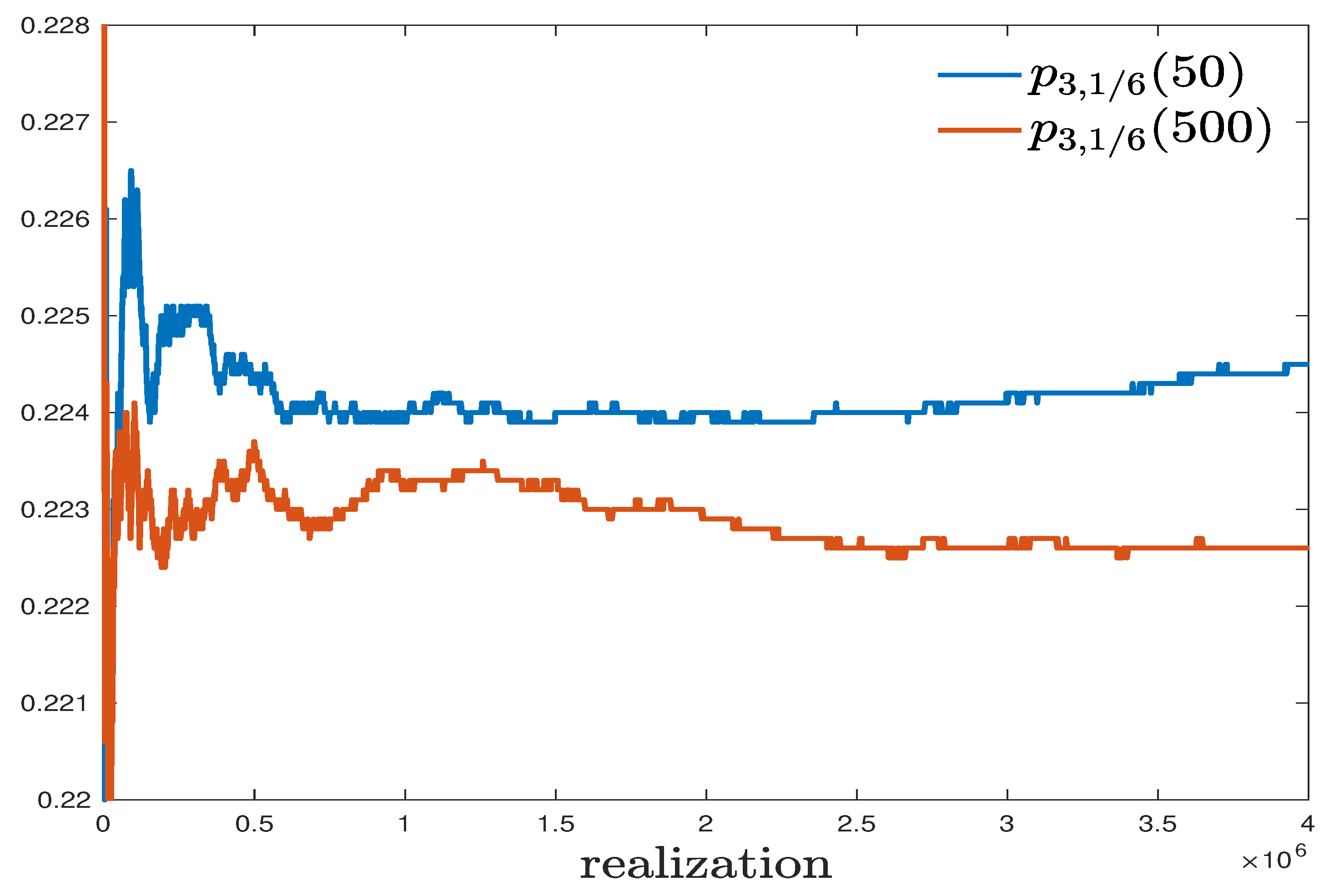
In addition to the aforementioned theoretical proof, the low-dimensional nonmonotonicity can also be verified in numerical simulation. In
Figure 2, we present numerical approximations of
and
achieved from
i.i.d. stochastic realizations.
In
Figure 2, a significant difference between the blue and red curves is observed. With
i.i.d. stochastic realizations, we have the frequencies
So, their standard deviations can be bounded from above by
. However, the difference between our approximations is about
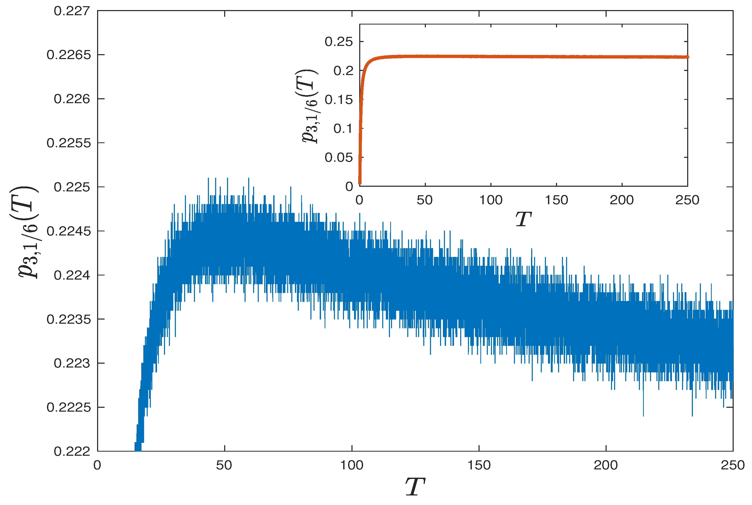
, which is larger than 4 times the upper bound of standard deviation. In
Figure 3, we numerically approximate the single edge density
for different
T with spacing
, and each point is evaluated by
i.i.d. stochastic realizations. In spite of some stochastic fluctuations, the trend of nonmonotonicity is clear and the probability seems to reach maximum at
.
4. Characterization of Phase Diagram
In this section, we focus on the (potential) phase diagram of edge percolation in FRI. We start with proving the uniqueness of infinite cluster in FRI by the classical “finite energy” argument. We put technical details of the proof in
Appendix B.
Theorem 2. For any and , Remark 6. Theorem 2 is similar to, though slightly stronger than, Theorem 4 [5], where the uniqueness was proved for sufficiently large T’s. Theorem 3. For all and FRI , we have the following:
If has an infinite cluster almost surely, then so does for all .
(Theorem 1, [5]) For all , there is a such that for all , almost surely percolates. Let be the critical edge density for dimensional Bernoulli bond percolation. For any , there exist some such that percolates almost surely for . Moreover, for any fixed d, as .
For any , there is , such that for all , percolates almost surely for all .
For any and , there exists constant such that
- (a)
when , , , almost surely percolates;
- (b)
when , , , almost surely percolates.
Remark 7. A statement equivalent to Claim (iii) Theorem 3 has also been proved in 5), Remark V.5.3, [10]. Proof. Note that by Theorem 2, one may focus only on the existence of infinite cluster.
Claim (i) is an immediate result of the monotonicity of
with respect to
u. For Claim (iii) and (iv), the key idea is to bound
from below by a supercritical Bernoulli percolation. Without loss of generality, one may first consider vertex 0, edge
, and the collection of fibers with length
that start from 0 and traverse
in their first jump. We denote the number of such paths by
. Recalling the definition of
, there are
fibers starting from 0. While for each of them, the probability it has length at least 1 is
, and the probability it takes
in the first step is
. Thus, by the thinning property of Poisson distribution, we have
Similarly, one can define
to be the number of fibers that start from
and traverse
in their first jump. By independent increment property of PPP,
is independent and identically distributed as
. Define the event as
Moreover, for any edge
, one can also define
in the exact same way. Thus,
form a i.i.d. sequence of
. Once again, define
Thus, the collection of good edges by definition forms a Bernoulli bond percolation with single edge density
which percolates when
Therefore, for any
, we take
, where
. Note that a good edge is by definition always traversed by the FRI. Claim (iii) is now a direct result of (
25), the fact that
reaches its maximum of
at
, and that
as
.
Now, for (iv), note that for a fixed
u, say
, by Theorem 1 [
5], there is a
such that for all
,
has an infinite cluster almost surely. With Claim (i), we now know this also holds for all
. In (iii), we showed that
. Thus, there is always a
such that
for all
. Thus, we have an infinite cluster almost surely for all
T from
all the way to infinity.
The proof of (v) is based on some more careful controls of exponents in constructing the infinite cluster in [
5]. As it is redundant to repeat the shared part of our construction in full details, we just point out modifications and estimates necessary to our proof here. Note that it is sufficient to prove for
.
To be specific, let
be any sufficiently small positive constant and
,
. By [
5], we know that it is sufficient to prove the following three events happen with sufficiently high probability (i.e., larger than
for some given
), corresponding to the conditions 1–3 introduced in Definition 3 of [
5]:
Assume that is the union of two independent FRI copies and (by the property of Poisson point processes). For any box , there exists a connected cluster in traversing and . We denote this event by E.
For any such that and two connected clusters and (containing x and y, respectively) in , if , , and , then and are connected by within . We denote this event by F.
There is no path starting from and intersecting . In addition, for , there is no path starting from and intersecting , and no path starting from and intersecting . We denote this event by G.
□
First, for event E, we need an estimate for the capacity of trajectories of several simple random walks.
Lemma 4 (Lemma 5, [
11]).
Let be a sequence of independent simple random walks on and . Then, By Lemma 4 and the same approach mentioned in the proof of Lemma 6 [
11], we can get a stronger version of Lemma 6 [
11]:
When
, note that the number of paths traversing
with length at least
T is a Poisson random variable with parameter
. By the large deviation bound for Poisson distribution, the probability of the event that there exists one path traversing
with length at least
T is larger than
. Take
in (
26), then, we have
When
, we do the same construction in Section 4.3 of [
5] by using the paths in
with length at least
T (note that we will use (
26) for
times but not only
times, where
). Similarly, by (
26) and large deviation bound for Poisson distribution, we have
Meanwhile, by Lemma 8 of [
11], we can ensure that the connected cluster mentioned above is contained by
with a probability of at least
for some
. In conclusion, for
,
and for
,
For
F, by Lemma 3.4 of [
12], we have that there exists constants
such that
Then, by (
31), Lemma 3.1 of [
6], and the approach in Lemma 12 of [
11], we have
For event
G, for any
, since
, we have
For the remaining subevents of
G, the estimates are similar. In conclusion,
Finally, by (
29), (
30), (
32), and (
34), it is elementary to check that when
is large enough, events
E,
F, and
G all happen with sufficiently high probability.
At the same time, we also have the following result on the subcritical phase when u is large. This, together with Claim (iv) of Theorem 3, characterize the asymptotic order of the phase diagram.
Proposition 2. For , there exists and such that for any and , does not have an infinite cluster almost surely.
Proof. This proposition is a direct corollary of the proof of Theorem 2 [
5]. By Section 7 of [
5], it has been proved that for any
,
does not have an infinite cluster a.s. if
satisfies the following two conditions:
For condition 2, it is sufficient to have
Note that
. In order to have
, we only need
In conclusion, if we take and , then condition 1, 2 hold for any and . □
5. Numerical Exploration on Phase Transition
The previous section provides (partial) characterizations on the super and subcritical phases of FRI, while it remains unknown whether there is a unique critical value
such that FRI almost surely percolates when
and has no infinite cluster when
. In this section, we make numerical explorations towards this direction. The general guidelines behind criteria of numerical tests in this section are mostly inspired by [
13,
14].
In order to investigate the existence and uniqueness of
, we develop the following parallel computing algorithm in order to efficiently sample the configuration within a large box in
of size
N, with data transferred within up to 80 cores via the Message Passing Interface (MPI). In Section 4.1 of [
5], it has been shown that we can sample the configuration of FRI restricted within an infinite set
K by Algorithm 1:
| Algorithm 1 Finitary Random Interlacement. |
Divide the vertices into mutually independent batches and distribute one batch to one processor. For s-th batch, for any , sample an independent random variable . Then, sample a sequence of i.i.d. random walks independent to , with distribution . For each trajectory of the random walk mentioned above, if escapes from K (i.e., for any , ), then start a new independent random walk with distribution and collect its trajectory ; if not, jump to the next trajectory . Collect all the trajectories from all processors.
|
Since
is identically distributed as the collections of all fibers in
which traverse
K, we have that
. Using the aforementioned algorithm, one can naturally look at the size (in either cardinality or diameter) of the largest connected component within a large box in
of size
N, say
. In the supercritical phase, there should be a macroscopic largest connected component within
, since it should, with high probability, be the largest cluster in the intersection(s) between the infinite cluster and our box. Meanwhile, in the subcritical phase, the largest connected component should be microscopic with respect to
N. See
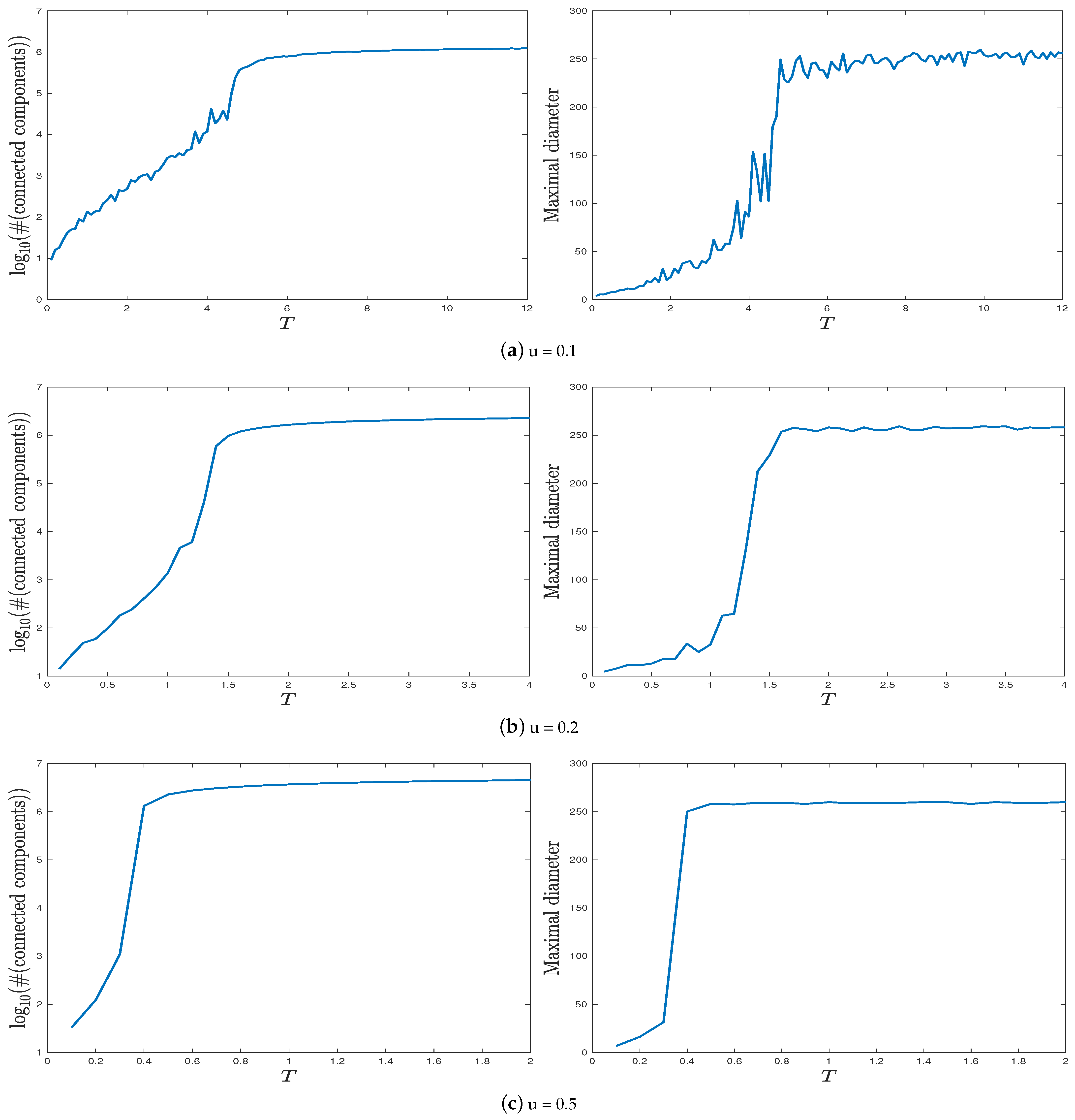
Figure 1a for illustration. In
Figure 4, we present stochastic simulation results on the cardinality and maximal diameter of the FRI’s largest connected components within
, for
,
, and various
T’s, under only one realization. In order to manifest the phase transition more clearly, we choose different ranges of
T under different
u. Although the curves are not smooth due to some random fluctuations and size effects, numerical evidences seem to strongly support the existence and uniqueness of
, which seems to be smaller as
u becomes larger.
Figure 4 strongly supports the existence of a unique critical fiber length, at least for the
u’s we chose. This encourages us to extend the test for all combinations of
’s within an appropriate grid
with
,
. Noting that the computational cost grows as
, we need to work on a smaller
. In order to avoid the extra randomness due to the smaller box size, we run 100 i.i.d. FRI copies for each combination of
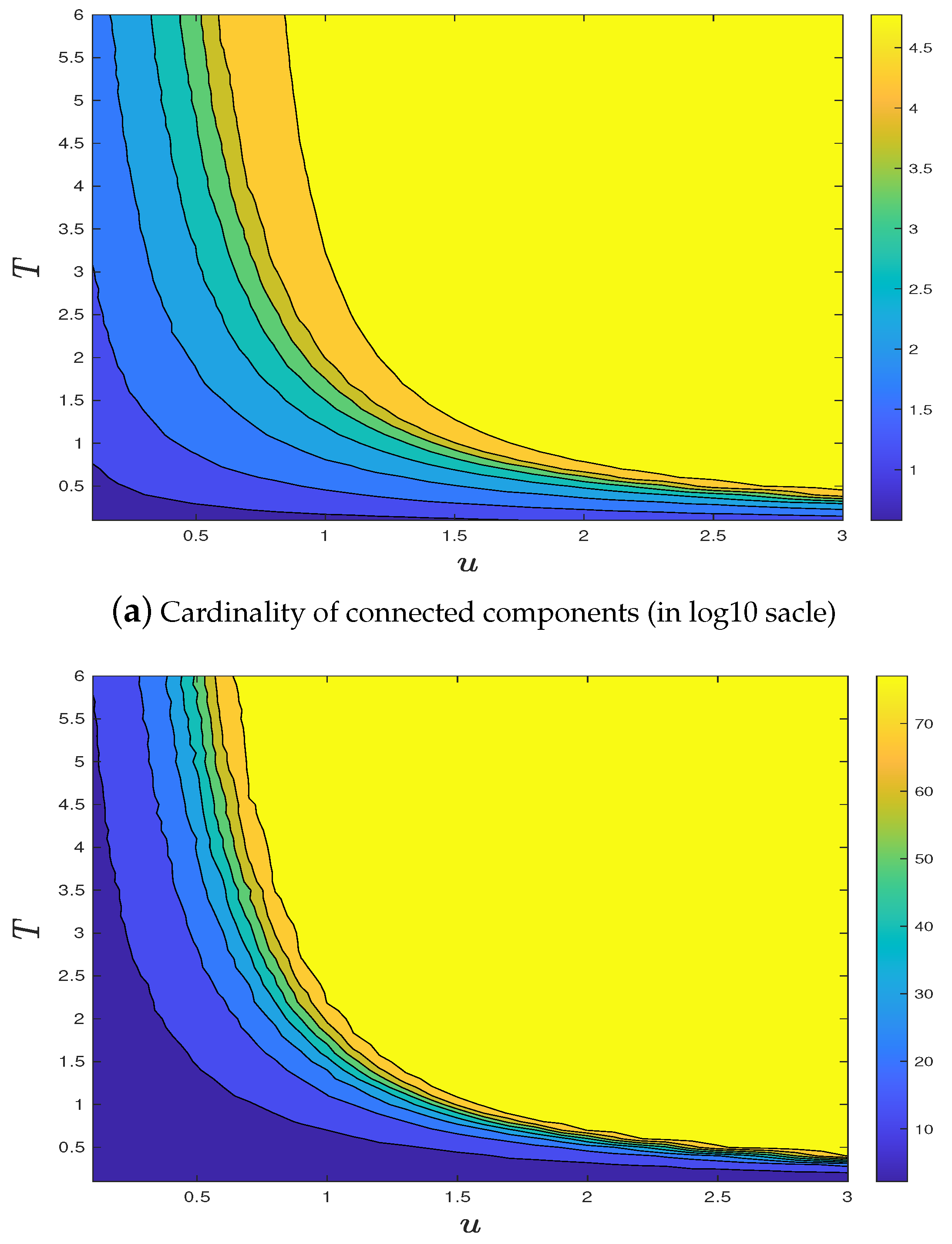
and approximate the expected size of the largest cluster. Results shown in
Figure 5 indicate that the existence and uniqueness of critical fiber length seem to hold for all
u’s.
Based on the aforementioned numerical evidences, we propose the following conjecture:
Conjecture 1. For alland, there is asuch that for
Remark 8. Part of Conjecture 1 is also briefly mentioned in a revised version of [5] without further study on (non)monotonicity or numerical evidences. If we for now accept the existence of critical value in the conjecture above, we then explore the shape and asymptotic of the curve of
. With the help of monotonicity over
u (Claim (i) Theorem 3), we use the following hill climbing algorithm (Algorithm 2) and record the ascending path
, with small spacing
,
,
,
. This algorithm significantly reduces the numerical costs in finding the boundary of phase transitions (as shown in
Figure 6).
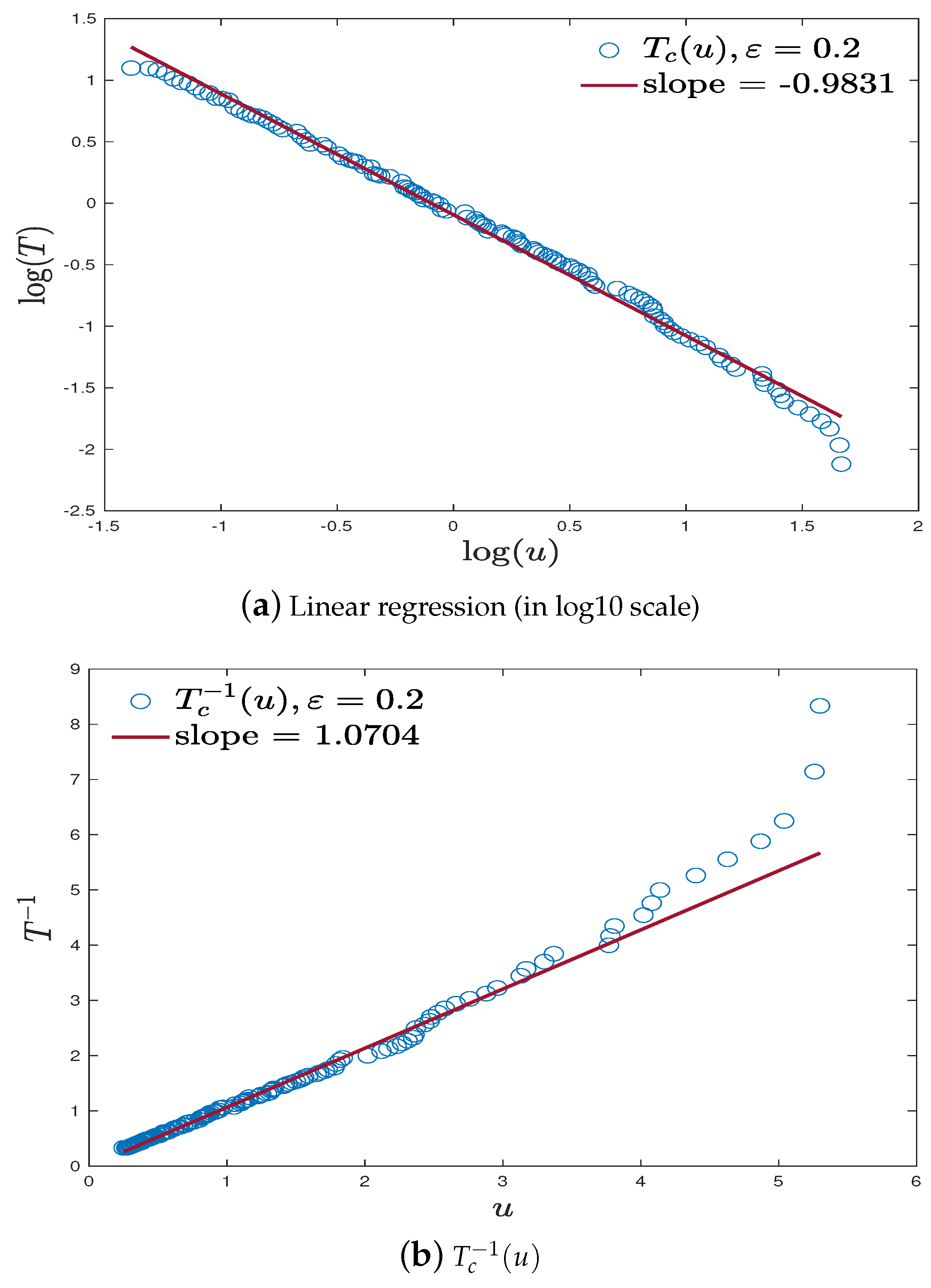
A linear regression on
(marked by circle), with
is shown in
Figure 7a. In addition, linear regression on
in
Figure 7b seems to indicate that the exponent in the upper bound of
in Claim (v) Theorem 3 is close to 1. This observation together with the theoretical findings in Theorem 3 and Proposition 2 motivates us to propose the following conjecture:
Conjecture 2. For all,
| Algorithm 2 Hill climbing algorithm. |
Input: The box size N, A sufficiently small initial , a sufficiently large initial , spacings and and a threshold . Start from and . Run one realization of FRI under the parameters and calculate the maximal diameter of the largest cluster of such FRI. If , , go to Step 5. If , and mark it by circle, go to Step 5. Terminate when , otherwise go back to Step 2 with parameters .
Output: The path |
Remark 9. It is worth noting that, as a result of the finite size effect of box size N, the estimated slope in linear regression under logarithm scale can be sensitive with respect to ϵ. We found in simulation that slope equals to when , when , when , when , and when . Recalling the theoretical upper bound of in Claim (iv) Theorem 3, and lower bound in Proposition 2, it is not hard to prove that slopes converge to , as for all . So, for , it seems the phase diagram has best precision when . Thus, we plot under this setting and find that the slope in linear regression is , which is very close to theoretical value 1. Here, we only use 112 points for linear regression and the remaining 9 points seem to deviate from the line. The possible reason is that is very small for large u and thus might not be precisely captured.


