Composite Multiscale Cross-Sample Entropy Analysis for Long-Term Structural Health Monitoring of Residential Buildings


Abstract
1. Introduction
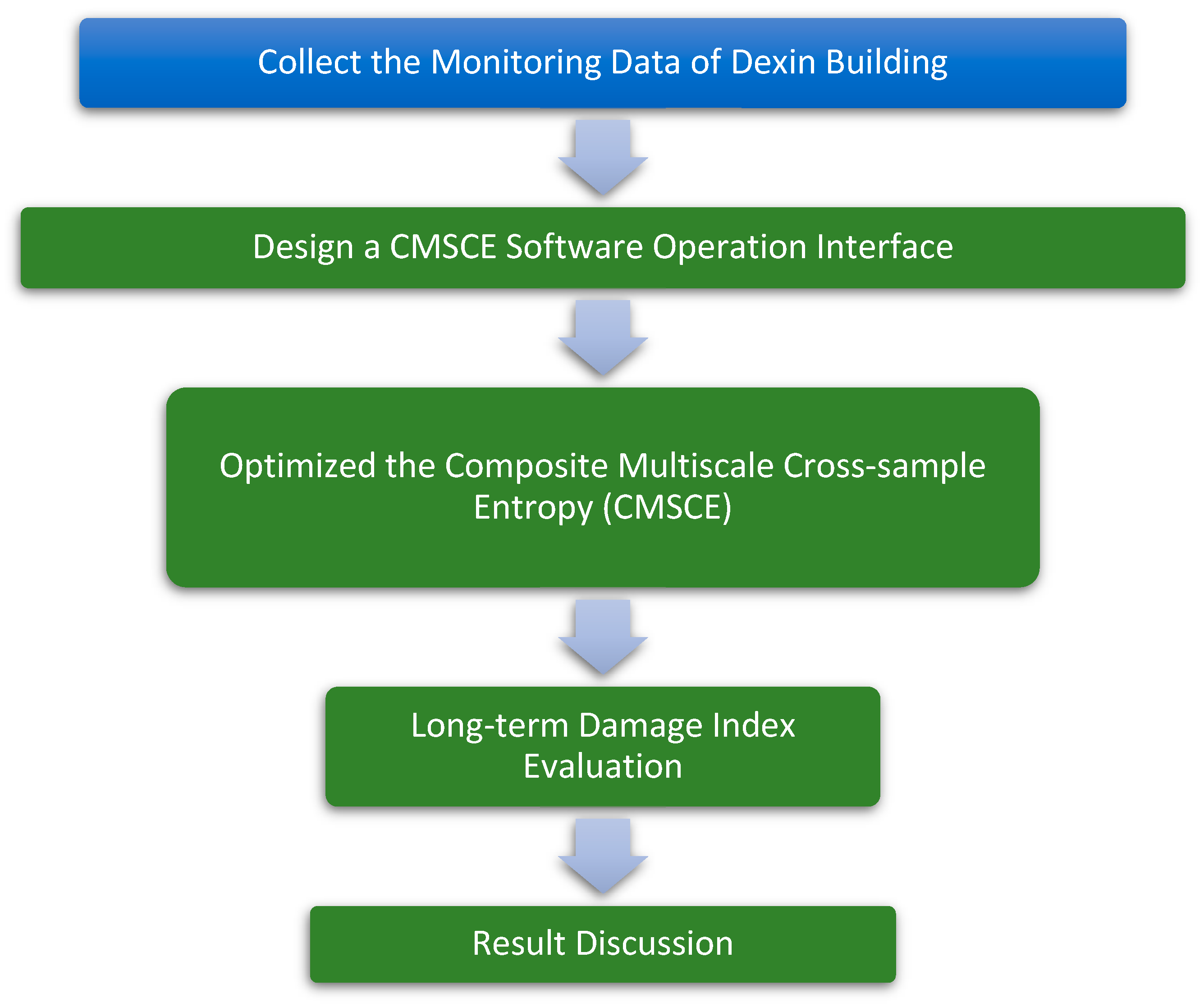
2. Methodology
2.1. Composite Multiscale Cross-Sample Entropy Method
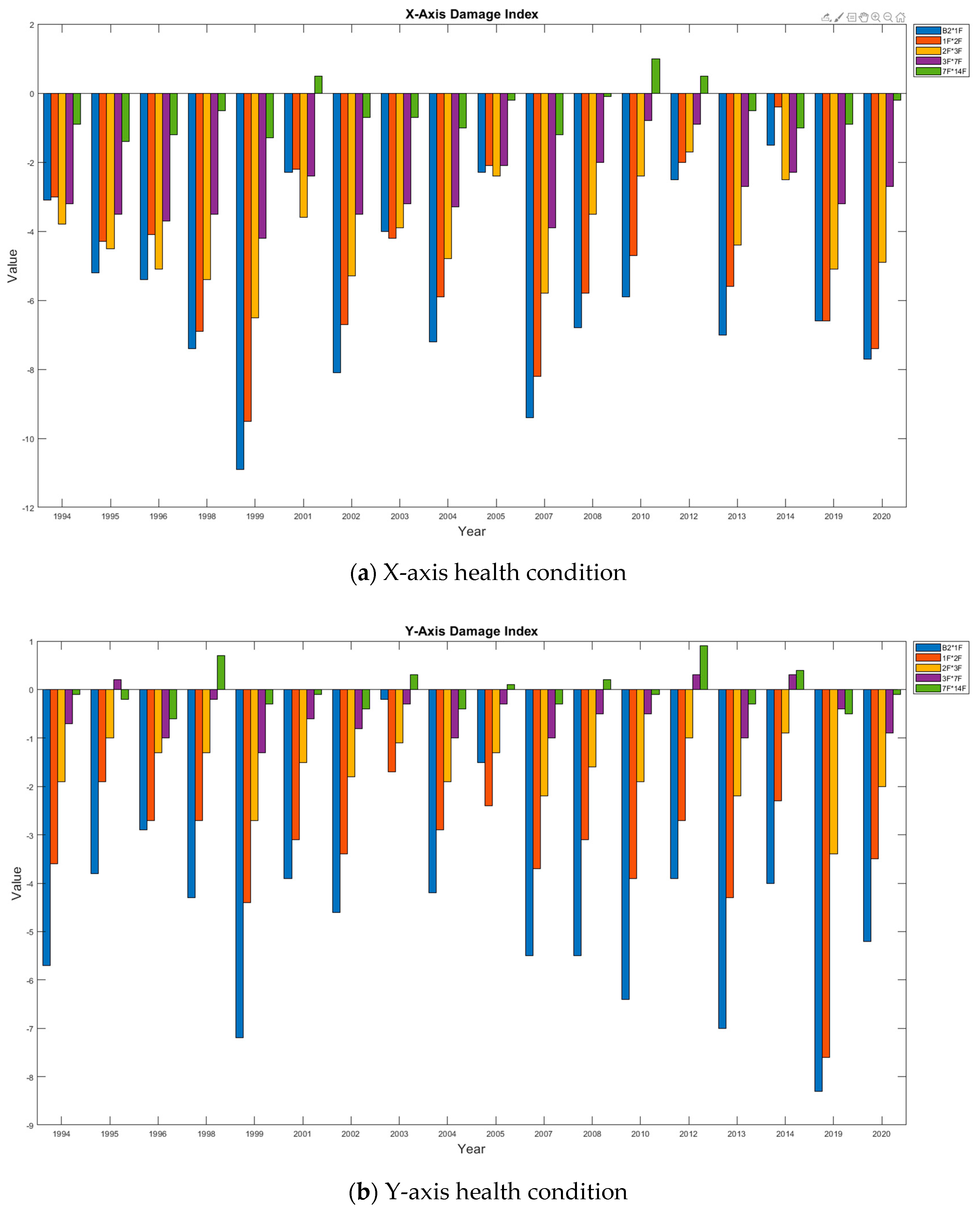
2.2. DI Measure
3. Long-Term Monitoring of Practical Residential Buildings
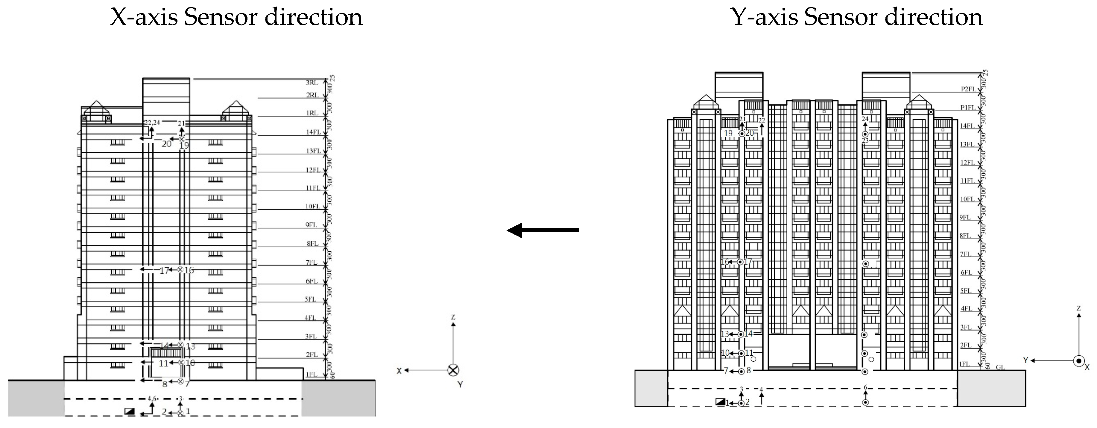
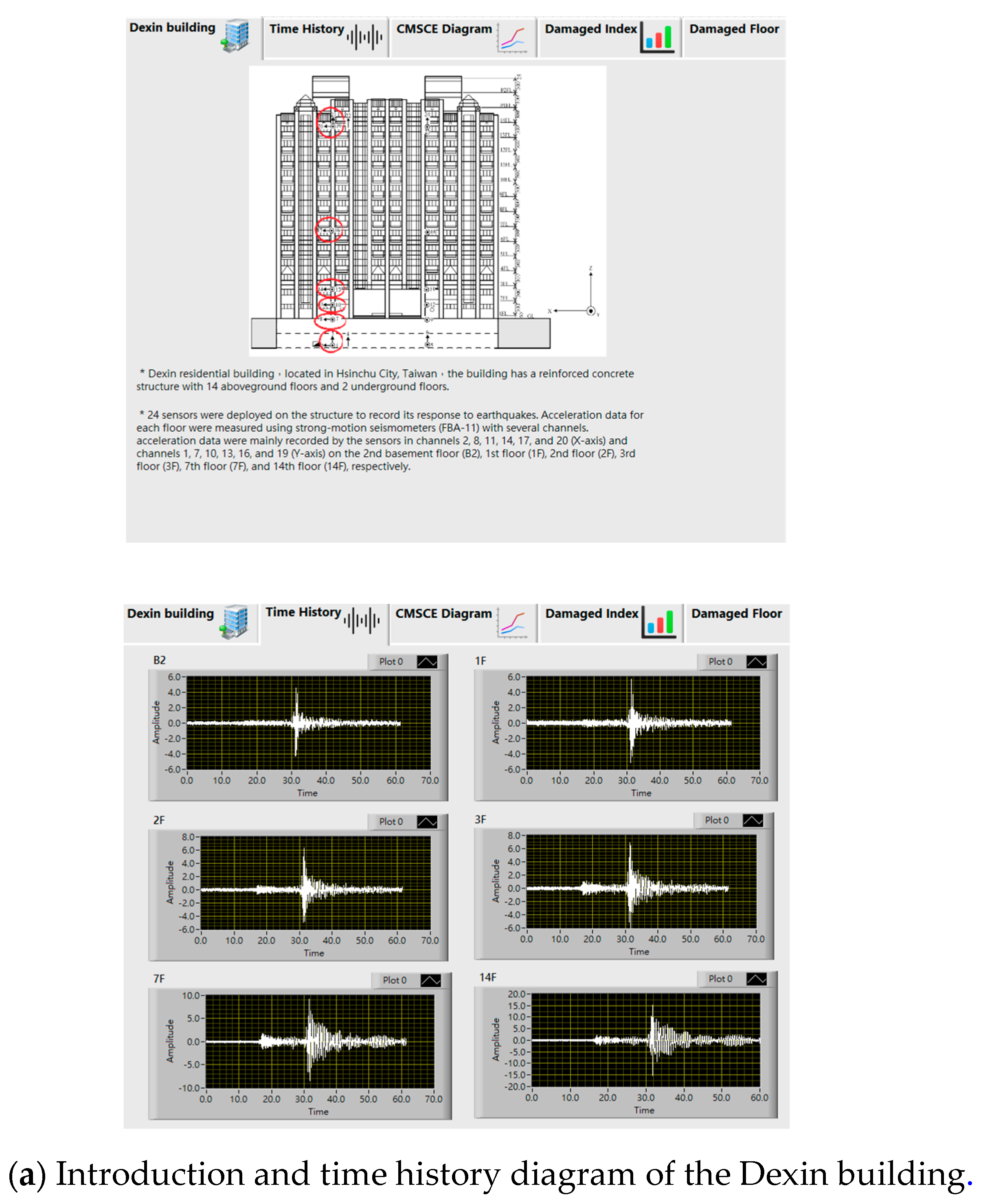
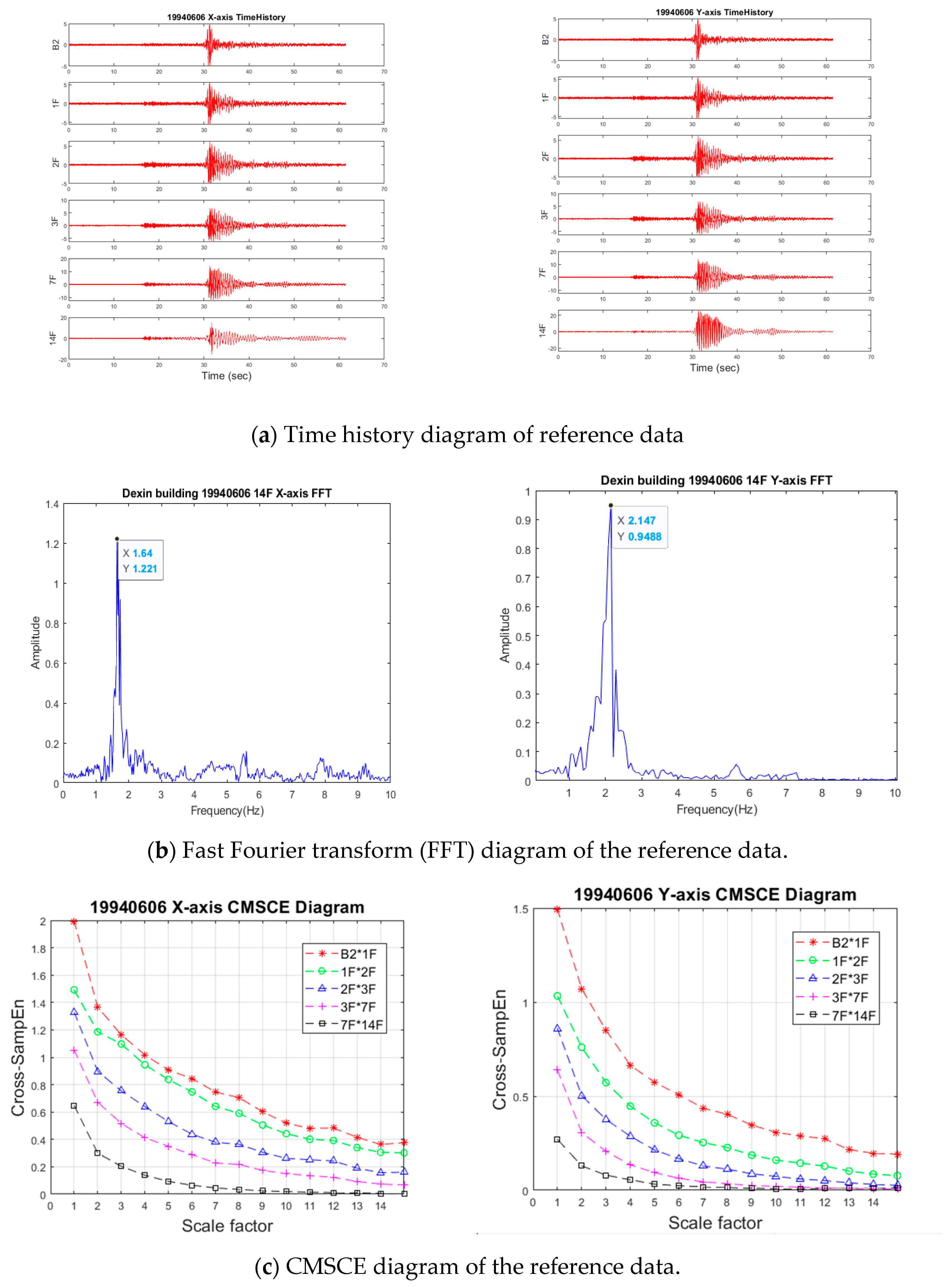
3.1. Introduction of the Dexin Residential Building
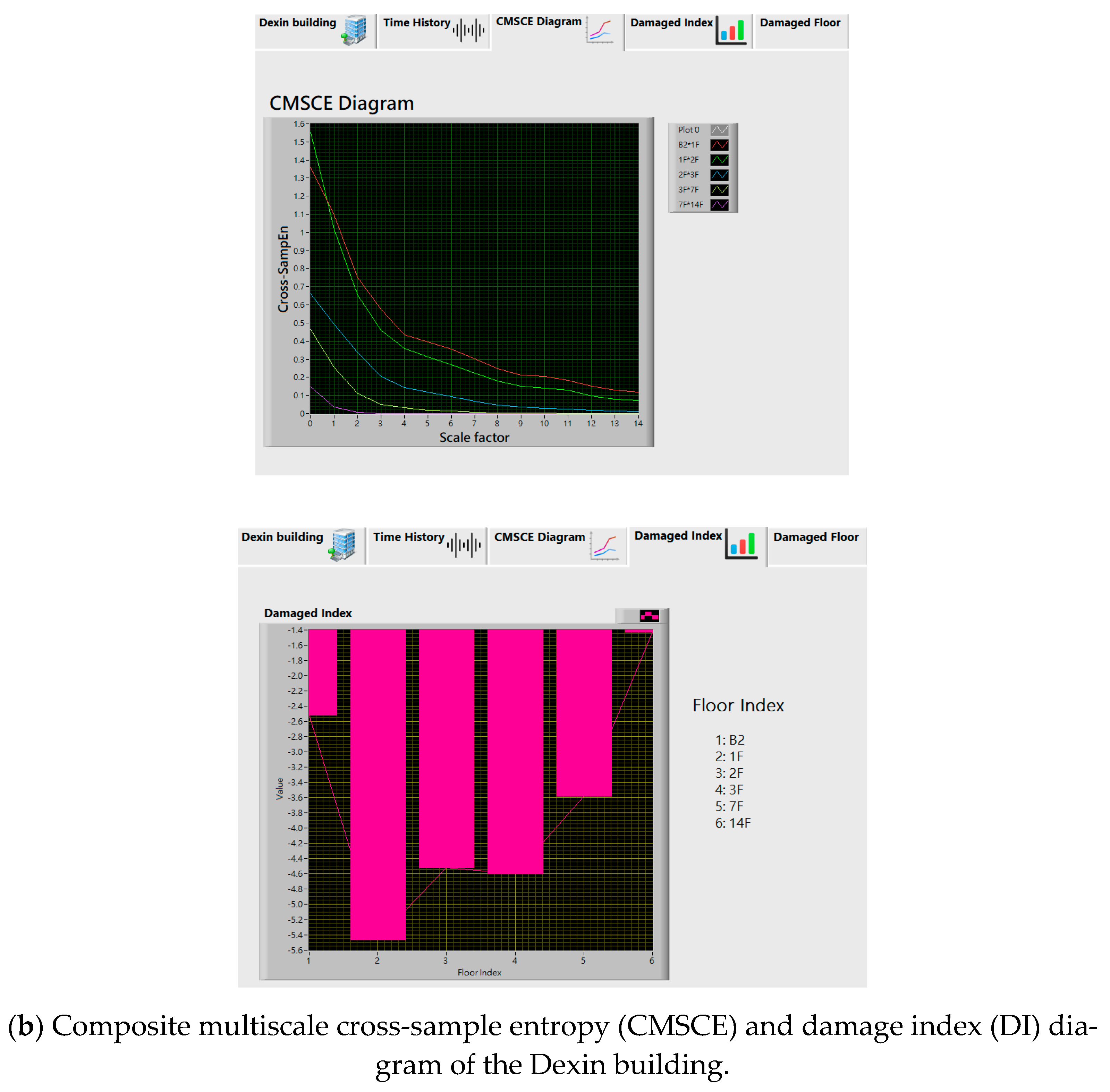
3.2. CMSCE Labview User Interface
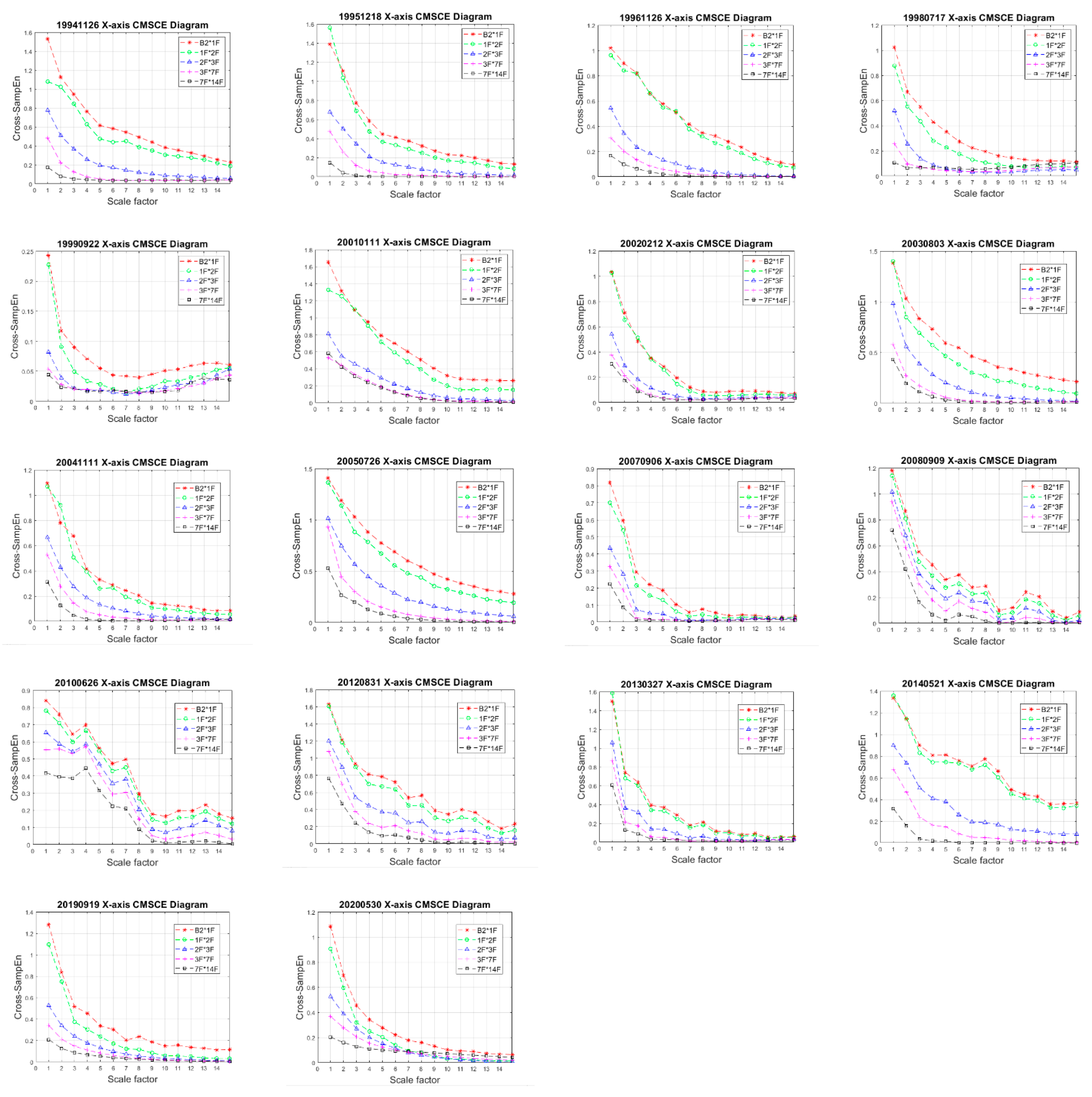
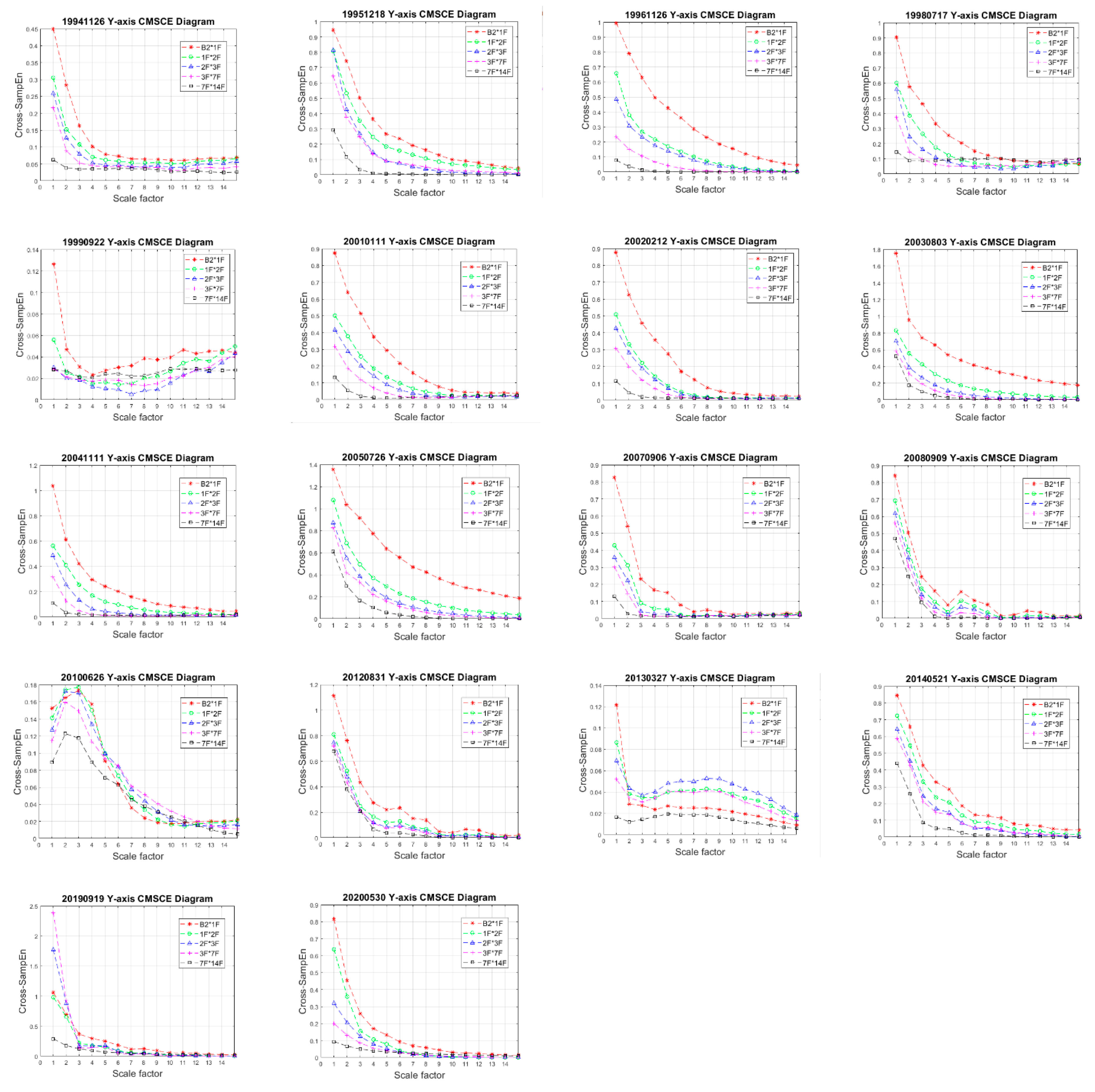
3.3. Evaluation of Long-Term Monitoring
3.3.1. CMSCE Diagram Analysis
3.3.2. DI Analysis
3.4. Earthquake Analysis
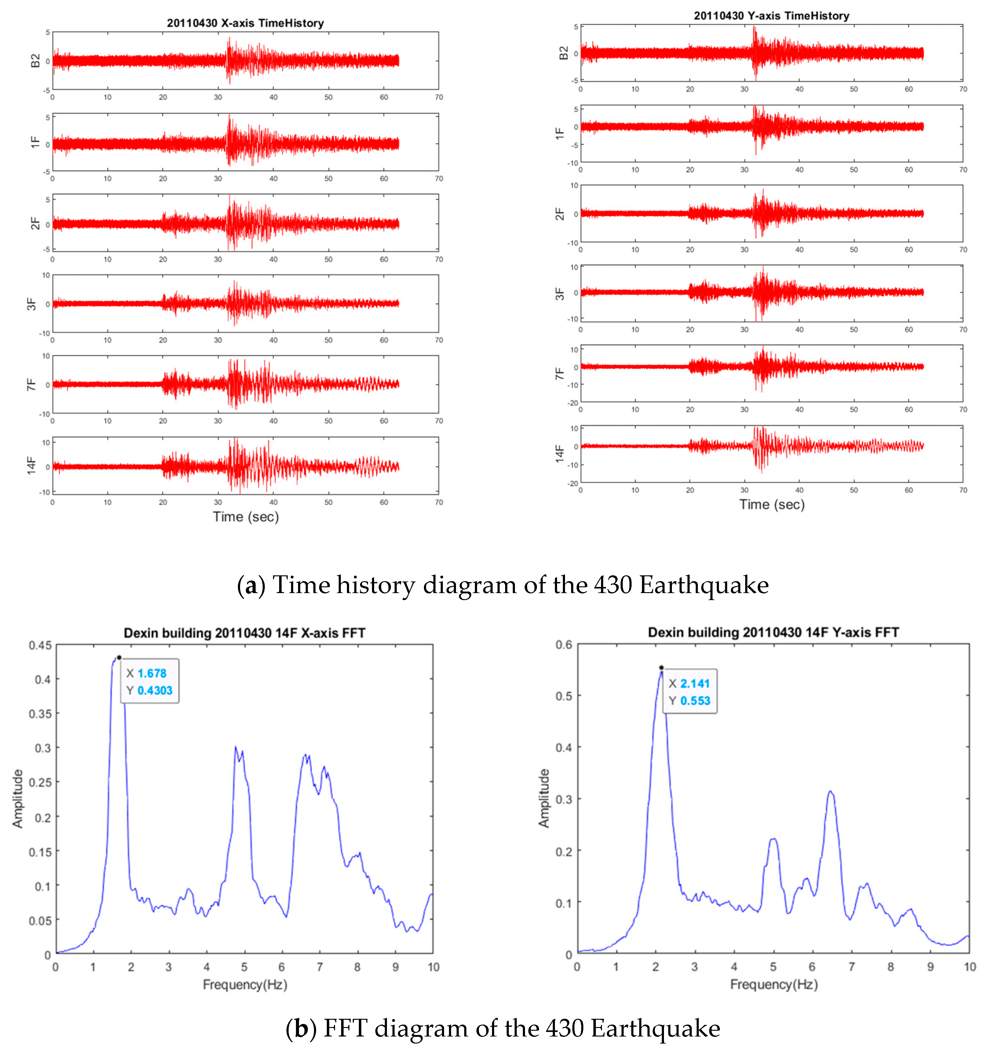
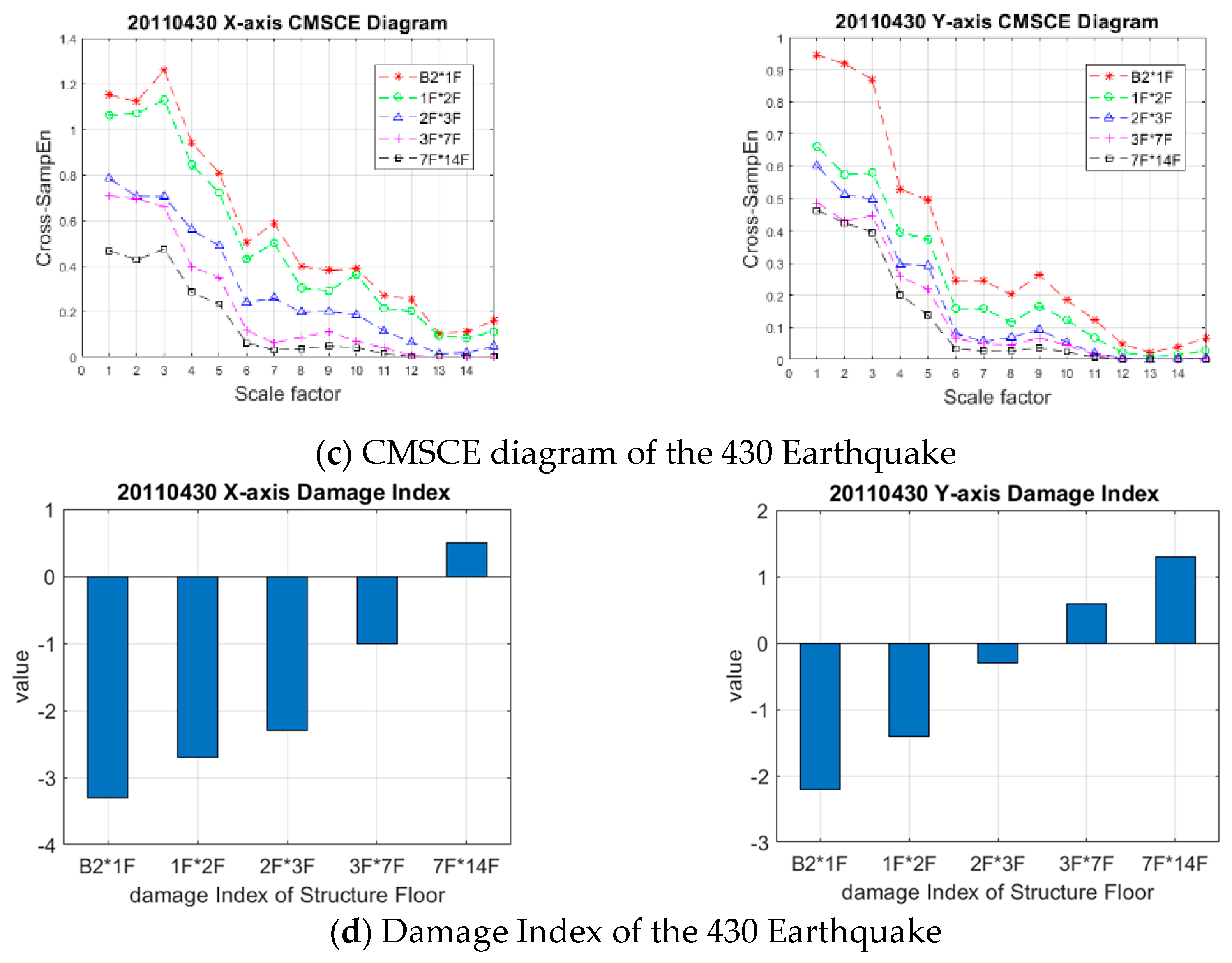
3.4.1. 430 Earthquake
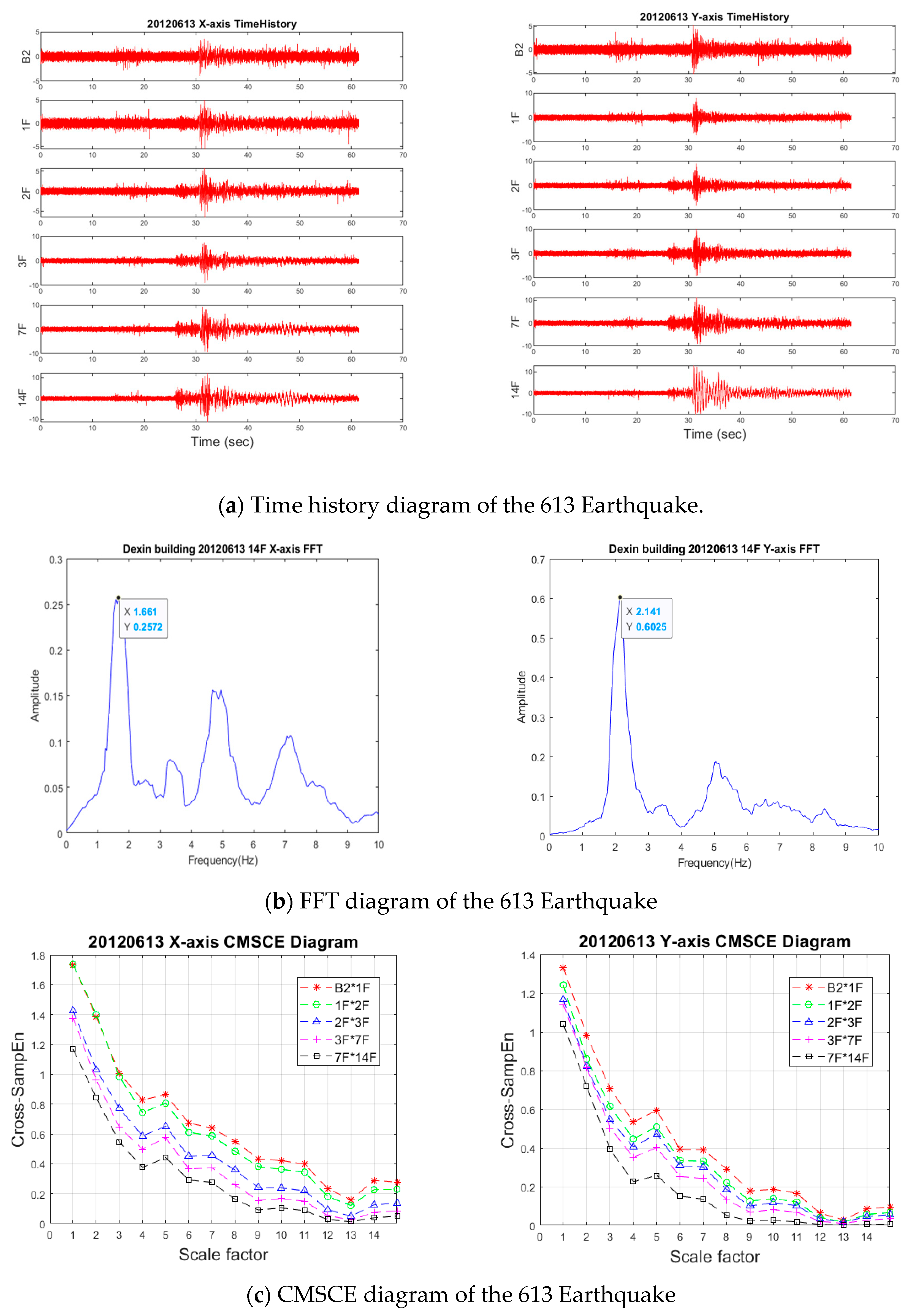
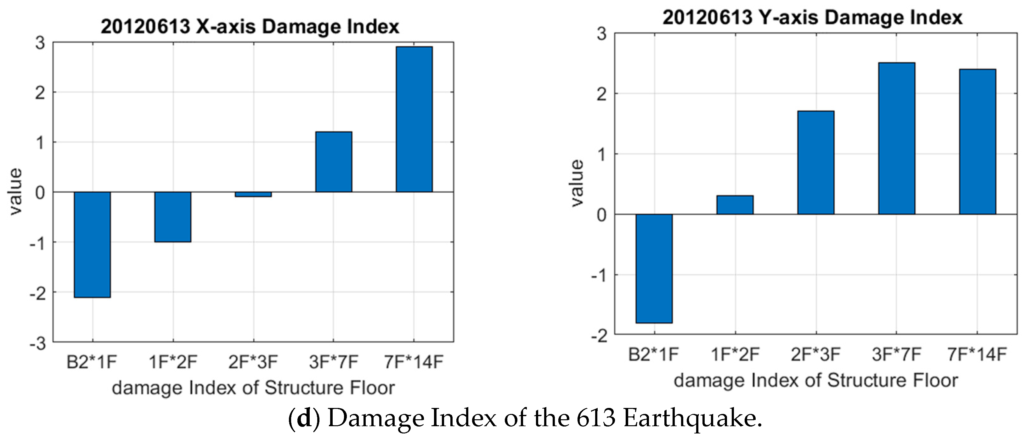
3.4.2. 613 Earthquake
4. Conclusions
Author Contributions
Funding
Conflicts of Interest
References
- Kim, H.; Bartkowicz, T. Damage detection and health monitiring of large space structure. In Proceedings of the Structures, Structural Dynamics, and Materials Conference, 34th and AIAA/ASME Adaptive Structures Forum, La Jolla, CA, USA, 19–22 April 1993; pp. 3527–3533. [Google Scholar]
- Zhang, H.; Schulz, M.J.; Naser, A.; Ferguson, F.; Pai, P.F. Structural health monitoring using transmittance functions. Mech. Syst. Signal Process. 1999, 13, 765–787. [Google Scholar] [CrossRef]
- Lee, J.M.; Kim, J.D.; Yun, C.B.; Yi, J.H.; Shim, J.M. Health-monitoring method for bridges under ordinary traffic loadings. J. Sound Vib. 2002, 257, 247–264. [Google Scholar] [CrossRef][Green Version]
- Chang, P.C.; Flatau, A.; Liu, S. Health monitoring of civil infrastructure. Struct. Health Monit. 2003, 2, 257–267. [Google Scholar] [CrossRef]
- Lin, T.-K.; Kiremidjian, A.; Lei, C.-Y. A bio-inspired structural health monitoring system based on ambient vibration. Smart Mater. Struct. 2010, 19, 115012. [Google Scholar] [CrossRef]
- Shokravi, H.; Shokravi, H.; Bakhary, N.; Rahimian Koloor, S.S.; Petrů, M. Health Monitoring of Civil Infrastructures by Subspace System Identification Method: An Overview. Appl. Sci. 2020, 10, 2786. [Google Scholar] [CrossRef]
- Clausius, R.; Walter, R. The Mechanical Theory of Heat-with its Applications to the Steam Engine and to Physical Properties of Bodies; John van Voorst: London, UK, 1865. [Google Scholar]
- Shannon, C.E. A Mathematical Theory of Communication. Bell Syst. Tech. J. 1948, 27, 379–423. [Google Scholar] [CrossRef]
- Pincus, S.M.; Gladstone, I.M.; Ehrenkranz, R.A. A regular statistic for medical data analysis. J. Clin. Monit. 1991, 7, 335–345. [Google Scholar] [CrossRef]
- Richman, J.S.; Moorman, J.R. Physiological time series analysis using approximate entropy and sample entropy. Am. J. Physiol. Heart Circ. Physiol. 2000, 278, H2039–H2049. [Google Scholar] [CrossRef]
- Lake, D.; Richman, J.S.; Griffin, M.P.; Moorman, J.R. Sample entropy analysis of neonatal heart rate variability. Am. J. Physiol. Regul. Integr. Comp. Physiol. 2002, 283, 789–797. [Google Scholar] [CrossRef]
- Costa, M.; Goldberger, A.L.; Peng, C.K. Multi scale entropy analysis of complex physiologic time series. Phys. Rev. Lett. 2002, 89, 068102. [Google Scholar] [CrossRef]
- Costa, M.; Goldberger, A.L.; Peng, C.K. Multi scale entropy analysis of biological signals. Phys. Rev. E 2005, 71, 021906. [Google Scholar] [CrossRef] [PubMed]
- Pincus, S.M.; Singer, B.H. Randomness and degrees of irregularity. Proc. Natl. Acad. Sci. USA 1996, 93, 2083–2088. [Google Scholar] [CrossRef] [PubMed]
- Fabrisa, C.; de Colleb, W.; Sparacinoa, G. Voice disorders assessed by (cross-) Sample Entropy of electroglottogram and microphone signals. Biomed. Signal Process. Control 2013, 8, 920–926. [Google Scholar] [CrossRef]
- Wu, S.D.; Wu, C.W.; Lin, S.G.; Wang, C.C.; Lee, K.Y. Time series analysis using composite multiscale entropy. Entropy 2013, 15, 1069–1084. [Google Scholar] [CrossRef]
- Yin, Y.; Shang, P.G.; Feng, G.C. Modified multiscale cross-entropy for complex time series. Appl. Math. Comput. 2016, 289, 98–110. [Google Scholar] [CrossRef]
- Wimarshana, B.; Wu, N.; Wu, C. Crack identification with parametric optimization of entropy & wavelet transformation. Struct. Monit. Maint. Int. J. 2017, 4, 33–52. [Google Scholar]
- Guan, X.F.; Wang, Y.X.; He, J.J. A Probabilistic Damage Identification Method for Shear Structure Components Based on Cross--Entropy Optimizations. Entropy 2017, 19, 27. [Google Scholar] [CrossRef]
- Lin, Y.H.; Huang, H.C.; Chang, Y.C.; Lin, C.; Lo, M.T.; Liu, L.Y.; Tasi, P.R.; Chen, Y.S.; Ko, W.J.; Ho, Y.L.; et al. Multi-scale symbolic entropy analysis provides prognostic prediction in patients receiving extracorporeal life support. Crit. Care 2014, 18, 548. [Google Scholar] [CrossRef]
- Lin, Y.H.; Lin, C.; Ho, Y.H.; Wu, V.C.; Lo, M.T.; Hung, K.T.; Liu, L.Y.; Lin, L.Y.; Huang, J.W.; Peng, C.K. Heart rhythm complexity impairment in patients undergoing peritoneal dialysis. Sci. Rep. 2016, 6, 280202. [Google Scholar] [CrossRef]
- Chiu, H.C.; Ma, H.P.; Lin, C.; Lo, M.T.; Lin, L.Y.; Wu, C.K.; Chiang, J.Y.; Lee, J.K.; Hung, C.S.; Wang, T.D.; et al. Serial heart rhythm complexity changes in patients with anterior wall ST segment elevation myocardial infarction. Sci. Rep. 2017, 7, 43507. [Google Scholar] [CrossRef]
- Lin, T.K.; Liang, J.C. Application of multi scale (cross-) sample entropy for structural health monitoring. Smart Mater. Struct. 2015, 24, 085003. [Google Scholar] [CrossRef]
- Lin, T.K.; Tseng, T.C.; Lainez, A.G. Three dimensional structural health monitoring based on multiscale cross sample entropy. Earthq. Struct. 2017, 12, 673–687. [Google Scholar]
- Lin, T.K.; Lainez, A.G. Entropy Based Structural Health Monitoring System for Damage Detection in Multi Bay Three Dimensional Structures. Entropy 2018, 20, 49. [Google Scholar]


| Channel | Axis | Location |
|---|---|---|
| CH01 | ) | |
| CH02 | ) | |
| CH03 | ||
| CH04 | ||
| CH05 | ||
| CH06 | ||
| CH07 | ||
| CH08 | ||
| CH09 | ||
| CH10 | ||
| CH11 | ||
| CH12 | Y | |
| CH13 | Y | |
| CH14 | X | |
| CH15 | Y | |
| CH16 | Y | |
| CH17 | X | |
| CH18 | Y | |
| CH19 | Y | |
| CH20 | X | |
| CH21 | Z | |
| CH22 | Z | |
| CH23 | Y | |
| CH24 | Z |
Publisher’s Note: MDPI stays neutral with regard to jurisdictional claims in published maps and institutional affiliations. |
© 2020 by the authors. Licensee MDPI, Basel, Switzerland. This article is an open access article distributed under the terms and conditions of the Creative Commons Attribution (CC BY) license (http://creativecommons.org/licenses/by/4.0/).
Share and Cite
Lin, T.-K.; Lee, D.-Y. Composite Multiscale Cross-Sample Entropy Analysis for Long-Term Structural Health Monitoring of Residential Buildings. Entropy 2021, 23, 60. https://doi.org/10.3390/e23010060
Lin T-K, Lee D-Y. Composite Multiscale Cross-Sample Entropy Analysis for Long-Term Structural Health Monitoring of Residential Buildings. Entropy. 2021; 23(1):60. https://doi.org/10.3390/e23010060
Chicago/Turabian StyleLin, Tzu-Kang, and Dong-You Lee. 2021. "Composite Multiscale Cross-Sample Entropy Analysis for Long-Term Structural Health Monitoring of Residential Buildings" Entropy 23, no. 1: 60. https://doi.org/10.3390/e23010060
APA StyleLin, T.-K., & Lee, D.-Y. (2021). Composite Multiscale Cross-Sample Entropy Analysis for Long-Term Structural Health Monitoring of Residential Buildings. Entropy, 23(1), 60. https://doi.org/10.3390/e23010060