Given the assumptions above,
, implying that the likelihood is
where
denotes the set of observed values of vectors
for
. As in
Section 3, we will consider an improper prior for
, given by
and our reference density,
, will be proportional to a constant, leading to a surprise function equivalent to the (full) posterior distribution. These choices correspond to steps 1 and 2 of
Table 1. These modeling choices imply the following posterior density:
where
and
.
To implement Step 3 of
Table 1, we need to find the maximum a posteriori of (
17) under the constraint
, i.e., we need to maximize the posterior in
. Since we are testing the rank of matrix
, as discussed in the beginning of
Section 4, it is necessary to maximize the posterior assuming the rank of
is
r,
. Thanks to the modeling choices made here—Gaussian likelihood and Equation (
16) as prior—our posterior is almost identical to a Gaussian likelihood, allowing us to find this maximum using a strategy similar to that proposed by [
2], who derived the maximum of the (Gaussian) likelihood function assuming a reduced rank for
. We will summarize Johansen’s algorithm, providing in
Appendix C a heuristic argument of why it indeed provides the maximum value of the posterior under the assumed hypotheses.
The second stage of Johansen’s algorithm requires the computation of the following sample covariance matrices of the OLS residuals obtained above:
and, from these, we find the
n eigenvalues of matrix
ordering them decreasingly
. The maximum value attained by the log posterior subject to the constraint that there are
r (
) cointegration relationships is
where
K is a constant that depends only on
T,
n and
by means of the marginal distribution of the data set,
. Since
represents the maximum of the log-posterior, to obtain
, one should take
, completing step 3 of
Table 1.
As in
Section 3, we compute
in step 4 by means of a Monte Carlo algorithm. It is easy to factor the full posterior (
17) as a product of a (matrix) normal and an Inverse-Wishart, suggesting a Gibbs sampler to generate random samples from the full posterior. See
Appendix B for more on the Inverse-Wishart distribution. Thus, the conditional posteriors for
and
are, respectively,
where
,
denotes the Inverse-Wishart,
is the number of lines of
, and
its OLS estimator, as above. From a Gibbs sampler set with these conditionals, we obtain a random sample from the full posterior to estimate
as the proportion of sampled vectors that generate a value for the posterior greater than
. Finally, we obtain
in the final step (5). The whole implementation for cointegration tests, following the assumptions made in this section, is summarized in
Table 4. See
Appendix A for more information on the computational resources needed to implement the steps given by
Table 4.
Results
Now we present, by means of four examples, the application of FBST as a cointegration test. In all the examples, we have adopted a Gaussian likelihood and the improper prior (
16). The Gibbs sampler was implemented as described above, providing 51,000 random vectors from the posterior (
17). The first 1000 samples were discarded as a burn-in sample, the remaining 50,000 being used to estimate the integral (
2). The tables show the e-value computed from the FBST and the maximum eigenvalue test statistics with their respective
p-values.
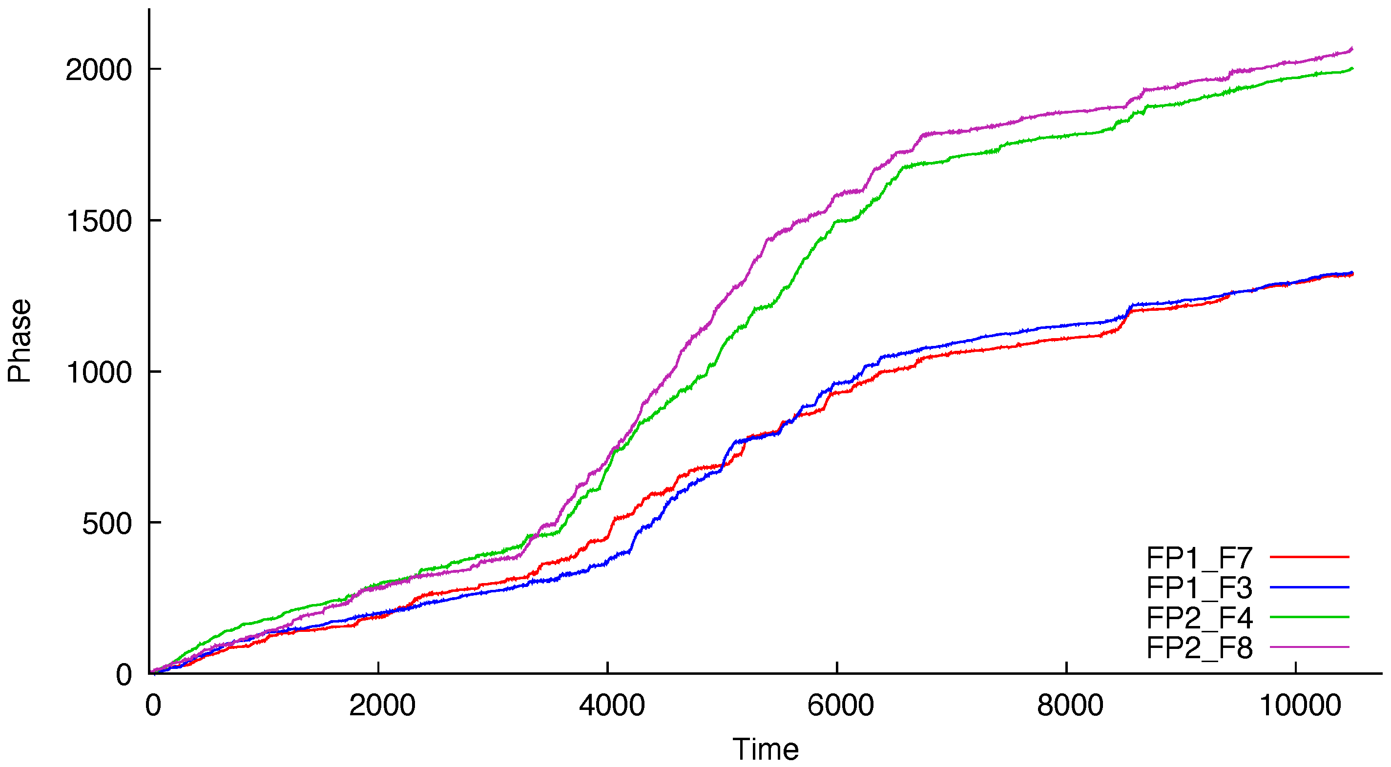
Example 1. We analyzed four electroencephalography (EEG) signals from a subject that has previously presented epileptic seizures. The original study, [44], had the aim of detecting seizures based on multiple hours of recordings for each individual and the cointegration analysis of the mentioned signals was presented by [45]. In fact, the cointegration hypothesis is tested using the phase processes estimated from the original signals. This is done by passing the signal into the Hilbert transform and then “unwrapping” the resulting transform. Sections 2 and 5 of [45,46] provide more details on the Hilbert transform and unwrapping. The labels of the modeled series refer to the electrodes on the scalp. As seen in
Figure 1 and
Figure 2, the series are called FP1-F7, FP1-F3, FP2-F4, and FP2-F8, where FP refers to the frontal lobes and F refers to a row of electrodes placed behind these. Even numbered electrodes are on the right side and odd numbered electrodes are on the left side. The electrodes for these four signals mirror each other on the left and right sides of the scalp. The recordings of the studied subject, an 11-year-old female, identified a seizure in the interval (measured in seconds)
. Therefore, like [
45], we analyze the period of 41 seconds prior to the seizure—interval
—and the subsequent 41 seconds—interval
—the seizure period. In the sequel, we will refer to these as
prior to seizure and
during seizure, respectively. Since the sample frequency has 256 measurements per second, there are a total of 10,496 measurements for each of the four signals. Ref. [
45] used 40 seconds for each period, obtaining slightly different results.
Figure 1 and
Figure 2 display the estimated phases based on the original signals. The model proposed by [
45] is a VAR(1), resulting in a VECM given by
Table 5 and
Table 6 present the results that essentially lead to the same conclusions obtained by [
45], even though they have based their findings on the trace test. See Table 8 of [
45].
The comparison between p-values and the FBST e-values must be made carefully, the main reason being the fact that p-values are not measures supporting the null hypothesis, while e-values provide exactly such a kind of support. That being said, a possible way to compare them is by checking the decision their use recommend regarding the hypothesis being tested, i.e., to reject or not the null hypothesis.
Frequentist tests often adopt a significance level approach: given an observed
p-value, the hypothesis is rejected if the
p-value is smaller or equal to the mentioned level, usually 0.1, 0.05, or 0.01. Since the cointegration ranks generate nested likelihoods, the hypotheses are tested sequentially, starting with null rank,
. For
Table 5, adopting a 0.01 significance level, the maximum eigenvalue test would reject
and
, and would not reject
. The same conclusions follow for
Table 6. Thus, the recommended action is to work, for estimation purposes for instance, assuming two cointegration relationships.
The question on which threshold value to adopt for the FBST was already mentioned on
Section 1.1, but it is worthwhile to underline it once more. We highly recommend a principled approach deriving the cut-off value from a loss function, which is specific for the problem at hand and the purposes of the analysis. A naive but simpler approach would be to reject the hypothesis if the e-value is smaller than 0.05 or 0.01, emulating the frequentist strategy. Even not recommending this path, since
p-values are not supporting measures for the hypothesis being tested while e-values are, the researcher may numerically compare
p-values and e-values in a specific scenario. If the researcher derived the
p-values from a generalized likelihood ratio test, it is possible to asymptotically compare them. The relationship is:
, where
m is the dimension of the full parameter space,
h the dimension of the parameter space under the null hypothesis,
the chi-square distribution function with
m degrees of freedom and
p the corresponding
p-value. See [
9,
12] for the proof of the asymptotic relationship between e-values and
p-values.
Since the maximum eigenvalue test is derived as a likelihood ratio test, this comparison may be done for the results of all the examples presented here, and more appropriately to this example, given its sample size of 10,496 observations. Regarding
Table 5 and
Table 6, one could be in doubt regarding whether to reject or not the hypothesis
since the e-values are larger than 0.01. However, for this model and hypothesis, the e-value corresponding to 0.01 is 0.436. Therefore, in both tables, one could reject the hypothesis and proceed to the next rank that has plenty of evidence in its favor. In conclusion, the practical decisions of both tests (FBST and maximum eigenvalue) would be the same: to not reject
.
Example 2 ([
47])
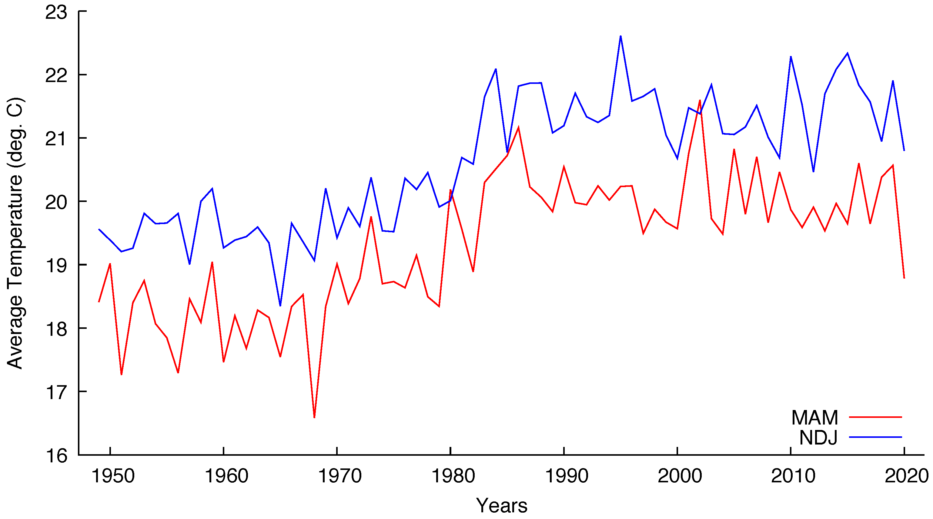
. Compare three methods for modeling empirical seasonal temperature forecasts over South America. One of these methods is based on a (possible) long-term cointegration relationship between the temperatures of the quarter March–April–May (MAM) of each year and the temperature of the previous months of November–December–January (NDJ). When there is such a relationship, the authors used the NDJ temperatures (of the previous year) as a predictor for the following MAM season. The original data set has monthly temperatures for each coordinate (latitude and longitude) of the covered area. The mentioned series of temperatures (MAM and NDJ) are computed as seasonal averages from this monthly data set by averaging over consecutive three months. Since we have data available from January 1949 to May 2020, the time series of monthly and seasonal average surface temperatures of length 72 for each grid point.
The authors of [
47] consider
as a two-dimensional vector, its first component being the seasonal (average) MAM temperature of year
t and the second component the seasonal NDJ temperature of the
previous year. They consider a VAR(2) without deterministic terms to model the series, resulting in a VECM
We have chosen five grid points corresponding to major Brazilian cities to test the cointegration hypothesis of the mentioned seasonal series. The coordinates chosen were the closest ones from: 23.5505
S, 46.6333
W for São Paulo; 22.9068
S, 43.1729
W for Rio de Janeiro; 19.9167
S, 43.9345
W for Belo Horizonte; 15.8267
S, 47.9218
W for Brasília and 12.9777
S, 38.5016
W for Salvador.
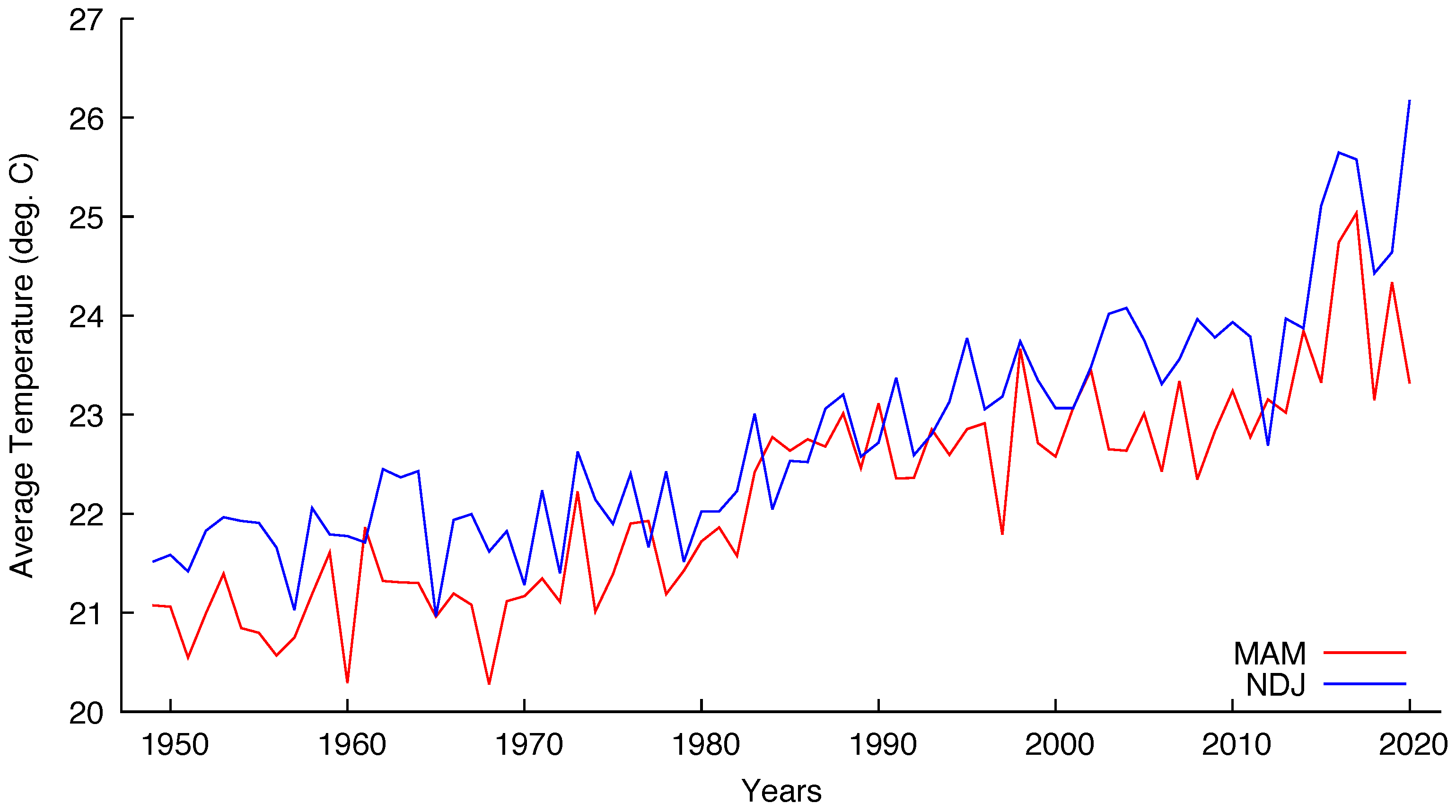
Figure 3 and
Figure 4 show the seasonal temperatures for São Paulo and Brasília, respectively, indicating that the cointegration hypothesis is plausible for both cities.
The results are shown in
Table 7. Assuming a significance level of 0.01, the maximum eigenvalue test reject the null rank and do not reject
for all the five cities. If we adopt the asymptotic relationship between
p-values and e-values for the model under analysis, we obtain an e-value of 0.276 corresponding to a 0.01
p-value for
. Therefore, the FBST would also reject the null rank for all the cities. The hypothesis
is not rejected since all the e-values are close to 1, once more agreeing with the maximum eigenvalue test.
One remark about Brasília seems in order. The city was built to be the federal capital, being officially inaugurated on 21 April 1960. The construction began circa 1957 and before that the site had no human occupation. The process of moving all the administration from Rio de Janeiro, the former capital, was slow and only the 1980 census detected a population over 1 million inhabitants. The present population is almost 3.2 million inhabitants living in the Federal District that includes Brasília and minor surrounding cities.
Figure 4 indicates that the seasonal temperatures began to rise exactly after 1980.
Example 3. we applied the FBST to the Finish data set used in their seminal work [2]. The authors used the logarithms of the series of
monetary aggregate, inflation rate, real income, and the primary interest rate set by the Bank of Finland to model the money demand, which, in theory, follows a long-term relationship. The sample has 106 quarterly observations of the mentioned variables, starting at the second trimester of 1958 and finishing in the third trimester of 1984. The chosen model was a VAR(2) with unrestricted constant, meaning that the series in
have one unit root with drift vector
and the cointegrating relations may have a non-zero mean. For more information about how to specify deterministic terms in a VAR see [
48], chapter 6. Seasonal dummies for the first three quarters of the year were also considered in the model chosen by [
2]. Writing the model in the error correction form, we have:
where
,
,
is a vector with constants and
denote the seasonal dummies for trimester
. The results are displayed in
Table 8.
In [
2], the authors concluded that there is, at least, two cointegration vectors, a conclusion that follows if one adopts a 0.01 significance level, for instance. Using the asymptotic relationship between
p-values and e-values for Equation (
26), we obtain, for
, an e-value of 0.998, and, for
, an e-value of 0.999, corresponding to a 0.01
p-value. These apparently discrepant values for the e-values are due to the high dimensions of the unrestricted (
) and under
(
for
and
for
) parameter spaces. Therefore, under this criterion, the FBST also rejects the null rank and
(since 0.132 < 0.998 and 0.994 < 0.999, respectively) and does not reject
, recommending the same action as the maximum eigenvalue test.
Example 4. As a final example, we apply the FBST to a US data set discussed in [49]. The observations have annual periodicity and went from 1900 to 1985. We tested for cointegration between real national income, monetary aggregate deflated by the GDP deflator and the commercial papers return rate. The chosen model was a VAR(1) with unrestricted constant. The series were used in natural logarithms and the results follow below: Table 9 shows that the maximum eigenvalue test rejects
and does not reject
at a 0.05 significance level. Once more adopting the asymptotic relationship between
p-values and e-values for the chosen model, we obtain, for
, an e-value of 0.247 corresponding to a 0.01
p-value. Thus, under this criterion, the FBST also rejects the null rank and does not reject
.


