Quantized Constant-Q Gabor Atoms for Sparse Binary Representations of Cyber-Physical Signatures

Abstract

Increased data acquisition by uncalibrated, heterogeneous digital sensor systems such as smartphones present new challenges. Binary metrics are proposed for the quantification of cyber-physical signal characteristics and features, and a standardized constant-Q variation of the Gabor atom is developed for use with wavelet transforms. Two different continuous wavelet transform (CWT) reconstruction formulas are presented and tested under different signal to noise ratio (SNR) conditions. A sparse superposition of Nth order Gabor atoms worked well against a synthetic blast transient using the wavelet entropy and an entropy-like parametrization of the SNR as the CWT coefficient-weighting functions. The proposed methods should be well suited for sparse feature extraction and dictionary-based machine learning across multiple sensor modalities.

1. Introduction

This paper applies the constant-Q standardized Infrasonic Energy, Nth Octave (Inferno) framework [1] to the Gabor wavelet [2] and proposes binary metrics for signature characterization. One of the primary motivations of this work is to facilitate the fusion of multi-modal data streams in sensor systems that collect information at different temporal and spatial granularities. Consider a cyber-physical sensor system that converts observables into digital time series data consisting of signals and noise. Signals of interest can be hypothetically described by sparse representations that define their signature. If the signature characteristics are sufficiently unique and recognizable from those of ambient coherent and incoherent noise, they can be used to identify and classify an object or process.

The transformation of diverse digital measurements into robust, scalable, and transportable representations is a prerequisite for signal detection, source localization, and machine learning applications for signature classification. The challenge at hand is to construct sparse signal representations that contain sufficient information for classification. Unambiguous classification can be elusive; measurement artifacts, unexpected signal variability, and non-stationary noise often conspire to add uncertainty to our classifiers. As will be discussed in this paper, information and uncertainty quantification can be substantially simplified when using standardized wavelets and binary metrics.

1.1. Binary Representations of Time and Frequency

Oscillatory processes often exhibit spatial and temporal scalability and self-similarity. Although some physical processes scale linearly, many exhibit recurrent patterns that scale logarithmically and are well represented by power laws. Both linear and logarithmic scales can coexist. For example, overtones in harmonic acoustic systems are often linearly spaced in frequency, yet our sense of tone similarity is close to base 2 logarithmic (binary) octave scales. The term octave comes from the eight major notes in 12-tone musical notation, where every note frequency closely repeats with factors of two. This paper uses the term octave and binary interchangeably to denote the base 2 geometric scaling of frequency and time. The mapping between frequency (or pitch) and time (period) is direct for continuous tones, such as musical notes, or statistically stationary oscillations like the orbits of planets. Discrete Fourier transform methods are exceptionally well suited for the interpretation of steady tonal signals with linearly spaced harmonics. The Fourier transform deconstructs oscillations with distinct recurrent time periods into a spectral representation consisting of a set of discrete frequencies. The spectral transformation can be sparse because it removes time as a variable, facilitating the reconstruction of stable oscillations from a subset of coefficients in the Fourier spectrum.

Stable oscillators can be even more succinctly represented by a fundamental frequency or period (exclusive or, as they are not independent). For many physical systems, a map can be constructed between the fundamental frequency and its harmonics. Signals where the fundamental and its harmonics (when they exist) are statistically stationary and easily discernible above noise can be referred to as the easy continuous wave (CW) problem, or the zeroth (trivial) class of CW problems. The trivial CW problem is well understood and should routinely be used as a speed and performance benchmark for detection and classification algorithms.

The plot thickens when temporal variability is introduced in the signal or the noise. In the first class of CW problems, temporal variability is due to non-stationary broadband or band-limited noise. This is a chronic condition in infrasonic signal processing, where ambient noise can be coherent or incoherent across a dense sensor network [3] or an array aperture [4]. The first class of CW problems is also well understood when noise is predictable (e.g., normally distributed) over a time duration that is much longer or much shorter than the signal period in the detection band. However, this class of problems is not as well characterized when noise is not evenly distributed across the signal detection bandpass and can be particularly inconvenient when noise overwhelms the fundamental frequency band.

In the second class of CW problems, temporal variability is introduced by a change in the temporal, spectral, and/or statistical properties of the signal. These changes can be due to aging, failure, motion, communication, or any other change in state. In a simple two-state problem, one may quantify the properties of the first state, the transition period between states, and the properties on the final state. In a multiple-state problem, such as with communication systems, speech, or music, the Short-Time Fourier Transform (STFT) is often used to characterize spectral variability.

If the transition period between states is faster that the characteristic time scale of the initial state, the STFT does not always provide an accurate representation of this transient. For some signals, the details of the transient are not relevant and only the steady states are important. But a new class of signals emerges when the detection of transient anomalies is prioritized.

The zeroth class of transient problems consist of delta functions with their integrals and derivatives. Such instantaneous spikes do not exist in the natural world but can be readily constructed digitally to evaluate the impulse response of a system or represent a neuromorphic network [5,6]. The first class of transient problems would consist of realistic variants of the delta function that may be observed in the wild when a rapid change of state becomes the signal of interest. Just like a single-tone sinusoid may be regarded as the prototype end member for the trivial CW problem, an explosive detonation could be considered as a prototype transient signal source [7]. A time series corresponding to a blast would vary from ambient noise to a brief blast transient that fades back to a possibly perturbed background noise state. The transition from noise to signal can be devastatingly fast. In general, poorly-conditioned STFTs provides inadequate representations of brief, rapidly changing signals because the signatures no longer resemble a CW and are not optimally represented by sinusoids. However, since a STFT is a windowed sinusoid, a well-conditioned STFT window at the peak frequency of a signal turns the waveform in the STFT window into a wavelet that is well-tuned for the main signal bandpass.

The concept of a windowed sinusoid to represent a transient signal was introduced by Gabor [2] in 1946, and later mathematically formalized by others as wavelets. Variants of the Gabor wavelet are presented in the main text and the Appendix A, Appendix B, Appendix C, Appendix D, Appendix E, and Appendix F.

The second class of transient problems overlaps with the second class of CW problems. It corresponds to transients of significant durations which could be addressed with STFTs, wavelets, or their combination. Very often a transient is imbedded in a noise field with band-limited harmonic structure. Or the transient itself is a sweep, characterized by a substantial frequency change in the fundamental frequency and its harmonic structure.

The primary differences between STFTs and wavelet transform approaches are that the STFT uses a linear period mapping and a constant time window duration, while wavelets uses geometric pseudo-period mapping and time window durations that scales with the pseudo-period. Whereas in the Fourier framework there is a one-to-one mapping between time and frequency, the wavelet mapping between time scale and frequency can be less evident and depends on the selected wavelet.

This paper concentrates on developing highly standardized Gabor atoms [2] for the design and evaluation of transportable, sensor-agnostic transient signal detection, sparse feature extraction, and classification algorithms.

1.2. Binary Representations of Energy and Information in Cyber-Physical Systems

A Cyber-Physical System (CPS) is an algorithm-controlled computer system with physical inputs and outputs. A typical example of a mobile CPS is a smartphone with a microphone input (sound activation) that outputs a response (speech, music, or signal recognition) to a screen. Cyber-physical Measurement and Signature Intelligence (MASINT) is an emerging discipline that concentrates on phenomena transmitted through cyber-physical devices and their interconnected data networks. For smartphones and other multi-sensor mobile platforms connected to wireless networks, this includes digital noise, bit errors, and latencies internal to the device and its communication channels [8,9,10].

Data processed by the cyber part of CPSs are digital and represented as binary digits (bits). Although the precision of the data would be initially defined by its their allocated integer word size (16, 24 bit, etc.), the original data may be converted into floating point equivalents when an algorithms acts on them. For example, consider sound recorded by a smartphone at the standard rate of 48,000 samples per second. A typical sound record may have 16-bit resolution, so that its dynamic range in bits is 2⁻¹⁵ to 2¹⁵ – 1. However, one may only be interested in the lower frequency components of the raw data, so one would implement a lowpass anti-aliasing filter before decimation. Such filters often require floating point arithmetic in double precision (52 bit mantissa re IEEE 754 at the time of this writing) to reduce instability. Therefore, the precision of the resulting lowpass filtered data would exceed the specification of the original 16-bit integral input. However, the theoretical dynamic range of the system would not exceed the specification of the integer 16 physical input. Furthermore, data compression can be more efficient on floats than integers, which leads us to the topic of fractional bits as a measure of CPS amplitude, power, and information.

Many of the metrics we used in traditional physical and geophysical systems are inherited from the analog era. The base 10 decibel scale is a measure of power relative to a reference level, and is used extensively in telecommunications, acoustics, and electrical engineering. Let us estimate the hypothetical dynamic range of a 16-bit microphone record of a sinusoid at full scale. The peak rms amplitude would be

$$p_{rmssignal}=\frac{2^{16}}{2\sqrt{2}}.$$

(1)

All systems have quantization and system noise, and the noise can have a positive or negative bias. This is not a noise paper; for the sake of illustration, I model the system noise as oscillating around a mean of zero and alternating between −1 and 1,

$$p_{rmsnoise}=\frac{2^1}{2\sqrt{2}}.$$

(2)

The theoretical dynamic range of the system in dB for a sinusoid recorded with a 16-bit microphone and sound card combination with a one-bit noise floor could be characterized by the ratio of the power

$$10\ast lo{g}_{10}{\left[\frac{p_{rmssignal}}{p_{rmsnoise}}\right]}^2=20\ast lo{g}_{10}\left[2^{15}\right]\approx 90\mathrm{dB}$$

(3)

where a digital response is converted to the legacy base 10 logarithmic system. One advantage of the decibel approach is that it can be compared to the response of the human ear and other analog systems. However, analog comparisons are not necessary for many cyber physical applications. A more natural unit for CPS is the binary logarithm

$$lo{g}_2\left[\frac{p_{rmssignal}}{p_{rmsnoise}}\right]=lo{g}_2\left[2^{15}\right]\approx 15.0\mathrm{fbits}$$

(4)

where the unit fbits corresponds to floating point representation of bits. For example, in 24-bit systems, present-day quantization error is ~3 bits, leading to an effective dynamic range of ~21 fbits. Likewise, a 24-bit integer cast into a 32-bit symbol can have 8 + 3 bits of noise, and may be converted to a float that still has ~21 fbits of dynamic range.

Another unit that is often specified is the ½ power point of the frequency response of a filter, which defines the quality factor of that filter. This is often referred to as the −3 dB point, since $10\ast lo{g}_{10}\left(2\right)~3\mathrm{dB}$. However, accurate filter bank reproductions require a clear specification of the ½ power point, and conversion from base 10 to base 2 specification can lead to computational errors. Plotting filter responses in floating point bits can be informative as it reveals the precision of the computation. Because it is awkward and there is already a precedent in information theory for using bits outside of their original definition as a binary digit, from here onwards in this paper the word bits will be used to represent either the floating point equivalent of bits or as a metric for information.

Consider the communication channel capacity introduced by Shannon [11], which in its simplest form can be expressed as

$$Ch=Wlo{g}_2\left(\frac{Sg+Ns}{Ns}\right)$$

(5)

where $Ch$ is a measure of the differential entropy of a signal in the presence of noise, W is a measure of the bandwidth, $Sg$ is representative of the power of a signal, and Ns is representative of the noise power. The units of the channel capacity are in shannons per second, or bits per second, and represent the theoretical upper bound of the rate of information transfer in a communication channel. Since it is often impossible to separate noise embedded in a signal but it is often possible to construct a noise model, we can think the ratio (Sg + Ns)/Ns as a practical measure of the signal to noise ratio (SNR) of an observed signal that has been carried through a cyber-physical system or a medium.

The effective SNR and therefore the detectability of a compressed pulse (such as a wavelet) is the product of the bandwidth, the signal to noise ratio, and the time duration of a signal [12]. When using constant-Q Gabor wavelet with fractional octave (binary) bands n of order N and center frequency $f_n$ to process a signal in the presence of noise, the next section shows that for

$$SN{R}_n=\frac{N{s}_n+S{g}_n}{N{s}_n}=1+\frac{S{g}_n}{N{s}_n}$$

(6)

the signal detectability per band can be represented by

$$bSN{R}_n=\frac{1}{2}lo{g}_2\left(SN{R}_n\right)$$

(7)

and the upper limit on rate of information in bits per second for a band-limited pulse with center frequency $f_n$ can be estimated from

$$C{h}_n=\frac{f_n}{N}bSN{R}_n.$$

(8)

Energy and Shannon entropies using the binary log are constructed for both the wavelet coefficients and SNR in Section 2.5.

2. Methods

This is an algorithmic paper providing foundational methods to construct standardized Gabor wavelets within a binary framework. No materials are included or required; all the algorithms required to reproduce the results are presented, with recommendations for specific existing functions in open-source software frameworks.

Although the methods are intended to be sensor-agnostic and transportable across diverse domains, the selection of the Gabor mother wavelet does define the optimal applicability of the algorithms: the methods in this paper will work best with a transient, or a portion of a transient, that can be well represented by a superposition of Gabor wavelets. Fortunately, this covers a fairly wide range of transient signature types. The fundamental principles in this work are expandable to other wavelets as well as to four-dimensional spatiotemporal representations.

2.1. Transforming Time and Frequency to Scale

A digital time series is constructed by collecting digital measurements at discrete times separated by a nominal sample interval $\Delta {\tau }_s$. One may estimate a standard deviation from nominal ${\sigma }_{{\tau }_s}$ associated with the sample interval; when this error is a very small percent of the sample interval (e.g., parts per million) it is generally treated as a constant. Some variability in the sample rate should be expected in cyber-physical sensing systems under different conditions (temperature, battery level, power load, data throughput, etc.) even when the systems have the same hardware configurations. This can have an impact when attempting high-accuracy time synchronization. If adequate performance metrics are collected, the sample rate error can be quantified and potentially compensated by an additional time-varying correction to the clock drift.

In many scientific domains, such as astronomy and climatology, the sample interval may be greater than one second. Domains where the phenomena of interest change more rapidly use the equivalent metric of samples per second, referred to as the sample rate and often expressed in units of Hertz. The relationship between the sample interval $\Delta {\tau }_s$ and its standard deviation ${\sigma }_{{\tau }_s}$ and the sample rate $f_s$ and its associated error can be expressed as

$$\frac{1}{\Delta {\tau }_s+{\sigma }_{{\tau }_s}}=\frac{1}{\Delta {\tau }_s}{\left(1+\frac{{\sigma }_{{\tau }_s}}{\Delta {\tau }_s}\right)}^{-1}\approx f_s\left(1-\frac{{\sigma }_{{\tau }_s}}{\Delta {\tau }_s}\right)\mathrm{if}\frac{{\sigma }_{{\tau }_s}}{\Delta {\tau }_s}\ll 1.$$

(9)

Although time is the primary discrete sampling parameter, system requirements are often provided as frequency specifications within the context of Fourier transforms. The nominal sample rate sets the maximum upper edge of the bandpass of the system; there should be negligible energy at the Nyquist frequency, which is half of the sample rate. The actual bandpass of a system is set by the low- and high- frequency cutoffs of a cyber-physical system, which may include the sensor response, hardware specifications, firmware and software modifications (such as anti-aliasing filtering), and data compression.

The mapping between frequency and period is simple for a continuous wave tone; the tone period is the inverse of the tone frequency. It is not so clear for transients. Following [7], a transient with a single spectral peak at a center frequency $f_n$ may be associated with a pseudo-period ${\tau }_n=1/f_n$. This mapping is important as the scale of wavelet representations is linearly proportional to the pseudo-period, which is also referred to as the scale period. A high-level overview of the Appendix A, Appendix B, Appendix C, Appendix D, Appendix E, and Appendix F is provided in this section for ease of reference.

Constant quality factor ($Q$) bands with constant proportional bandwidth are traditionally defined as [1]

$$\frac{\Delta f}{f_n}=\frac{1}{Q}$$

(10)

where $\Delta f$ is the bandwidth centered on $f_n$. The $Q$ is a measure of the number of cycles needed to reach the ½ power point at the bandwidth edges. Appendix A shows that the bandwidth edges are well defined in fractional octave band representations of order $N$ so that the quality factor can be evaluated precisely as,

$$Q_N={\left[2^{\frac{1}{2N}}-2^{-\frac{1}{2N}}\right]}^{-1}.$$

(11)

From [1], and as shown in Appendix B and Appendix C, the characteristic time duration of the Gabor atom can be represented as

$$T_n=M_N{\tau }_n$$

(12)

where $M_N$ is a measure of the number of oscillations in the characteristic time duration of a wavelet. For efficient computation all physical times are nondimensionalized and converted to equivalent sample points by multiplying by the sample rate. If $t$ is the time in seconds, the nondimensionalized time $m$ is

$$m=f_{s}t.$$

(13)

The approach is wavelet-agnostic up to this stage. Direct application of the ½ power points of the spectrum of Gabor-Morlet wavelet (Appendix B) at the band edges (Appendix C) yields

$$M_N=2\sqrt{ln2}{Q}_N\approx 2\sqrt{2ln2}N$$

(14)

where $M_N$ controls the duration of the wavelet to match the order’s Q. This last step can be tailored to other wavelet types to produce constant-Q variants. Adherence to the specifications in Equations (10)–(14) yield standardized and well-constrained quantized Gabor atoms.

2.2. Binary Quantized Constant-Q Gabor Atoms

Gabor [2] extended the Heisenberg principle to define the time-frequency uncertainty principle, and further proposed deconstructing signals into elementary waveforms referred to as time-frequency atoms [2,13]. These atoms provide the optimum compromise between time and frequency resolution and thus maximize information density. The Morlet wavelet [14,15], functional kin to the Gabor atom, was developed for seismic applications and is much beloved by mathematicians. Much has been said and written over the last 75 years about the merits, and limitations, e.g., [16], of the Gabor atom in diverse fields of applied science ranging including quantum mechanics, e.g., [17], neurophysiology, e.g., [18] and radar target recognition, e.g., [19].

Consider the translation and dilation of the familiar Gabor-Morlet mother wavelet

$${\mathsf{\Psi }}_N\left(m\right)=\frac{1}{{\pi }^{\raisebox{1ex}{$1$}\!\left/ \!\raisebox{-1ex}{$4$}\right.}}exp\left(-\frac{m^2}{2}\right)\exp \left(i{M}_{N}m\right)$$

(15)

with dictionary [13]

$${\mathsf{\Psi }}_n\left[m-m^{\prime }\right]=\frac{1}{\sqrt{{𝓈}_n}}{\mathsf{\Psi }}_N\left(\frac{m-m^{\prime }}{{𝓈}_n}\right)$$

(16)

which can be fully expressed as

$${\mathsf{\Psi }}_n\left(m-m^{\prime }\right)=\frac{1}{{\pi }^{\raisebox{1ex}{$1$}\!\left/ \!\raisebox{-1ex}{$4$}\right.}}\frac{1}{\sqrt{{𝓈}_n}}exp\left\{-\frac{1}{2}{\left[\frac{m-m^{\prime }}{{𝓈}_n}\right]}^2\right\}exp\left\{i{M}_N\left[\frac{m-m^{\prime }}{{𝓈}_n}\right]\right\}$$

(17)

where the mapping between the nondimensional scale ${𝓈}_n$ and the band period is

$${𝓈}_n=\frac{M_N}{2\pi }{f}_s{\tau }_n.$$

(18)

The constant-Q Gabor atoms are constrained to the discrete set of values

$${𝓈}_n={𝓈}_0{2}^{\frac{n}{N}}=\frac{M_N}{2\pi }{f}_s{\tau }_0{2}^{\frac{n}{N}},M_N=2\sqrt{ln2}{Q}_N$$

(19)

with quality factor

$$Q_N={\left[2^{\frac{1}{2N}}-2^{-\frac{1}{2N}}\right]}^{-1}\approx \sqrt{2}N$$

(20)

defined by the ½ power points of the Fourier spectrum, quantized order $N$. For this functional form, the wavelet admissibility condition can be represented as

$$M_N^2\gg 1.$$

(21)

By quantizing constant-Q bands and the resulting wavelet scales it is possible to also discretize the uncertainty in time and frequency of the resulting analyses. Gaussian pulses in general [12] and Gabor atoms in particular are well-known to have the lowest time-frequency uncertainty [2,13], making them natural building blocks for uncertainty quantification. The Gabor atom has the minimal value of the Heisenberg-Gabor uncertainty (Appendix D), where the nondimensionalized temporal standard deviation ${\sigma }_t$ and angular frequency standard deviation ${\sigma }_{\omega }$ over all time and frequency satisfy

$${\sigma }_{f_{s}t}=\frac{1}{\sqrt{2}}{𝓈}_n\Rightarrow {\sigma }_{t_n}=\frac{1}{\sqrt{2}}\frac{M_N}{2\pi }{\tau }_n$$

(22)

$${\sigma }_{\omega /f_s}=\frac{1}{\sqrt{2}}{𝓈}_n^{-1}$$

(23)

$${\sigma }_t{\sigma }_{\omega }=\frac{1}{2}$$

(24)

which quantify time and frequency uncertainty discretely, minimally, and unambiguously.

Converting to physical time with $m=f_{s}t$ yields a more familiar Morlet representation

$${\mathsf{\Psi }}_n\left(t-t^{\prime }\right)=\frac{1}{{\left(\pi {𝓈}_n^2\right)}^{\raisebox{1ex}{$1$}\!\left/ \!\raisebox{-1ex}{$4$}\right.}}exp\left\{-\frac{1}{2}{\left[\frac{f_s\left(t-t^{\prime }\right)}{{𝓈}_n}\right]}^2\right\}exp\left\{i\frac{2\pi f_n}{f_s}\left[f_s\left(t-t^{\prime }\right)\right]\right\}$$

(25)

where the scale ${𝓈}_n$ may be readily recognized as the standard deviation of a Gaussian envelope with integration variable $m=f_{s}t$. This is very similar to the original form proposed by Gabor [2], and makes intuitive sense as the oscillatory term is clearly exposed. However, the additional factor of $f_s$ required to nondimensionalize the numerator of the Gaussian envelope for numerical computation has indubitably been an initial source of confusion amongst some physical scientists, author included.

2.3. Quantum Order

The recommended quanta for the Gabor atoms are positive integer band numbers $n$ and the preferred orders $N$ as in [1]

$$n=0,1,2\dots ,N=1,3,6,12,24\dots$$

(26)

though the special orders N = 0.75 and 1.5 are considered. The mother wavelet is uniquely defined (and can be quantized) by the order N, although it is often specified by the more accessible variable $M_N$. The mother wavelet is scale invariant. Each discrete atom in its dictionary is defined by its order N, its band number n, and a refence scale at n = 0. If the Gabor atoms remain within their quanta, there is only one degree of freedom: the reference scale. The reference scale can be set by the data acquisition system (e.g., the Nyquist frequency) or a standard reference frequency. The scale schema can also be set by a signal tuning frequency; the theoretical peak acoustic frequency for the detonation of one metric ton of TNT is used in Section 3. When integrating multi-sensor time series with different evenly and unevenly sampled data, it would be preferrable to either use a standard reference frequency or time scale (e.g., 1 kHz for audio, 1 Hz for infrasound [1]) or a shared target frequency. The resulting frequency bands will be evenly spaced logarithmically to standardize and facilitate multi-sensor cross-correlations and data fusion. It is important to reinforce that the mapping from physical time scale to nondimensional scale depends on the sample rate. Specifying a nominal sample rate $f_s$ or sample interval $\Delta {\tau }_s=1/f_s$ as in Equation (9) permits conversion to physical time $t$ and scale pseudo-period ${\tau }_n$ from the wavelet parameters,

$$t=\frac{m}{f_s},{\tau }_n=\frac{2\pi }{M_N}\frac{{𝓈}_n}{f_s},$$

(27)

and map to the physical scale center frequencies

$$f_n=\frac{1}{{\tau }_n},{\omega }_n=2\pi f_n.$$

(28)

It may be useful to think of the binary (base 2) order N as the quantized time and bandwidth stretch factor of the Gabor atom; as the order increases, the wavelet stretches in time and narrows in bandwidth, with each frequency band occupying a constant proportional frequency bandwidth that produces $Q_N$ oscillations at the band frequency in the time domain. Although in theory it is possible to use any integer band indexes n, for computational implementation it is practical to use only nonnegative integers to represent temporal scales [Equation (26)], with ${\tau }_0$ corresponding to the smallest scale and $f_0$ to the highest center frequency below the Nyquist frequency.

This paper recommends atom quantization using the well-established fixed order $N$ and quality factor $Q_N$ values of standard geometric binary intervals referred to as fractional octave bands in acoustic and infrasound applications (

Table 1. Quality factor Q and $M_N$ for standard fractional octave bands of order N ¹.

N	${\mathit{Q}}_{\mathit{N}}$	${\mathit{M}}_{\mathit{N}}$
1	1.4142	2.3548
3	4.3185	7.1907
6	8.6514	14.4055
12	17.3099	28.8229
24	34.6235	57.6519
48	69.2488	115.3067
96	138.4984	230.6150

¹ Dyadic base, G = 2.

).

Appendix A develops a useful approximation for the quality factor $Q_N$ of order N,

$$Q_N\approx \sqrt{2}N\approx 1.414N,M_N=2\sqrt{ln2}{Q}_N\approx 2\sqrt{2ln2}N\approx 2.355N$$

(29)

with exact equivalence for octave bands at N = 1 (

Table 2. Exact and approximate quality factor Q for standard fractional octave bands of order N ¹.

N	${\mathit{Q}}_{\mathit{N}}$	${\mathit{Q}}_{\mathit{N}}\approx \sqrt{2}\mathit{N}$
1	1.4142	1.4142
3	4.3185	4.2426
6	8.6514	8.4853
12	17.3099	16.9706
24	34.6235	33.9411
48	69.2488	67.8823
96	138.4984	135.7645

¹ Dyadic base, G = 2.

).

These relations are seldom made explicit for constant-Q wavelet representations, which often leads to inadvertently creative interpretations and implementations. In traditional fractional octave bands, $N$ is an integer with preferred numbers 1, 3, 6, 12, 24 and its half-power (−3 dB) band edges and center frequencies are well established so their Q can be readily computed (Table 1 and Table 2). The band spectrum will overlap at the half-power point band edges to reduce (or at least regulate) spectral leakage and improve energy estimation. Dyadic wavelets use order N = 1 and are weakly admissible ($M_N^2~5.54$); carefully handled they do lead to very sparse and fast computational implementations (e.g., [13]).

The estimate for $Q_N$ in terms of the order $N$ is useful for practical application where we wish to specify the number of oscillations $Q_N$ in a window. If one abandons the bounds of the preferred bands, one can estimate the order for a wavelet that has any number of oscillations in its support window. Once N is estimated, exact values for the center frequencies and band edges can be computed from the expressions in Appendix A. These bespoke constant-Q bands will not meet binary (factor of two) center frequency recursions with ½ power band edge overlap, but may be useful for highly customized tuning. Examples are provided in

Table 3. Approximate quality factor Q and $M_N$ for non-integer order N ¹.

${\mathit{Q}}_{\mathit{N}}$	$\mathit{N}\approx {\mathit{Q}}_{\mathit{N}}/\sqrt{2}$	${\mathit{M}}_{\mathit{N}}$
1	0.7071	1.6651
2	1.4142	3.3302
4	2.8284	6.6604
8	5.6569	13.3209
16	11.3137	26.6417
32	22.6274	53.2835
64	45.2548	106.5670
128	90.5097	213.1340

¹ Dyadic base, G = 2.

.

Consider the curious case of a single oscillation in the window, where

$$N=\frac{3}{4}=0.75,Q_{0.75}=1.04,M_{0.75}=2\sqrt{ln2}{Q}_{0.75}\approx 1.73$$

(30)

and Q is evaluated more precisely from the order N. Although intuitive and compact, the resulting wavelets are marginally admissible ($M_{0.75}^2~3$) and produce oddly spaced, but legitimate, constant-Q frequency bands that grow rapidly and hit only every fourth standard octave every three bands. The window duration will be only 1.74 periods long and the spectral resolution of the Fourier transform will be exceedingly sparse. Adding another oscillation per window (increasing the quality factor to approximately two), would correspond to

$$N=\frac{3}{2}=1.5,Q_{1.5}=2.14,M_{1.5}=2\sqrt{ln2}{Q}_{1.5}\approx 3.56.$$

(31)

The resulting wavelets that are more admissible ($M_{1.5}^2~13$) but also produce oddly spaced constant-Q frequency bands that land on every second standard octave every three bands. Third order bands hit exact powers of two every third band and have around four oscillations per window (Appendix C). Although it is possible to force center frequency scales, if best practices for band overlap are ignored one will have a set of wavelet filter banks with substantial spectral leakage or gaps between adjacent bands, and the possibility for excessively overdetermined or underdetermined results. This is what usually happens with default parameters on most continuous or discrete wavelet transform algorithms. This paper standardizes and regulates band spacing by asserting the relationship between order, bandwidth, and duration. Since it is both silly and mathematically inadvisable (even inadmissible) to construct a wavelet with less than one oscillation in its window, it is recommended that $Q\ge 1$. This suggests a minimum order number (quantum) of N = 3/4 for stable Gabor atoms, with N = 1 yielding value exact power of two (binary) bands.

It is possible to estimate the smallest possible universal binary scale from the Planck time, the smallest measurable time scale

$$\Delta {\tau }_{Planck}={10}^{-43}\mathrm{s}~2^{-142}s.$$

(32)

Since the Planck time would be the smallest possible sample interval, the smallest oscillation that could be observed would be at the universal Nyquist period

$${\tau }_{min}=2\Delta {\tau }_{Planck}~2^{-141}\mathrm{s}.$$

(33)

At the other end of the timeline, the age of the universe is estimated to be 13.8 billion years, or

$${\tau }_{max}~2^{58}s,$$

(34)

so that all time scales in the known universe can be encompassed within ~200 temporal octave bands. Computationally speaking, this is a small range of octaves that can be spanned by 200 Gabor atoms. Earth is estimated to be ~4.6 billion years old, covering around about 57 of those temporal binary bands. The oldest bones associated with Homo Sapiens-Sapiens are ~200,000 years old and within the last 42 temporal sub-bands since Earth’s inception. The human voice for average individuals ranges between one and two octaves, and five octaves species-wide. The nondimensionalized scale ${𝓈}_{Nyquist}$ of the binary (N = 1) Gabor atom at the Nyquist frequency is always the same whether one uses the Plank scale or a sample rate of 48 kHz

$$Q_1=\sqrt{2},M_1=2\sqrt{2ln2}$$

(35)

$${𝓈}_{Nyquist}=\frac{M_1}{2\pi }\frac{f_s}{f_{Nyquist}}=\frac{M_1}{2\pi }\frac{{\tau }_{min}}{\Delta {\tau }_{Planck}}=\frac{2\sqrt{2ln2}}{\pi }\approx 0.75.$$

(36)

However, it is inadvisable make observations at the Nyquist limit, and it would be preferable to consider the starting center scale at one quarter of the sample rate, or four times the sample period. It would be possible to construct universal time scales with ${\tau }_0=2^{-140}\mathrm{s}$, whereas all timescales would occupy temporal sub-bands. The corresponding sensor-agnostic nondimensionalized scale would be $2{𝓈}_{Nyquist}$.

A third order representation (N = 3) of all the times scales in the universe can be represented by 600 temporal Gabor atoms. The beauty of the third order representation is that it is very close to the decimal representation, with every ten 1/3 octaves producing a decade $\left(2^{10/3}~10\right)$, and thus provide a geometrically elegant compromise between ten-digit humans and binary digit machines. In addition to better meeting the admissibility condition, third order bands will contain over 99% of the information within their octave (Appendix D), making them compact temporal carriers. If the third order representation is used as the base order (N = 3), the preferred numbers are binary multiples (N = 3, 6, 12, 24 in Table 1), with a proportional elongation in the wavelet support and increase in spectral resolution.

Many software packages readily produce a Gabor-Morlet wavelet with default parameters (Appendix E). One of the most common values is $M_N=5$, which is close to order $N=2$ (

Table 4. Approximate quality factor Q and order N ¹ for integer values of $M$

${\mathit{M}}_{\mathit{N}}$	$~{\mathit{Q}}_{\mathit{N}}$	$\mathit{N}$
1	0.600561204	0.4246609
2	1.201122409	0.8493218
4	2.402244818	1.698643601
5	3.002806022	2.123304501
6	3.603367226	2.547965401
8	4.804489635	3.397287201

¹ Dyadic base, G = 2.

). Other common values of the wavelet support correspond to $M_N=4,N=1.7$ and the more reasonable $M_N=8$ which is close to preferred order $N=3$.

Because none of these specifications correspond to standard orders, the resulting wavelets will tend to either overestimate (due to spectral leakage) or underestimate (due to spectral gaps between bands) the energy within adjacent constant-Q bands if binary center frequencies are forced, or will produce non-standard center frequencies.

Although it is possible to quantize the constant-Q Gabor atoms using the order N, the quality factor Q, or the multiplier $M_N$, the order is the most logical way to define the quanta of the wavelet. Describing the proposed wavelet dictionaries of preferred orders as the quantized constant-Q Gabor atoms with binary bases and overlapping ½ power points is rather awkward, and this paper proposes referring to these constructs as quantized wavelets, quantum wavelets of order N, or Nth order Gabor atoms. Although N = 1 provides a sparse clean binary (with power of two steps in frequency) representation with the tightest windows, the admissibility condition coupled with the better reconstruction capability presented in the next section suggests that using N = 3 as the base order is preferable, with the added advantage that all subsequent preferred orders in Table 1 are binary factors of base order 3.

2.4. Continuous Wavelet Transform Deconstruction and Reconstruction

The continuous wavelet transform (CWT) of a function $g\left(x\right)$ is represented in [13] (Equation (1.13)) as

$$\mathcal{W}\left(g,u,𝓈\right)=g,{\mathsf{\Psi }}_{u,n}={{\displaystyle \int }}_{-\infty }^{\infty }g\left(x\right)\frac{1}{\sqrt{𝓈}}{\mathsf{\Psi }}^{*}\left(\frac{x-u}{𝓈}\right)dx$$

(37)

where the asterisk (*) represents the complex conjugate. The equivalent CWT for a discrete sequence of observations (or a synthetic time series) $g\left(m\right)$ is the convolution of $g$ with a scaled and translated version of $\mathsf{\Psi }\left(m\right)$. Consider the nondimensional Quantum mother wavelet of order N,

$${\mathsf{\Psi }}_N\left(m\right)=\frac{1}{{\pi }^{\raisebox{1ex}{$1$}\!\left/ \!\raisebox{-1ex}{$4$}\right.}}exp\left(-\frac{m^2}{2}\right)\exp \left(i{M}_{N}m\right)$$

(38)

$${\mathsf{\Psi }}_n\left[m\right]=\frac{1}{\sqrt{{𝓈}_n}}{\mathsf{\Psi }}_N\left(\frac{m}{{𝓈}_n}\right).$$

(39)

The discrete CWT can be expressed as

$${\mathcal{W}}_n\left[m\right]={\displaystyle \sum }_{m^{\prime }=0}^{Mp-1}g\left(m^{\prime }\right){\mathsf{\Psi }}_n^{*}\left(m^{\prime }-m\right)=g⊛{\mathsf{\Psi }}_n^{*}\left[m\right]$$

(40)

where the symbol $⊛$ denotes a convolution [13], often computed using the discrete Fourier transform. This is comparable to the expression in [20], although their convolution has no amplitude scaling as it is corrected afterwards. The CWT coefficients ${\mathcal{W}}_{m,n}$ provide a measure of the degree of similarity between the time series and the wavelet of scale index n while translating along the time index m. While exact waveform reconstruction from the CWT is challenging (e.g., [21,22]), reference [20] provides an approximate expression for the wavelet-filtered time series $g\left(m^{\prime }\right)$. The reconstruction filter from the Nth order Gabor atoms becomes,

$$g\left[m\right]\approx \frac{{\pi }^{\frac{1}{4}}}{N}\frac{1}{C_{\delta }}{\displaystyle \sum }_{n=0}^{Np-1}\frac{Re\left\{{\mathcal{W}}_n\left[m\right]\right\}}{\sqrt{{𝓈}_n}}$$

(41)

where Re{ } denotes the real part of the coefficients and the reconstruction factor $C_{\delta }$ is scale independent and constant for wavelet function with fixed $M_N$. The reconstruction factor can be estimated by comparing against known test functions. Reference [20] empirically computed a reconstruction coefficient of $C_{\delta }=0.776$ with $M_N=6$, and [23] provides other estimates. Numerical evaluation shows the product $N{C}_{\delta }~2$, and the reconstruction approximation for the analytic (Appendix F) quantum wavelet of arbitrary order is

$$g_{ℂ}\left[m\right]\approx \frac{{\pi }^{\frac{1}{4}}}{2}{{\displaystyle \sum }}_{n=0}^{Np-1}\frac{{\mathcal{W}}_n\left[m\right]}{\sqrt{{𝓈}_n}}.$$

(42)

It is important to note how substantially different this expression is to the inverse discrete Fourier transform, where

$$g_{DFT}\left[m\right]=\frac{1}{\sqrt{Np}}{\displaystyle \sum }_{n=0}^{Np-1}{\widehat{g}}_{DFT}\left[n\right]exp\left(j2\pi mn/Np\right)$$

(43)

and ${\widehat{g}}_{DFT}\left[n\right]$ are the Fourier coefficients. Unlike the discrete Fourier transform, the standard wavelet reconstruction does not require multiplication by the mother wavelet. For the special case where the atoms are well matched to the signal of interest, consider the sparse set of coefficients corresponding the complex time indexes $m_{nℂmax}$ of the maximum energy, entropy, or SNR at each scale

$$g_{ℂ}\left[m\right]\approx \frac{{\pi }^{\frac{1}{4}}}{2}{\displaystyle \sum }_{n=0}^{Np-1}\frac{{\mathcal{W}}_n\left[m_{nℂmax}\right]}{\sqrt{{𝓈}_n}}Re\left\{{\mathsf{\Psi }}_n\left[m-m_{nℂmax}\right]\right\}$$

(44)

where the maximum coefficient indexes can be computed separately for real and imaginary components. This has the form of a sum over the dominant Gabor atoms for each scale. Since one is only considering the maxima in a given record window, this is a very sparse representation consisting of the coefficient and the time offset corresponding to the peak energy or entropy estimate. Numerical evaluation shows that this last expression can be used to estimate the full analytic function representation as long as reconstruction uses the complex coefficients but only the real atom function since the time shifts in the Hilbert transform already include the $\pi /2$ time shift.

2.5. Wavelet Information and Entropy

One advantage of the constant Q wavelet representation is that it is possible to estimate the information content and detectability of a signal in a band by applying the same set of wavelet transforms to the signal and comparing them to the transform of a noise segment or model. Consider the definition for Shannon’s channel capacity [11], with

$$SN{R}_n=\frac{N{s}_n+S{g}_n}{N{s}_n}=1+\frac{S{g}_n}{N{s}_n}$$

(45)

$$C{h}_n=Wlo{g}_2\left(SN{R}_n\right)$$

(46)

where Sg is the wavelet-transformed signal power and Ns is the wavelet-transformed noise power in a band. Consider two possible estimates for the bandwidth W (Shannon [11] left some room for interpretation). The first estimate approximates W by the ½ power point bandwidth

$$\Delta f_n=\frac{f_n}{Q_N}\approx \frac{1}{\sqrt{2}}\frac{f_n}{N}\approx 0.7071\frac{f_n}{N}.$$

(47)

The second estimates W using the Gabor box standard deviation for the angular frequency

$${\sigma }_{\omega }=\frac{1}{\sqrt{2}}\frac{{\omega }_n}{M_N}\approx \frac{1}{4\sqrt{ln2}}\frac{{\omega }_n}{N}\approx \frac{\pi }{2\sqrt{ln2}}\frac{f_n}{N}\approx 1.8867\frac{f_n}{N}$$

(48)

so that

$${\sigma }_f=\frac{{\sigma }_{\omega }}{2\pi }=\frac{1}{4\sqrt{ln2}}\frac{f_n}{N}\approx 0.3003\frac{f_n}{N}.$$

(49)

Taking the average of $\Delta f_n$ and ${\sigma }_f$ provides a compromise between the two possible estimates, and a returns a tidy factor of ~0.5

$$C{h}_n\approx \frac{1}{2}\frac{f_n}{N}lo{g}_2\left(SN{R}_n\right).$$

(50)

The effective $SN{R}_G$ and therefore the “detectability” of a bandwidth-limited compressed pulse [12] can be represented by the product of the Gabor time-bandwidth product (Appendix C) and the signal to noise ratio

$$SN{R}_G={\sigma }_t{\sigma }_{\omega }\times SN{R}_n.$$

(51)

Since the time-bandwidth product for the Gaussian wavelet is constant

$${\sigma }_t{\sigma }_w=\frac{1}{2}$$

(52)

and the uncertainty of its Gabor box is at the minimum, the likelihood of the detection of a signal of interest in a given band $n$ is only proportional to its SNR.

Shannon’s definition of the channel capacity was intended to represent the highest theoretical transfer rate of information through an analog line. Since SNR is given in power, which is typically the square of the signal amplitude, an unscaled binary log is off by a factor of two from the original data in bits. To reconcile this definition with the original collection of a time series signal in floating point bits (fbits), I define the binary SNR to match the signal rms amplitude as well as Shannon’s units for the information rate per band $C{h}_{N,n}$ of the quantum compressed pulse as

$$bSN{R}_n=\frac{1}{2}lo{g}_2\left(SN{R}_n\right)=lo{g}_2\left(\sqrt{SN{R}_n}\right),fbits$$

(53)

$$C{h}_{N,n}=\frac{f_n}{N}\times bSN{R}_n,shannons/s=fbits/s.$$

(54)

The increase in higher information delivery rate with increasing frequency is intuitive as more cycles are transferred per second. As the order number increases, the bandwidth narrows and so the potential information rate decreases. Less obvious is the decrease in high-frequency information with increasing distance in a lossy transmission channel. Assuming the noise power remains unchanged, the decrease in SNR with increasing scaled distance $r$ from the source origin on a lossy acoustic channel can be represented as

$$SNR=SN{R}_o\frac{exp\left(-\gamma f^{2}r\right)}{r^{n_g}}.$$

(55)

where $n_g=2$ for spherical geometric spreading in free space and $n_g=1$ for cylindrical spreading in a waveguide. The binary SNR can be represented as

$$SNR=\left[bSN{R}_0-\frac{n_g}{2}lo{g}_{2}r\right]-f^{2}r\left(\gamma lo{g}_{2}e\right).$$

(56)

The term in parenthesis shows the expected reduction of one bit per doubling of distance for spherical spreading $(n_g=2)$. The last term suggests the frequency dependence of the channel capacity in a lossy acoustic medium may have the general form

$$C{h}_n~\alpha \left(lo{g}_{2}r\right)f-\beta \left(r\right)f^3$$

(57)

so that with increasing range the optimal information transmission frequency shifts to lower frequencies. One may readily extend the binary SNR definition to the measure of relative power

$$bR=lo{g}_2\left(\sqrt{\frac{S}{S_{max}}}\right)=\frac{1}{2}lo{g}_2\left(\frac{S}{S_{max}}\right),fbits$$

(58)

and the −3dB half-power point becomes the −1/2 bit power point.

The entropy of a signal of interest can be estimated by the wavelet coefficients. A practical approach is described in [24]. The information content of each scale n at the time step m can be estimated from the wavelet energy. First estimate the complex wavelet coefficient energy from

$$E_{m,n}={\left|Re\left\{{\mathcal{W}}_{m,n}\right\}\right|}^2+j{\left|Im\left\{{\mathcal{W}}_{m,n}\right\}\right|}^2.$$

(59)

The total energy in a given record can be estimated from

$$E={\displaystyle \sum }_m{\displaystyle \sum }_n\sqrt{E_{m,n}{E}_{m,n}^{*}}.$$

(60)

The complex probability of ${\mathcal{W}}_{m,n}$ in the record is

$$p_{m,n}=\frac{E_{m,n}}{E}$$

(61)

where

$${\displaystyle \sum }_m{\displaystyle \sum }_n{p}_{m,n}{p}_{m,n}^{*}=1$$

(62)

The log energy entropy (lee) per coefficient can be defined by the binary logarithm

$$e_{lee}=lo{g}_2\left(p_{m,n}^2\right)=2lo{g}_2\left(p_{m,n}\right)$$

(63)

where it should be noted that the factor of two scaling coefficient does not alter the relative weight of each coefficient. The Shannon entropy (se) per CWT coefficient is defined as

$$e_{se}=-p_{m,n}lo{g}_2\left(p_{m,n}\right)$$

(64)

with corresponding complex versions that separate the real and imaginary components. These entropies can be readily evaluated to construct noise models from the lowest entropy components. If a stable noise model can be constructed from the record or from prior knowledge of the environment and transmission channel, SNR estimates can be computed and the process repeated to evaluate the dimensionless binary log of the SNR

$$bSN{R}_{m,n}=\frac{1}{2}lo{g}_2\left(SN{R}_{m,n}\right)$$

(65)

and the product of the ratio and the binary ratio (RbR), an entropy-like nondimensional metric of the SNR that can be readily evaluated to identify and extract the wavelet coefficients would be most representative of a signal of interest,

$$Rb{R}_{m,n}=SN{R}_{m,n}\times bSN{R}_{m,n}.$$

(66)

3. Discussion: Explosion Signature

The methods presented in this paper are foundational: the intention is to use the Gabor atoms as fundamental building blocks with minimal time-frequency uncertainty and high information density. These methods are illustrated and discussed in the context of a blast pressure pulse. Consider a normalized transient wave function characteristic of an explosion. Suppose one wanted to construct a sparse wavelet representation of a blast pulse with peak energy at 6.3 Hz, corresponding to the detonation of one metric ton of TNT observed at 1 km. It is known [7] that at some distance from the source this center frequency may drop by an octave (factor of two in frequency) or more, as well as become stretched out (dispersed) in time due to propagation effects. A theoretical source pressure function for the detonation of high explosives was developed in some detail in [7] with one kiloton as the case study, and is used here to construct a representative synthetic waveform for a one (metric) ton detonation. Define ${\tau }_c$

$${\tau }_c=4{\tau }_p,f_c=\frac{1}{{\tau }_c},{\omega }_c=2\pi f_c$$

(67)

as the pseudo-period of a blast pulse corresponding to the peak spectral energy at the frequency $f_c$ and angular frequency ${\omega }_c$, where ${\tau }_p$ is the time duration of the initial positive phase traditionally used in blast physics. The nondimensionalized time scale is

$$\widehat{\tau }=\frac{t}{{\tau }_p}=4\frac{t}{{\tau }_c}.$$

(68)

The form of the amplitude-normalized source pressure function for an explosive blast [7] can be represented as

$$g\left(\widehat{\tau }\right)=\left(1-\widehat{\tau }\right),0\le \widehat{\tau }\le 1$$

(69)

$$g\left(\widehat{\tau }\right)=\frac{1}{6}\left(1-\widehat{\tau }\right){\left(1+\sqrt{6}-\widehat{\tau }\right)}^2,1<\widehat{\tau }\le 1+\sqrt{6}.$$

(70)

This pulse has an associated analytic function $g_{ℂ}\left(\widehat{\tau }\right)$ discussed in Appendix F. Since the theoretical Hilbert transform has some unresolved issues, the numerical Hilbert transform [25] is used for comparison.

Note that the amplitude is not used in this exercise because in some cyber-physical systems, such as smartphones, the amplitude response of on-board sensors may not be known. However, sensor dynamic range is usually specified and available (e.g., int16, float32) and can be used for signal scaling relative to the full range or the noise.

The normalized pulse has zero mean (conservation of momentum) and its theoretical variance is

$${\sigma }_p^2={{\displaystyle \int }}_{-\infty }^{\infty }{g}^2\left(\widehat{\tau }\right)dt=0.95\frac{{\tau }_c}{8}$$

(71)

The complex Fourier transform $\widehat{g}\left(j\widehat{\omega }\right)$ of this pulse is

$$\widehat{g}\left(j\widehat{\omega }\right)=\frac{\mathsf{\pi }}{2{\omega }_n}\left[\frac{1-j\widehat{\omega }-e^{-j\widehat{\omega }}}{{\widehat{\omega }}^2}+\frac{e^{-j\widehat{\omega }\left(1+\sqrt{6}\right)}}{3{\widehat{\omega }}^4}\left\{j\widehat{\omega }\sqrt{6}+3+e^{j\widehat{\omega }\sqrt{6}}\left[3{\widehat{\omega }}^2+j\widehat{\omega }2\sqrt{6}-3\right]\right\}\right]$$

(72)

where $\widehat{\omega }=\frac{\pi }{2}\frac{\omega }{{\omega }_c}=\frac{{\tau }_c}{4}\omega =$ ${\tau }_p\omega$ and the peak in the spectrum is at $\omega ={\omega }_c$. Note there are at least two pseudoperiods of importance evident in the main blast pulse: the main spectral pseudoperiod ${\tau }_c$ and the positive phase pseudoperiod of $2{\tau }_p$. Near the source the positive phase pseudoperiod will dominate as it has the highest energy and bandwidth. With increasing distance and high-frequency attenuation the main pseudoperiod becomes more prominent and may also be downshifted in frequency [7]. However, additional scales can be introduced by reflection and refraction in the transmission channel that can induce phase shifts often modeled with Hilbert transforms (Appendix F).

The power spectra of real digital signals are usually expressed using only the positive frequencies up to the Nyquist frequency, where the unilateral spectral density $Pg\left(\widehat{\omega }\right)$ is defined as

$$Pg\left(\widehat{\omega }\right)=2{\left|\widehat{g}\left(j\widehat{\omega }\right)\right|}^2=2\widehat{g}\left(j\widehat{\omega }\right){\widehat{g}}^{*}\left(j\widehat{\omega }\right).$$

(73)

Since the target signature corresponds to a one tonne (1000 kg) detonation, the analysis concentrates on a target frequency of 6.3 Hz [7]. The general procedure for constructing target-tuned fractional binary bands of order N is to define a set of base 2 scales around the center or reference frequency

$$f_c=6.3\mathrm{Hz},f_j=f_c{2}^{\frac{j}{N}}.$$

(74)

The upper limit is set by the Nyquist frequency, which means that the center frequency and its band edges should be below the Nyquist and the ½ power point of the anti-aliasing filter. A conservative estimate is

$$f_{jmax}=f_{tg}{2}^{\frac{jmax}{N}}<\frac{f_s}{2}\Rightarrow jmax<floor\left(Nlo{g}_2\left[\frac{f_s}{2f_{tg}}\right]\right).$$

(75)

The lower limit is set by the largest data window duration $T$

$$f_{jmin}=f_{tg}{2}^{\frac{jmin}{N}}>\frac{2}{T}\Rightarrow jmin>ceil\left(Nlo{g}_2\left[\frac{2}{T{f}_{tg}}\right]\right)$$

(76)

so that the center frequencies are defined by

$$f_j=f_c{2}^{\frac{j}{N}},j\in \left[jmin,jmax\right]$$

(77)

which will be sufficient information to compute the Morlet scale ${𝓈}_n$. If one must convert to a sorted, monotonically increasing pseudoperiod, let

$${\tau }_j=\frac{1}{f_j},{\tau }_0=min\left({\tau }_j\right)$$

(78)

and restart the counter for the period

$${\tau }_n={\tau }_0{2}^{\frac{n}{N}},n\in \left[0,jmax-j\min =length(f_j\right)].$$

(79)

This re-indexing is much easier to do numerically than to describe algorithmically. For the purposes of illustration and demonstration, let us choose a signal frequency that exactly matches the target frequency; if this example fails there is no purpose in continuing. A sample rate of 200 Hz will be more than sufficient for this example. Gaussian noise with a standard deviation that is one bit below the signal standard deviation (factor of 1/2) is superposed, and then anti-alias filtered for all frequencies below Nyquist. The analytic function is computed numerically from the real pulse for later comparisons with the wavelet-reconstructed signal.

The CWT scalogram is computed using the complex nondimensional mother quantum wavelet of order N. The complex Gabor-Morlet wavelet in SciPy [25] is represented by the function scipy.signal.morlet2, and has the desired canonical form,

$${\mathsf{\Psi }}_H\left(m\right)=\frac{1}{{\pi }^{\raisebox{1ex}{$1$}\!\left/ \!\raisebox{-1ex}{$4$}\right.}}exp\left(-\frac{m^2}{2}\right)\exp \left(i{\mathrm{M}}_{N}m\right)$$

(80)

$${\mathsf{\Psi }}_{u,n}\left(m\right)=\frac{1}{\sqrt{{𝓈}_n}}{\mathsf{\Psi }}_H\left(\frac{m-u}{{𝓈}_n}\right)$$

(81)

$${𝓈}_n={𝓈}_0{2}^{\frac{n}{N}}=\left[\frac{M_N}{2\pi }{f}_s{\tau }_0\right]2^{\frac{n}{N}}=\frac{M_N}{2\pi }\frac{f_s}{f_n}$$

(82)

$$T_n=\left[M_N{\tau }_0\right]2^{\frac{n}{N}}=\frac{M_N}{f_n}$$

(83)

$$M_N=2\sqrt{ln2}{Q}_N$$

(84)

$$Q_N={\left[2^{\frac{1}{2N}}-2^{-\frac{1}{2N}}\right]}^{-1}.$$

(85)

The only free variables are the order N, the smallest time scale ${\tau }_0$, and the sample rate $f_s$. Although the nondimensionalized scale will change with the sample rate, the final results can always be returned to the physical domain frequencies $f_n$. The nominal number of points per window can be estimated from $f_s{T}_n$. The complex wavelet coefficients can be readily computed from the real part of the discrete version of the blast source-time function $p\left(m\right)$

$${\mathcal{W}}_n\left[m\right]={\displaystyle \sum }_{m^{\prime }=0}^{Mp-1}p\left(m^{\prime }\right){\mathsf{\Psi }}_n^{*}\left(m^{\prime }-m\right)=p⊛{\mathsf{\Psi }}_n^{*}\left[m\right]$$

(86)

After minor conditioning, the SciPy CWT function [25] promptly invokes the convolution function. This is computationally expensive: we have turned a time series with Mp points into a complex 2[Mp x Nbands] array of band-passed waveforms. The terms wavelets and wavelet filter banks are often used interchangeably in the context of the CWT.

The wavelet-filtered reconstructed complex analytical signal can be approximated from

$$g_{ℂij}\left[m_k:m_l\right]\approx \frac{{\pi }^{\frac{1}{4}}}{2}{\displaystyle \sum }_{n=i}^j\frac{{\mathcal{W}}_n\left[m_k:m_l\right]}{\sqrt{{𝓈}_n}}$$

(87)

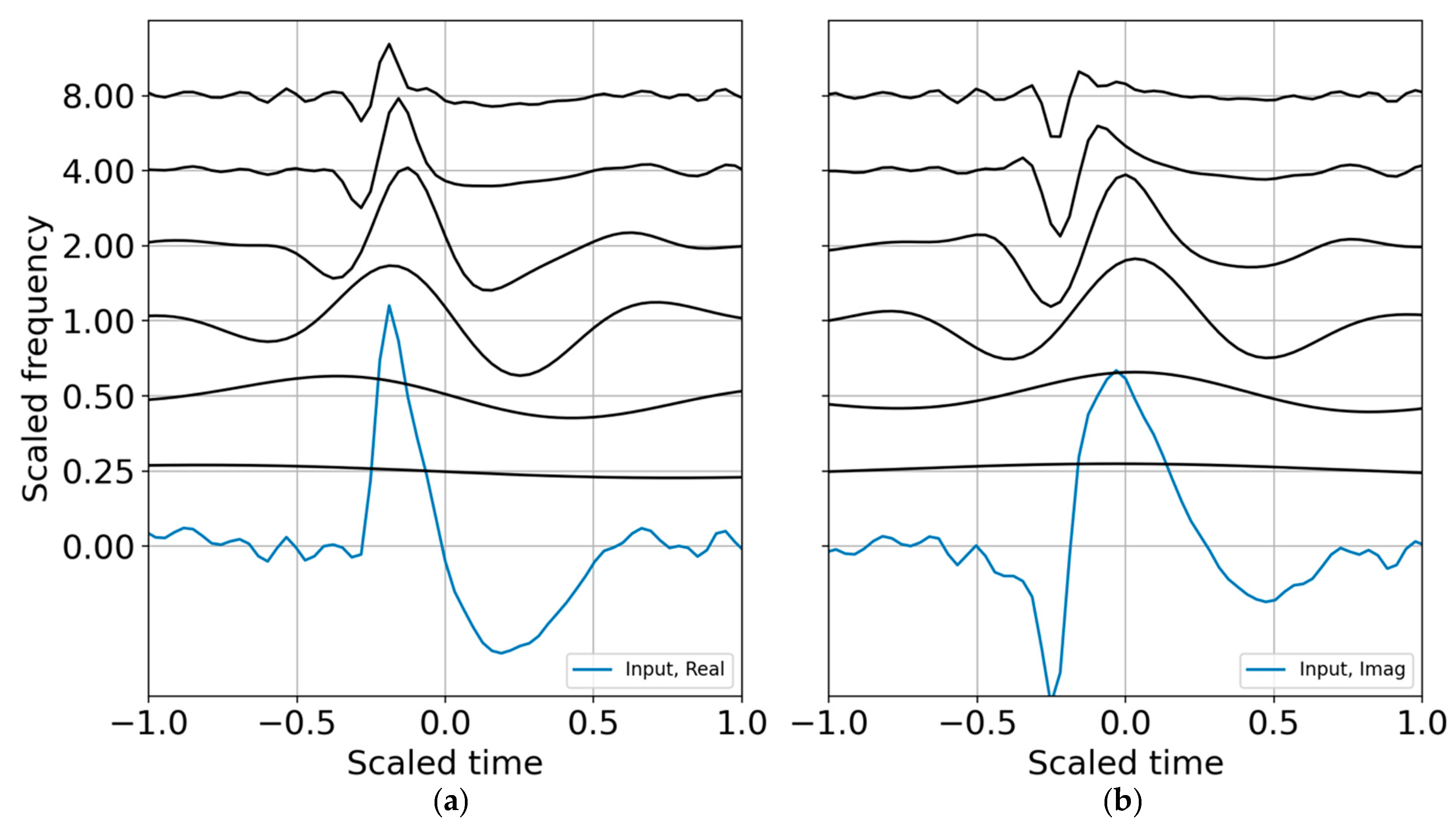
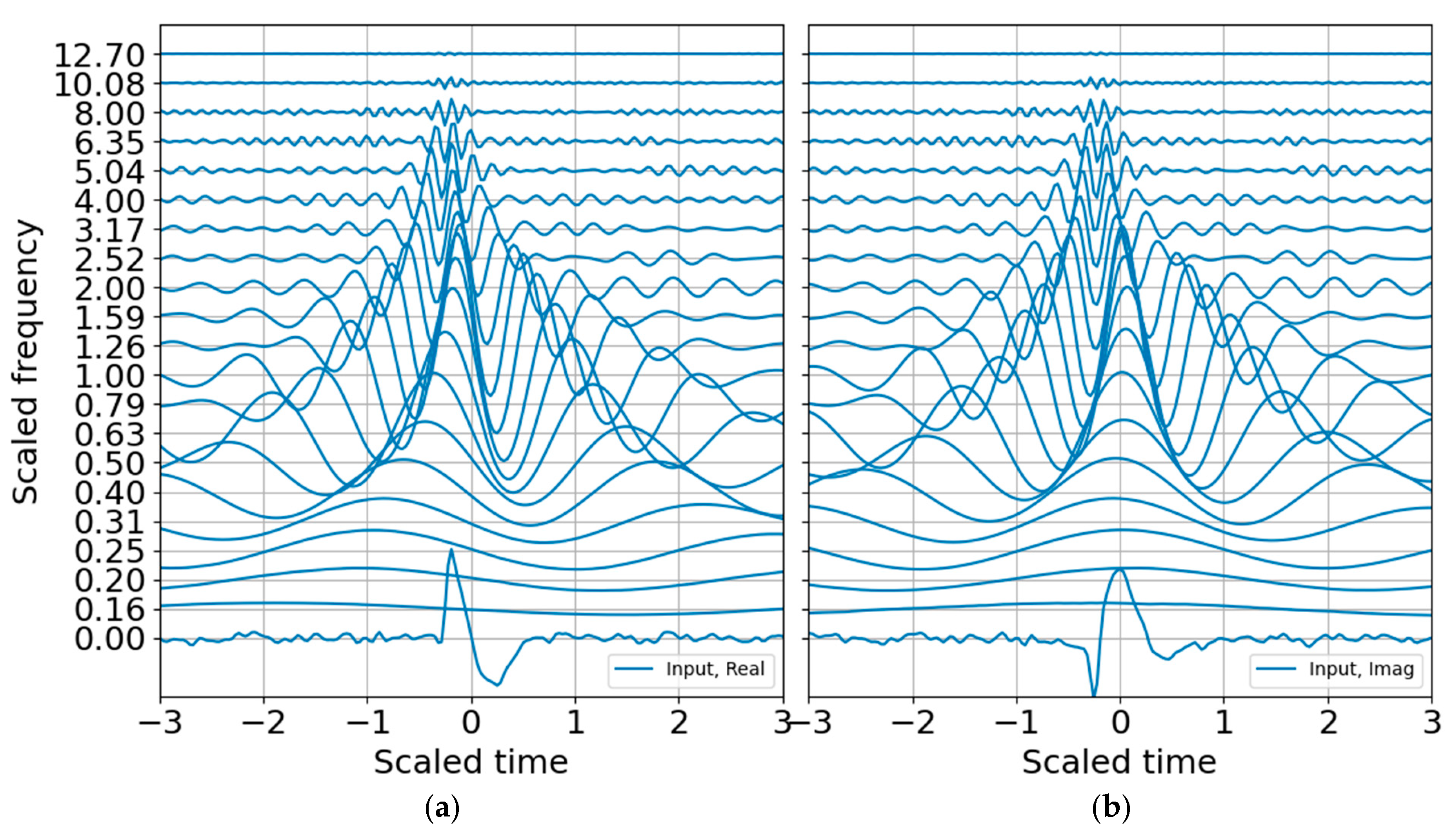
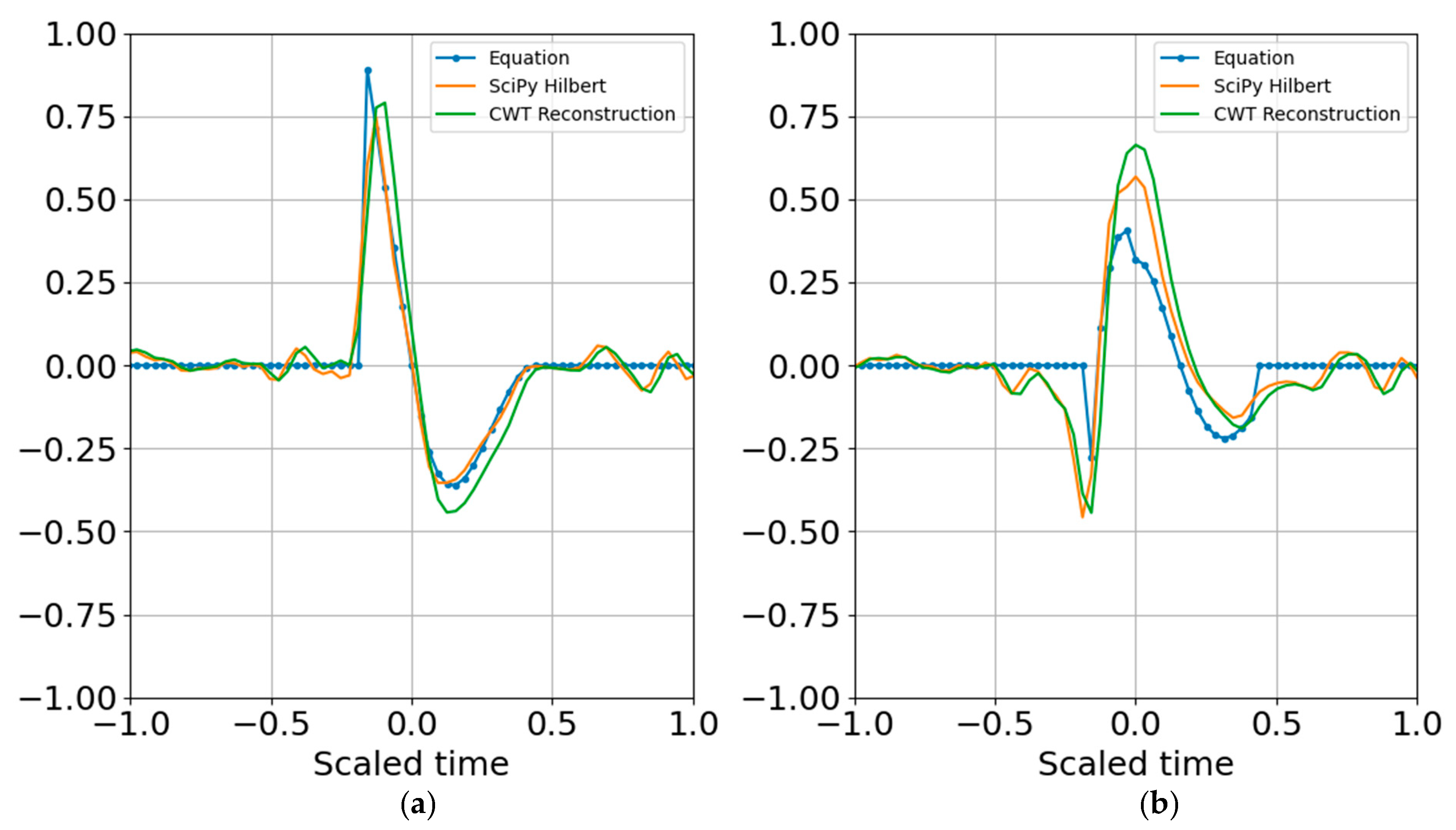
where the $i,j$ indexes indicate that one may choose selected scales for the reconstruction over selected time indexes $m_k:m_l$ corresponding to the wavelet coefficients that best represent a signal of interest during the time interval of relevance. The wavelet CWT coefficients for the binary band decomposition are shown in Figure 1; the CWT coefficients are scaled by the reconstruction coefficients. A comparison of the input synthetic analytic record and the analytic signal reconstruction (summed over all scales) for the octave band representation is shown in Figure 2.

The reconstruction process recovers the original dimensionality of the time series but returns its Hilbert transform, so the total dimensionality may be doubled (2Mp sample points). If only the original real signal is desired, then the dimensionality is unchanged.

The next steps estimate entropy and SNR, and consider sparse signal representation. Although binary bands are adequate for characterizing this signal, and are routinely used in the discrete wavelet transform, I take advantage of the flexibility offered by the CWT and use third order bands (N = 3) for the examples that follow. One of the benefits of third order bands is that the admissibility condition is better met and scales are recursive in powers of 2 and 10 ([1]). 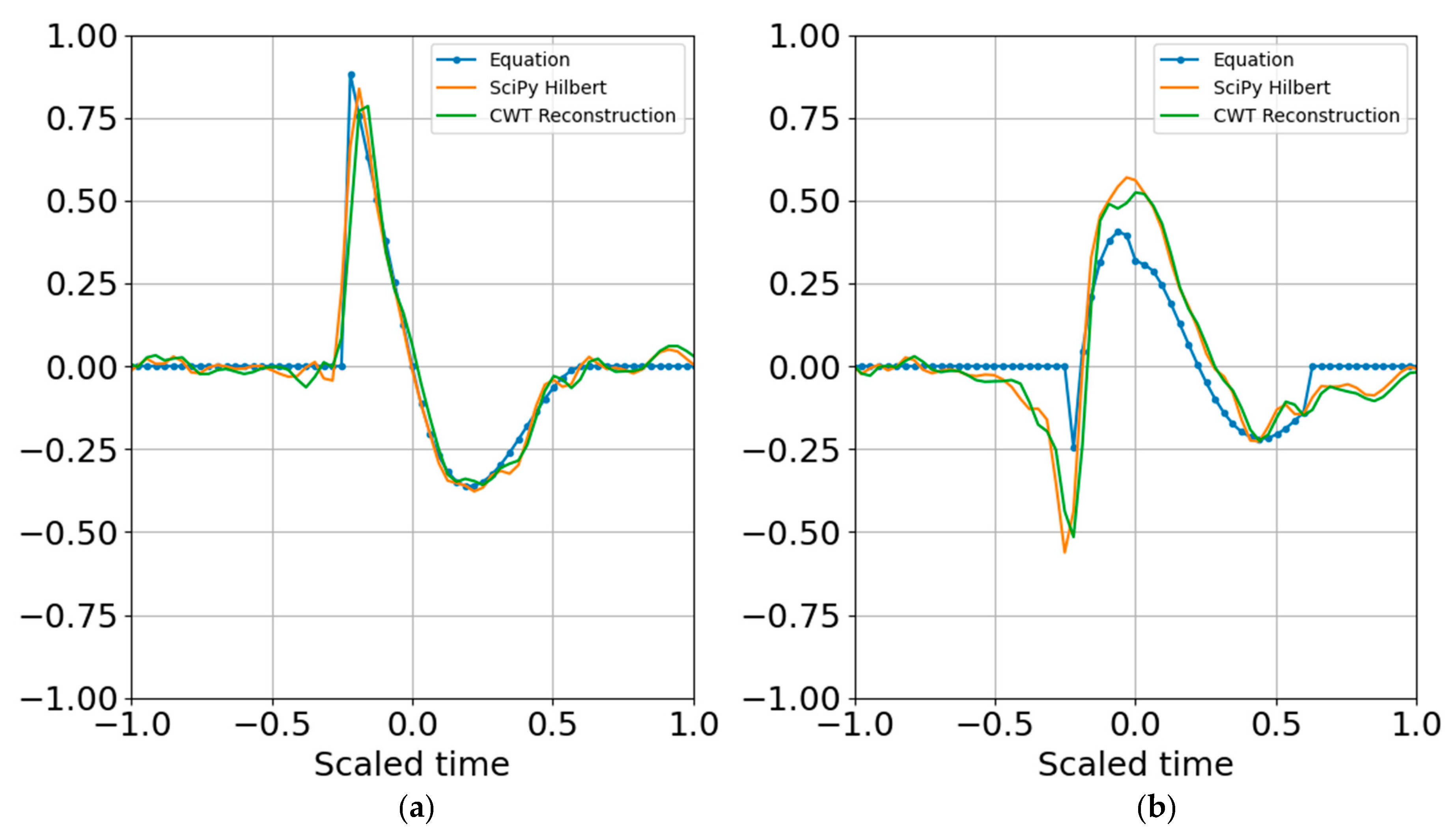As presented in Appendix D, third order bands will contain over 99% of the Gabor box variance within an octave and within 80% of the full window $T_n$, reducing spectral leakage. If, in addition, one wants a factor of two accuracy in explosive yield estimates, 1/3 octave resolution is a minimum requirement. 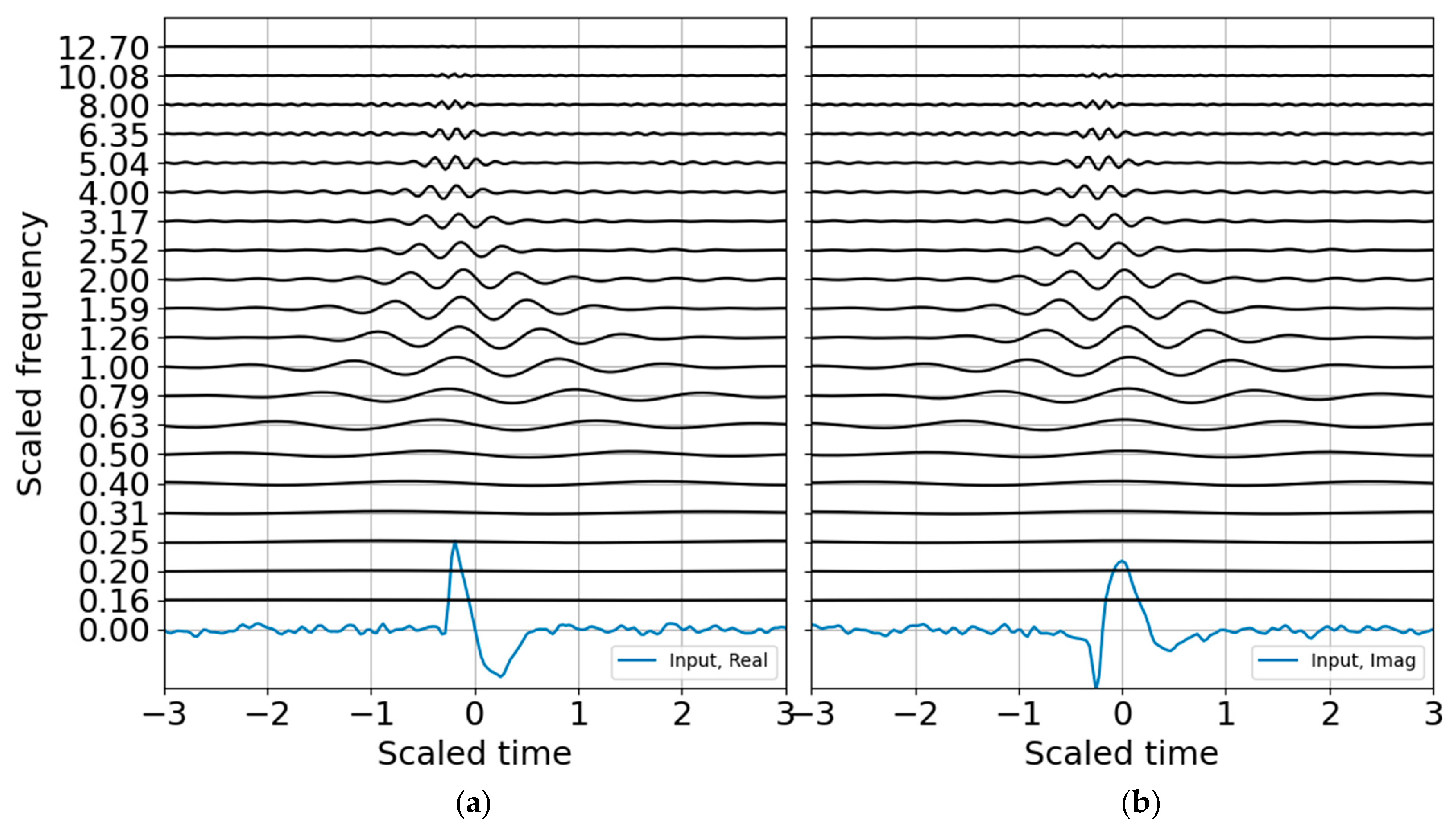A third order band wavelet reconstruction is shown in Figure 3 and corresponds to the CWT decomposition presented in Figure 4. The wire mesh representation is the equivalent of the scalograms usually represented as color mesh plots, and illustrates the simplicity of the CWT decomposition. The primary difference between Figure 4 and Figure 5 is that the first scales the raw CWT coefficients by the reconstruction scaling, whereas Figure 5 shows the raw coefficients.

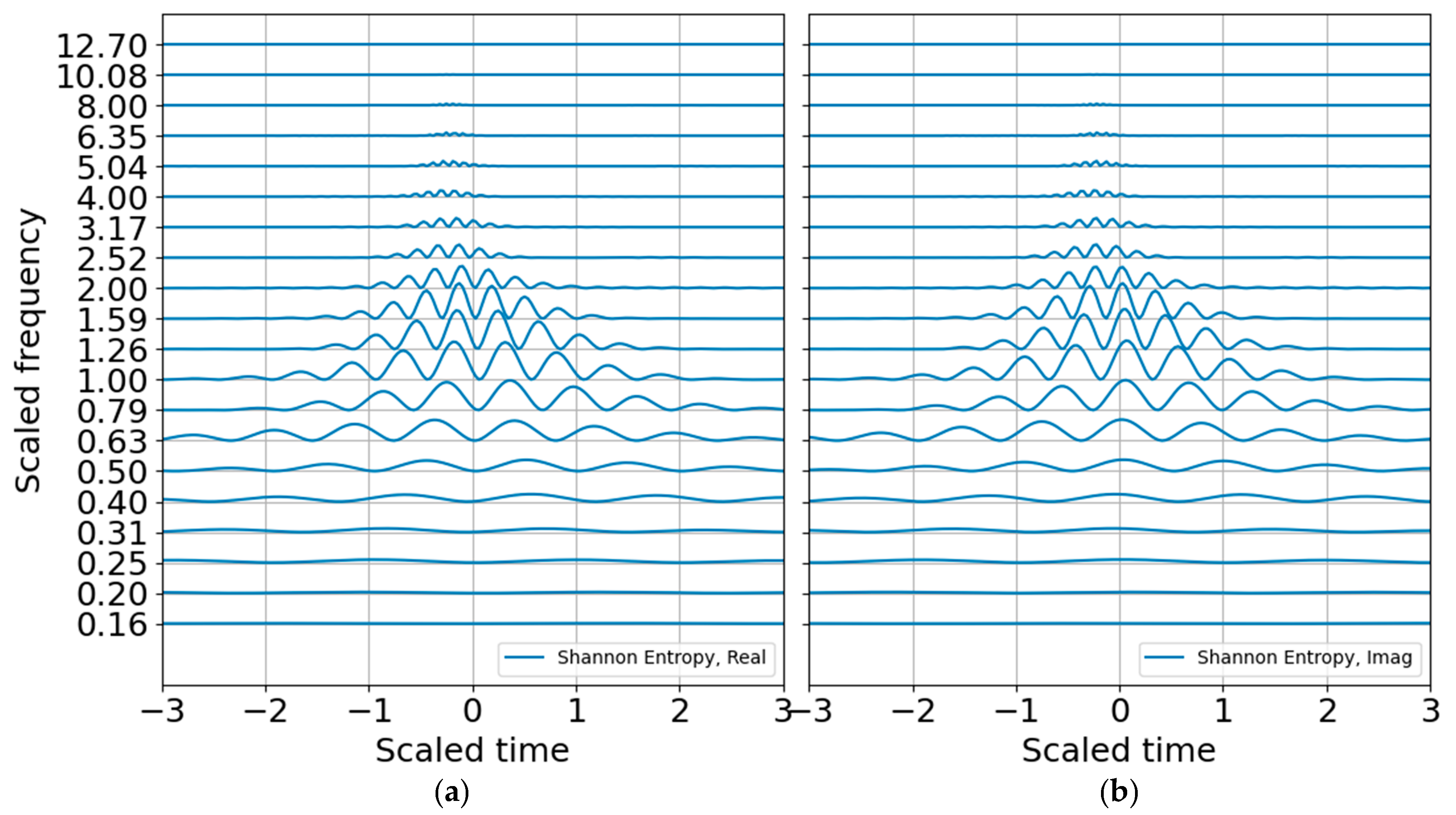
The energy probability distribution is constructed from the wavelet coefficients to estimate entropy, as discussed in the previous section. The log energy entropy looks like any other scalogram and does not add much value, but the Shannon entropy plot is interesting and well scaled (Figure 6). The peak entropy is at the scaled blast center frequency of unity, as expected.

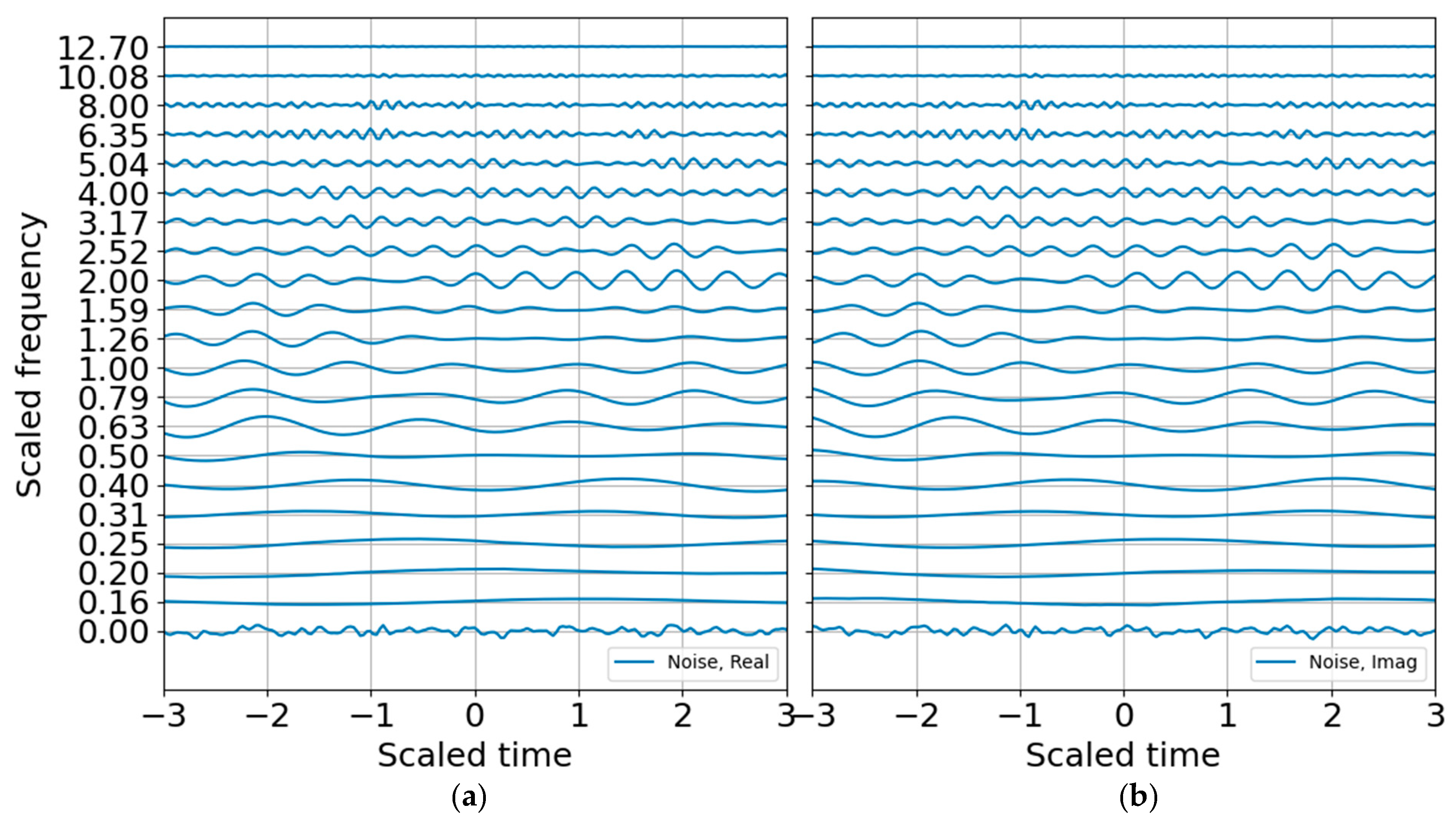
Next a noise model is constructed to build the SNR and to establish criteria for standardized and reproducible sparse signal representation. Many are the ways to characterize noise, and few of them accurately characterize non-stationary noise over brief observation windows. An incorrect noise model can penalize the signal passband and degrade the signal SNR. For the white noise model with variance that is one bit below the signal variance, the CWT of the noise (Figure 7) shows how the high-frequency oscillations are adequately sampled whereas the low-frequency oscillations are undersampled. This leads to instability if the noise is only estimated over a brief observation record. In principle, one may build a noise model over a substantial time period to improve statistical significance under the assumption that the noise is statistically stationary. This can be a tenuous assumption in some circumstances. Noise studies are beyond the scope of this paper; the noise spectrum is flattened by using the mean of the noise coefficients to estimate the band-averaged noise level.

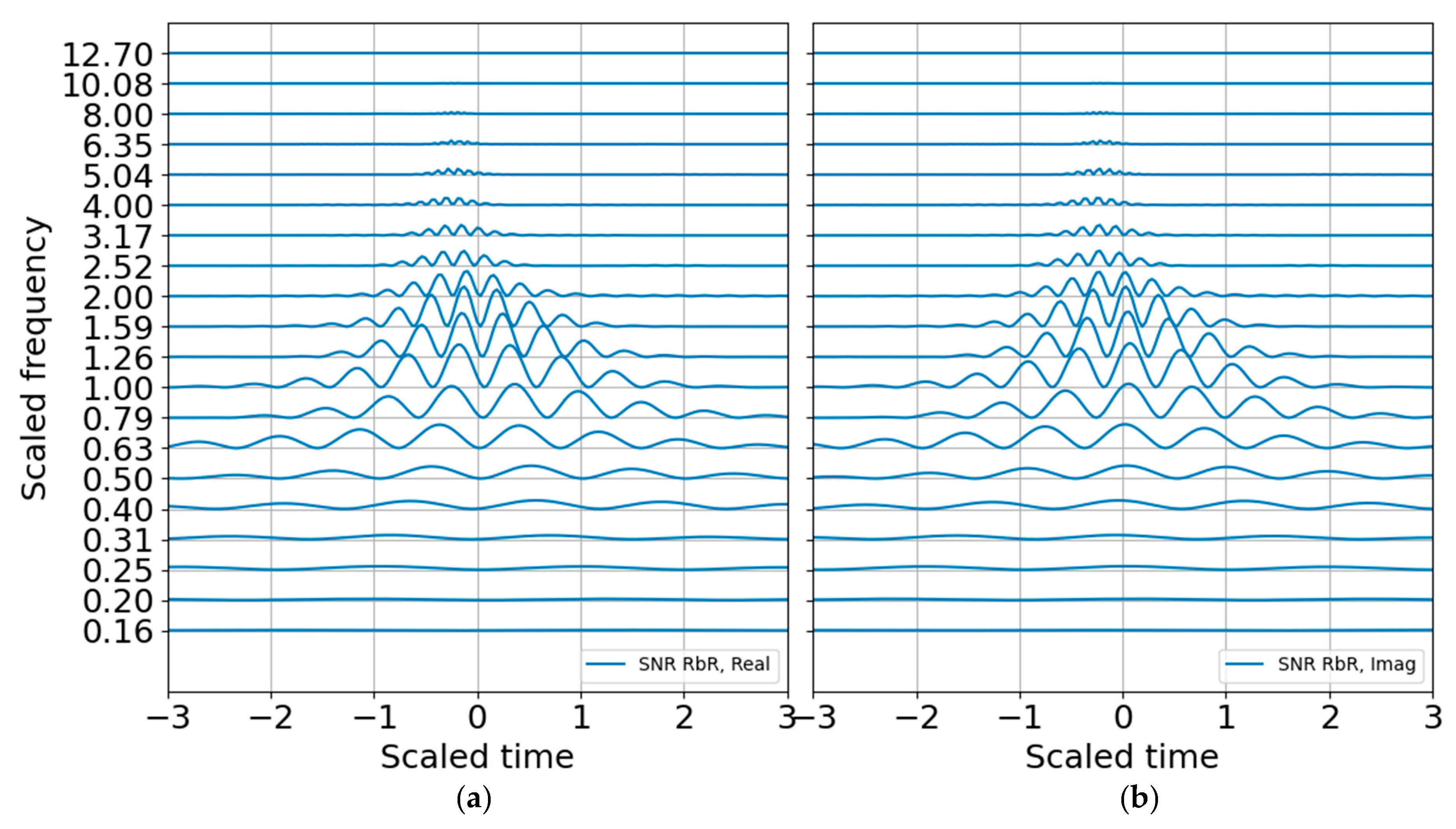
As anticipated, the binary SNR appears much like the log energy entropy since they are both scaled by a constant value, with the former over the band-averaged noise and the latter over the total energy. The SNR RbR, as described in the previous section, should also look very much like the entropy, except it would be zero for SNR of unity and positive for SNR > 1. The SNR RbR is shown in Figure 8 and indeed matches the Shannon entropy plot. This is encouraging; the entropy plot requires constructing an energy distribution that scales with the record, whereas the SNR requires constructing a noise model that is mostly independent of the record and should have more stability—as long as the ambient noise is approximately stationary or can at least be adequately modeled. If one is curating data for machine learning training, the entropy would be a good metric for picking and annotating possible signals as well as for refining noise models. If one is trying to trigger or detect signals operationally, the SNR may be a preferable metric since it makes no assumptions about the total energy in a record and only scales relative to a (preferably) stable noise representation.

One may use the CWT coefficient energy, the Shannon entropy, or the SNR RbR to test the feasibility of the sparse Gabor atom superposition. Suppose we use any of these Np scales x Mpoint time matrices to identify the peak contributions over the record, and define the complex time indexes as $m_{ℂmax}$. The quantum wavelet superposition would be expressed as

$$g_{ℂij}\left[m_k:m_l\right]\approx \frac{{\pi }^{\frac{1}{4}}}{2}{\displaystyle \sum }_{n=i}^j\frac{{\mathcal{W}}_n\left[m_{nℂmax}\right]}{\sqrt{{𝓈}_n}}Re\left\{{\mathsf{\Psi }}_n\left[m_k:m_l-m_{nℂmax}\right]\right\}$$

(88)

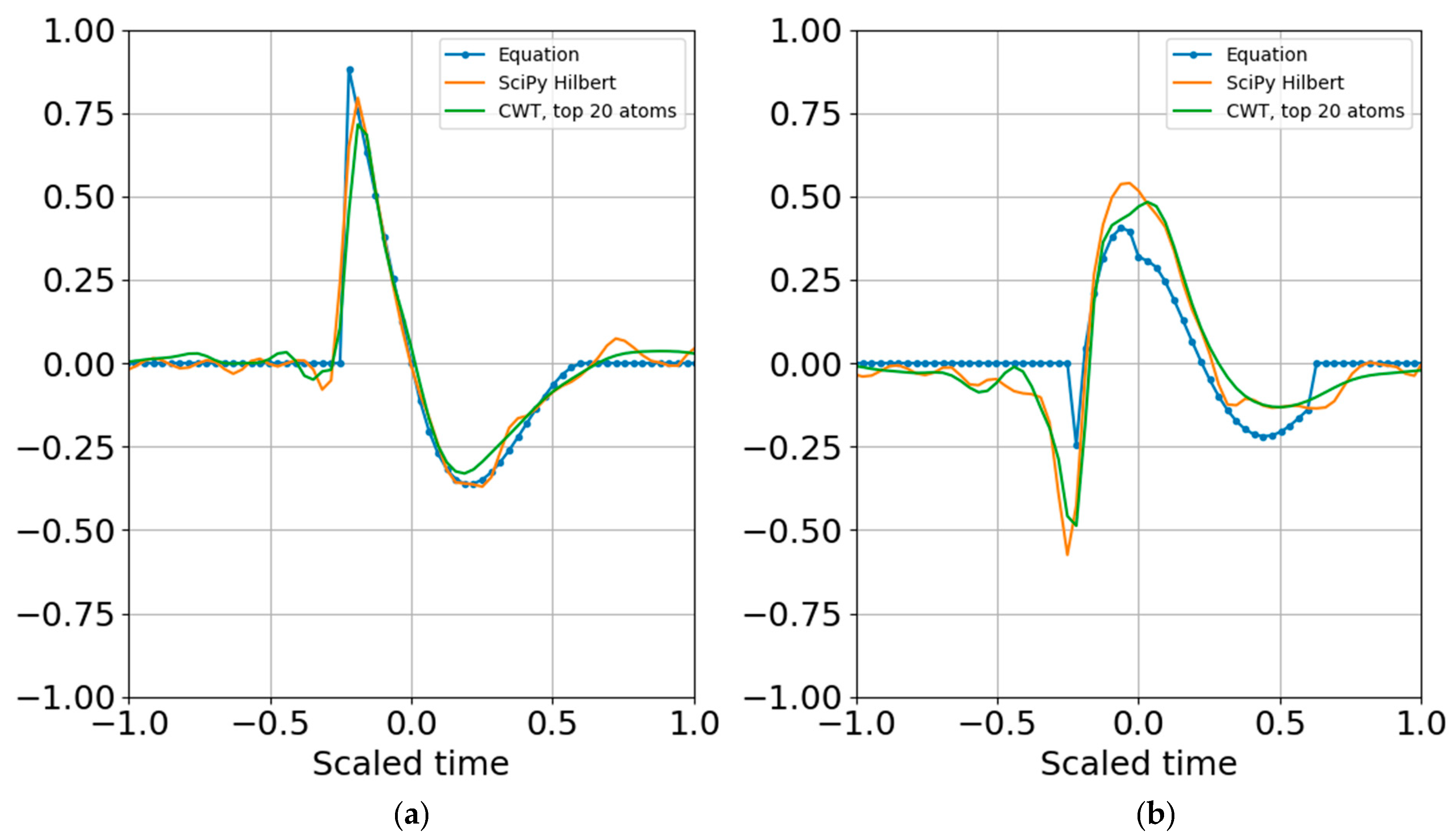
where the dimensionality of the representation is reduced to the complex coefficients and time indexes. Since the wavelet function can be reproduced for any time index, the time array need not be stored. In other words, if there are 20 scales, there will be 20 real coefficients and time offsets and 20 imaginary coefficients and time offsets, with total dimensionality of 4 × 20 = 80 parameters. If there is sufficient SNR and the signal is band limited it is possible to further reduce dimensionality by removing any coefficients below a specified threshold that may be fitting to noise (e.g., overfitting). 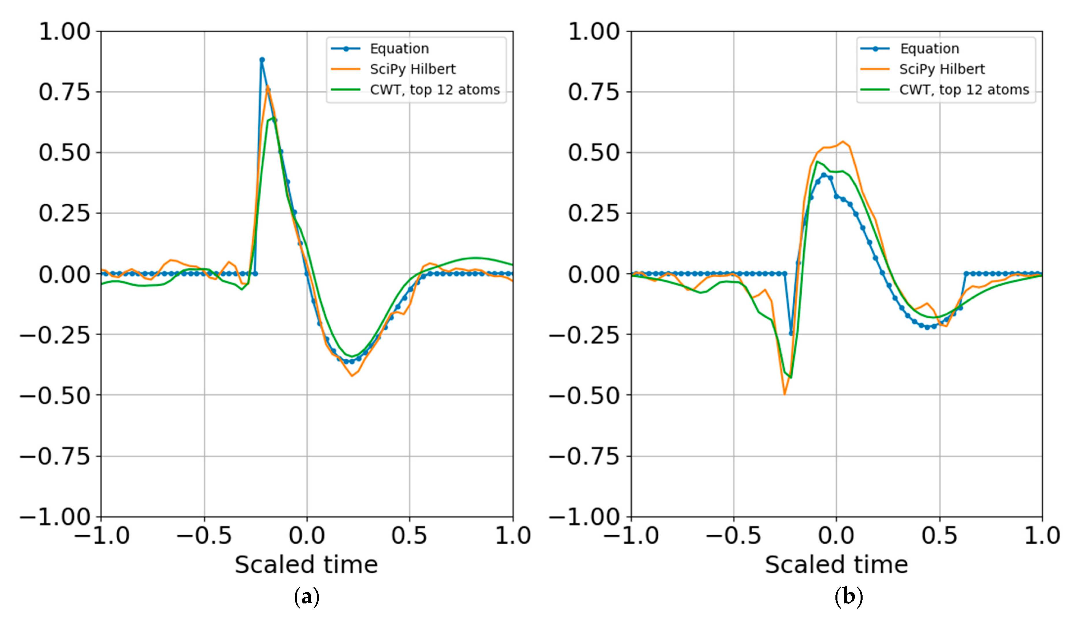Figure 9 shows the result of reconstruction from the superposition of all the top atoms of the 20 scales, and Figure 10 shows reconstruction from a sparser set of 12 scales with the highest SNR RbR. Similar results were obtained using the Shannon entropy. The Gaussian noise standard deviation for these two runs was one bit below the signal standard deviation.

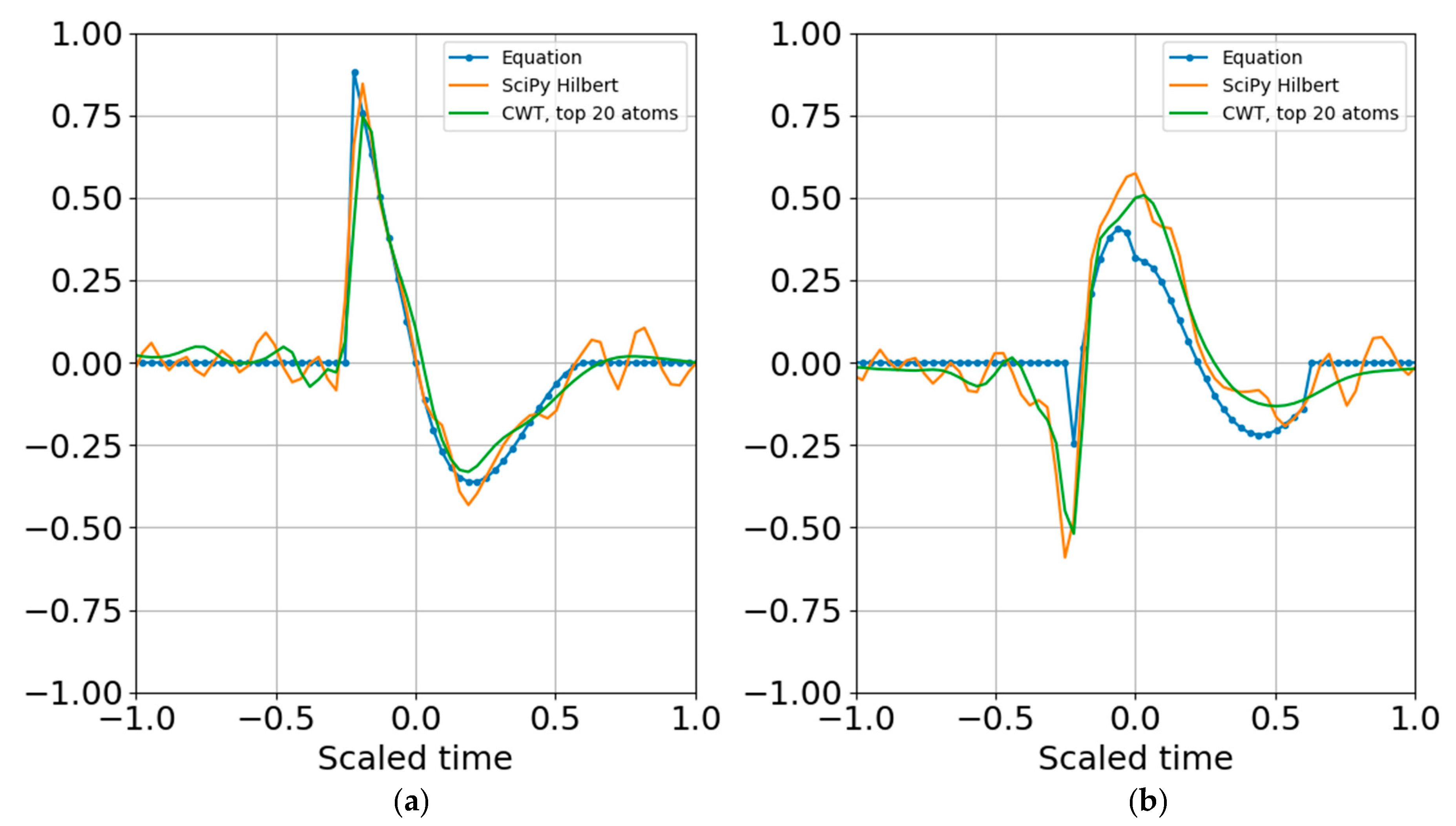
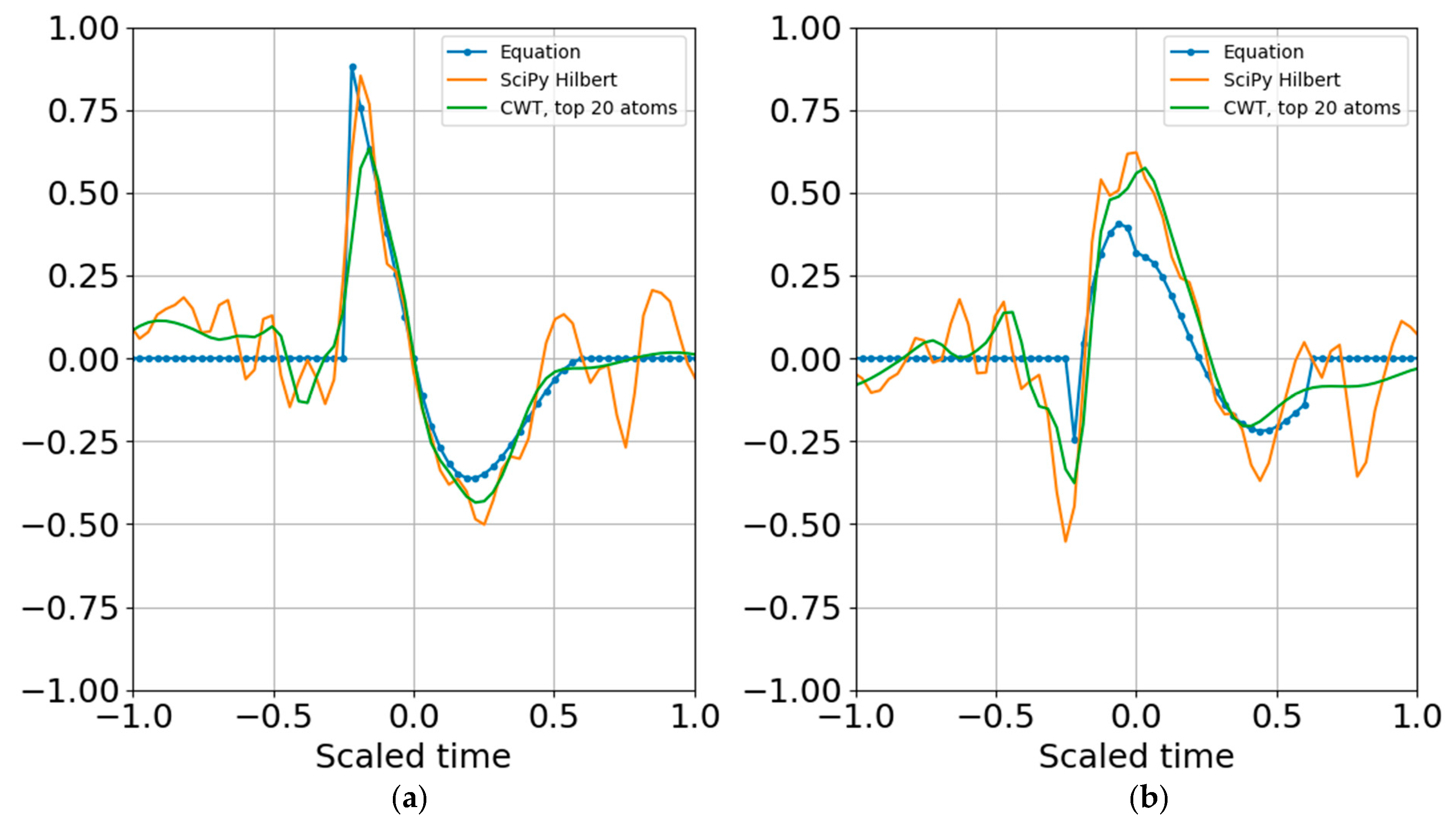
Increasing the noise standard deviation by a factor of two (one bit) still permits reconstruction from superposition (Figure 11), and increasing by another bit also allowed atomic reconstruction (Figure 12).

There is no end to the number of sensitivity studies that can be performed; in addition to other SNR tests, shifting the peak blast frequency away from the nominal target frequency still returned a stable reconstruction. Increasing the order past N > 6 only worsened the fit to the target waveform, increasing dimensionality and computational cost while decreasing reconstruction fidelity. This is expected from using a wavelet that does not match the target signature.

4. Concluding Remarks

This paper proposes a transition to binary metrics for digital data and introduces a standardized, quantized variation of the Gabor atoms with binary bases, optimal time-frequency resolution, and clear spectral energy containment. A binary entropy-like metric for the SNR is proposed and used to extract the peak coefficients to evaluate the performance of the superposition of Gabor atoms against the more traditional CWT reconstruction. Although the immediate application is the analysis of time series data collected with cyber-physical systems such as smartphones, the methods presented in this paper should be transportable to other types of digital records and can be extended to other wavelet families.

I used a synthetic pressure pulse corresponding to the detonation of one metric ton if TNT in Gaussian noise as an example, and did not include the blast amplitude as a key parameter in order to concentrate on the entropy and SNR, which are both dimensionless scaled quantities. Observations collected close to an explosion should have brief durations and a high SNR; for short pulses it is advisable to use Gabor atoms of small order (N = 1 − 6). Due to cube root yield scaling, the third order bands will provide a yield resolution—and uncertainty—of a factor of two, and one-sixth order bands will return square root of two yield resolution. In other words, the uncertainty of yield estimates obtained with the quantum wavelet would be inversely proportional to the cube root of the band order. Acceptable signal reconstructions were obtained from the CWT coefficients as well as the superposition of the peak third order Gabor atoms for the blast signature. At increasing distance from the source, the peak frequency is expected to drop [7] and the pulse disperses over time. This opens up the possibility for stable 6 and 12 order analyses with a corresponding improvement in yield resolution. Future work will concentrate on such dispersed signatures as well as consider other types of CW signatures that would be well matched to higher-order Gabor atoms.

The methods developed have the goal of providing a tunable, standardized framework for signature feature extraction that can be used for signal classification and which should be well suited for dictionary learning [13].