Modelling of Chaotic Processes with Caputo Fractional Order Derivative

Abstract

Chaotic dynamical systems are studied in this paper. In the models, integer order time derivatives are replaced with the Caputo fractional order counterparts. A Chebyshev spectral method is presented for the numerical approximation. In each of the systems considered, linear stability analysis is established. A range of chaotic behaviours are obtained at the instances of fractional power which show the evolution of the species in time and space.

1. Introduction

Fractional differential systems are largely encountered in various fields of applied sciences and engineering [1,2,3,4,5]. The study of differential equations of noninteger-order derivative have made tremendous development in terms of theory and application. It encompasses the general extension of classical order integrals and derivatives to fractional order counterparts.

The concept of fractional derivative has greatly been extended to various fractional ordinary differential equations, for instance the fractional Sturm–Liouville, Cauchy, and Gauss equations [1], with lots of applications in modelling of partial differential equations such as the complex cubic-quintic Ginzburg–Landau equation, Gray–Scott system [6], Burgers equation, Fisher equation, Fokker–Planck equation [7], and a range of fractional advection-reaction-diffusion problems, see [1,3,8] and references given therein. The main advantage of such models is the introduction of a fractional parameter, say $\gamma$ which can be used to model non-Markovian behaviour of spatial or temporal processes. This technique has emerged over the years as generalisations of many classic scenarios in mathematical physics.

Over the years, it is understood that many phenomena in application areas of science can be analysed successfully by models with the aid of mathematical tools from fractional calculus. A lot of researchers have realised the importance of fractional differential equations in describing real-life phenomena. A large number of fractional models have been suggested and examined in different areas such as the merits of non-integer order equations over the integer-order cases, analytical results, numerical techniques, and a host of others.

Fractional differential equations have been studied by many researches with different methods of solutions [1,2,9]. Many authors have also investigated analytic results based on the existence and uniqueness of solutions to fractional differential equations [1,3,10]. It should be mentioned that most fractional differential models encountered in science and engineering do have exact solutions and as a result, a viable and approximate numerical technique is required. So, to find efficient and accurate numerical methods to handle this class of problems has been a challenge over the years. Among several analytic and numerical methods that have been proposed includes the Adomian decomposition method, finite difference technique, the homotopy-perturbation approach, predictor-corrector method, collocation spectral method, Fourier spectral method, among several others [11,12,13].

The aim of the present paper is to approximate a chaotic process using the Chebyshev spectral method. Various chaotic processes have been modelled by a number of fractional derivatives. Chaotic differential equations are largely encountered in various fields of engineering, physics, chemistry, economics, and other related applied science subjects [14,15,16]. The main advantage of spectral methods relies mainly in their accuracy for a given number of unknowns. For smooth problems especially in geometries, spectral methods offer exponential rates of convergence with good spectral accuracy [6,11,17,18].

The remainder part of this paper is structured as follows. Some mathematical preliminaries based on basic definitions of fractional calculus and some important properties of Chebyshev spectral polynomials are introduced in Section 2. The derivation of an approximate formula for a chaotic system is given in Section 3. Some numerical experiment to reveal the behaviour of such a system is reported in Section 4. The paper is concluded with the last section.

2. Useful Preliminaries

Some useful definitions, results, and properties of fractional calculus, and Chebyshev polynomials are reported in this section.

Given a general time-fractional differential equation:

$$\begin{array}{ccc}\hfill D^{\gamma }g\left(t\right)& =& f(t,D^{\beta }g\left(t\right)),\mathrm{for}1\le t>0,\hfill \\ \\ \hfill g^{\left(s\right)}\left(0\right)& =& {\sigma }_s,s=0,1,2,\dots ,n-1\hfill \end{array}$$

(1)

where $n-1<\gamma <n$ and $m-1<\beta <m$, for $m,n\in \mathbb{N},n-1\ge m$, $D^{\gamma }$ denotes the Caputo fractional derivative operator of order $\gamma$, and $f\in C\left(\right[0,1]\times \mathbf{R})$. For the existence of a solution, the nonlinear function f is required to satisfy the condition: ∃ two functions, say $a,b\in \left(\right[0,1],[0,\infty \left)\right):\forall 1\ge t\ge 0$ and for each $w\in \mathbf{R}$, we have $\left|f\right(t,w\left)\right|\le a\left(t\right)\left|w\right|+b\left(t\right)$. Similarly for the uniqueness result, the term f must satisfy the condition: $\exists a,b\in \left(\right[0,1],[0,\infty \left)\right):\forall 1\ge t>0$ and any $w,z\in \mathbf{R}$, we have $\left|f\right(t,w)-f(t,z\left)\right|\le a\left(t\right)|w-z|$.

The Caputo fractional derivative of order $\gamma >0$ is defined as:

$${}^C{\mathcal{D}}^{\gamma }g\left(x\right)=\frac{1}{\mathsf{\Gamma }(n-\gamma )}{\int }_0^x\frac{g^{\left(n\right)}\left(\tau \right)}{{(x-\tau )}^{\gamma -n+1}}d\tau ,$$

(2)

where $x>0$ and $n-1<\gamma \le n$ for $n\in \mathbb{N}$ and $\mathsf{\Gamma }\left(x\right)$ is the Gamma function.

The Caputo derivative of a constant is defined as:

$${}^C{\mathcal{D}}^{\gamma }A=0,\mathrm{with}A,\mathrm{a}\mathrm{constant}.$$

(3)

Also,

$${}^C{\mathcal{D}}^{\gamma }{x}^{\alpha }=\left\{\begin{array}{cc}0& \mathrm{for}\alpha \in {\mathbb{N}}_0\mathrm{and}\alpha <\lceil \gamma \rceil ,\\ \frac{\mathsf{\Gamma }(\alpha +1)}{\mathsf{\Gamma }(\alpha +1-\gamma )}{x}^{\alpha -\gamma }& \mathrm{for}\alpha \in {\mathbb{N}}_0\mathrm{and}\alpha \le \lceil \gamma \rceil .\end{array}\right.$$

(4)

Theorem 1

([10]). Let $m-1<\beta <\gamma <m$ for $m\in \mathbb{N}$. Assume that the following hypothesis holds: ($h_1$) $g:[0,1]\times \mathbf{R}\to \mathbf{R}$ is a continuously differentiable function, ($h_2$) $g(0,0)=0$ and $g(t,0)\ne 0$ on a compact subinterval of (0,] and ($h_3$) there exist $ϵ>1$, $1>\rho >0$ and $f\left(t\right)\in C\left(\right[0,1],[0,\infty \left]\right)$ such that:

$$\frac{1}{\mathsf{\Gamma }(\gamma -\beta )}\underset{0\le t\le 1}{sup}{\int }_0^t{(t-\tau )}^{\gamma -\beta -1}f\left(\tau \right)d\tau \le 1-\rho .$$

$$0<R:=\frac{1}{\mathsf{\Gamma }(\gamma -\beta )}\underset{0\le t\le 1}{sup}{\int }_0^t{(t-\tau )}^{\gamma -\beta -1}\left|g(\tau ,0)\right|d\tau <\infty$$

and for every $a,b\in C\left(\right[0,\infty \left]\right)$ with $0\le \left|a\left(t\right)\right|,\left|b\left(t\right)\right|\le \frac{1}{\rho }R$ for $1\ge t\ge 0$, then:

$$\left|g\right(t,a\left(t\right))-g(t,b\left(t\right)\left)\right|\le f\left(t\right)\left|a\right(t)-b(t\left)\right|\mathrm{for}1\ge t\ge 0.$$

Then Equation (1) has a unique solution.

For details of a similar proof of Theorem 1, see [10,19].

The Chebyshev polynomial on interval $[-1,1]$ is determined using the recurrence formula [12,20]:

$$G_{n+1}\left(x\right)=2x{G}_n\left(x\right)-G_{n-1}\left(x\right),G_0\left(x\right)=1,G_1\left(x\right)=x,\mathrm{for}n=1,2,\dots$$

The analytic form of the Chebyshev polynomials $G_n\left(x\right)$ is defined by:

$$G_n\left(x\right)=n\sum _{k=0}^{\lfloor \frac{n}{2}\rfloor }{(-1)}^k{2}^{n-2k-1}\frac{(n-k-1)!}{k!(n-2k)!}{x}^{n-2k},n=2,3,\dots ,$$

(5)

where $\lfloor \frac{n}{2}\rfloor$ stands for the integer case of $n/2$. The orthogonality property is given:

$${\int }_{-1}^1\frac{G_k\left(x\right)G_s\left(x\right)}{\sqrt{1-x^2}}dx=\left\{\begin{array}{cc}\pi & \mathrm{for}k=s=0,\\ \frac{\pi }{2}& \mathrm{for}k=s\ne 0,\\ 0& \mathrm{for}k\ne s,\end{array}\right.$$

(6)

It is necessary to introduce a change of variable $x=2t-1$ to enable us to apply the Chebyshev polynomial on interval $[0,1]$. Hence, we follow [12] and define the shifted Chebyshev polynomial as:

$$G^{*}\left(t\right)=G_n(2t-1)=G_{2n}\left(\sqrt{t}\right),$$

and its analytic form is given by:

$$G_n^{*}\left(t\right)=n\sum _{r=0}^n{(-1)}^{n-r}\frac{(n+r-1)!}{\left(2r\right)!(n-r)!}{t}^r,n=2,3,\dots$$

(7)

3. Fractional-Order Chaotic Systems and Formulation of Approximate Scheme

In this section, we introduce a three- and four-scroll chaotic attractor systems [21,22] and examine their linear stability analysis. Later, we derive an approximate formula based on the Chebyshev spectral method for their numerical approximations.

3.1. Chaotic System

Two important chaotic systems which exist in classical order forms, which have been studied and applied in various areas of finance, stock exchange, cryptology, population dynamics, etc. are reformulated here in the sense of the Caputo fractional order models. Each system is also examined for linear stability analysis.

3.1.1. Three Dimensional Fractional Chaotic System

The fractional order chaotic system of three components is described by the following differential equations [23]:

$$\begin{array}{ccc}\hfill {}^C{\mathcal{D}}_t^{\gamma }u\left(t\right)& =& f_1(u,v,w)=a_1(u\left(t\right)-v\left(t\right)),\hfill \\ \hfill {}^C{\mathcal{D}}_t^{\gamma }v\left(t\right)& =& f_2(u,v,w)=-4a_{1}v\left(t\right)+u\left(t\right)w\left(t\right)+a_2{u}^3\left(t\right),\hfill \\ \hfill {}^C{\mathcal{D}}_t^{\gamma }w\left(t\right)& =& f_3(u,v,w)=-a_1{a}_{4}w\left(t\right)+u^3\left(t\right)v\left(t\right)+a_3{w}^2\left(t\right),\hfill \end{array}$$

(8)

where $u\left(t\right),v\left(t\right)$ and $w\left(t\right)$ denote state variables and $a_i>0$ for $i=1\left(1\right)4$ are parameters.

To examine system (8) for equilibrium points, we set ${}^C{\mathcal{D}}_t^{\gamma }=f_i(u,v,w)=0,i=1,2,3$. That is,

$$\begin{array}{ccc}\hfill 0& =& a_1(u\left(t\right)-v\left(t\right)),\hfill \\ \hfill 0& =& -4a_{1}v\left(t\right)+u\left(t\right)w\left(t\right)+a_2{u}^3\left(t\right),\hfill \\ \hfill 0& =& -a_1{a}_{4}w\left(t\right)+u^3\left(t\right)v\left(t\right)+a_3{w}^2\left(t\right).\hfill \end{array}$$

(9)

With this development, it is obvious that system (8) has four steady states, which correspond to $E_0=(0,0,0)$ which is the washout state, $\overline{E}=(0,0,\frac{a_1{a}_4}{a_3})$, this point corresponds to the existence of state variable w only. The other two equilibrium points are given by:

$$E_{+}^{*}=\left(\sqrt{\frac{4a_1-w^{*}}{a_2}},\sqrt{\frac{4a_1-w^{*}}{a_2}},\frac{a_1(a_4{a}_2^2+8)+a_1{a}_2\sqrt{a_4^2{a}_{2}2+16a_4-64a_3}}{2a_3{a}_2^2+2}\right)$$

and

$$E_{-}^{*}=\left(-\sqrt{\frac{4a_1-w^{*}}{a_2}},-\sqrt{\frac{4a_1-w^{*}}{a_2}},\frac{a_1(a_4{a}_2^2+8)+a_1{a}_2\sqrt{a_4^2{a}_{2}2+16a_4-64a_3}}{2a_3{a}_2^2+2}\right)$$

where $w^{*}=\frac{a_1(a_4{a}_2^2+8)+a_1{a}_2\sqrt{a_4^2{a}_{2}2+16a_4-64a_3}}{2(a_3{a}_2^2+1)}$. The Jacobian or community matrix of system (8) corresponds to:

$${\mathbf{A}}_{u,v,w}=\left(\begin{array}{ccc}{a}_1& -a_1& 0\\ 3a_2{u}^2+w& -4a_1& u\\ 3u^{2}v& u^3& 2a_{3}w-a_1{a}_4\end{array}\right).$$

(10)

Let $det(\lambda I-\mathbf{A}(0,0,0\left)\right)=0$, we obtain the characteristic equation:

$${\lambda }^3+k_1{\lambda }^2+k_2\lambda -k_3,$$

where $k_i,i=1,2,3=(1.8,1.61,35)$, respectively. Clearly on solving further, we obtain the eigenvalues as ${\lambda }_1=toe1.80,{\lambda }_2=-7.20$, and ${\lambda }_3=-7.20$. Since one of the roots of the characteristic equation above is a positive real number, the remaining two are real-negative, then point $E^0$ is saddle and unstable. Following a similar procedure, the corresponding eigenvalues at point $\overline{E}$ as ${\lambda }_1=6.77$, ${\lambda }_2=-12.17$ and ${\lambda }_1=2.70$, therefore since one of the three eigenvalues has an opposite sign, the point $\overline{E}$ is also unstable.

Next, by considering the interior point $E_{\pm }^{*}$, we have eigenvalues $({\lambda }_1,{\lambda }_2,{\lambda }_3)=(0.83-3.83j,0.83+3.83j,-10.75)$ and $({\lambda }_1,{\lambda }_2,{\lambda }_3)=(0.83-3.83j,0.83+3.83j,-10.75)$, respectively. In both equilibrium points $E_{+}^{*}$ and $E_{-}^{*}$, we have ${\lambda }_3$ as a negative real number, whereas ${\lambda }_1$ and ${\lambda }_2$ are a conjugate pair of complex eigenvalues with positive real parts. This indicates that the nontrivial points $E_{+}^{*}$ and $E_{-}^{*}$ are saddle-focus. Hence, these steady states are unstable points.

To analyse the nonlinear behaviour of the dynamic system (8), we consider its Lyapunov exponent, which measures the exponential rates of divergence or convergence of trajectories. It should be mentioned that if at least one of the Lyapunov exponent (LE) is positive, then we have a chaotic system. With parameters $a_1=1.8,a_2=0.12,a_3=-0.07;a_4=1.5;$ and $a_4=1.5$ with $(u_0,v_0,w_0)=(2.6,1.8,2.5)$, we get the corresponding as $L{E}^1=-2.679038,L{E}^2=-2.692823$, and $L{E}^3=-8.113770,t=100.0000-2.679038-2.692823-8.113770$. Please see Figure 1) for the dynamic of Lyapunov exponents computed at $t=100$. Figure 2, Figure 3 and Figure 4 shows the chaotic evolution of fractional system (8) for $\gamma =0.38$, $\gamma =0.51$ and $\gamma =0.99$, arbitrarily chosen.

3.1.2. Four-Scroll Fractional-Order Chaotic System

A four-scroll Caputo fractional order chaotic system with nine parameters is given as [21,22]:

$$\begin{array}{ccc}\hfill {}^C{\mathcal{D}}_t^{\gamma }u\left(t\right)& =& f_1(u,v,w)=b_{1}v\left(t\right)-b_{2}u\left(t\right)+b_{3}u\left(t\right)w\left(t\right),\hfill \\ \hfill {}^C{\mathcal{D}}_t^{\gamma }v\left(t\right)& =& f_2(u,v,w)=-b_{4}u\left(t\right)w\left(t\right)-b_{5}u\left(t\right)+b_{6}v\left(t\right)w\left(t\right)+b_{7}u\left(t\right),\hfill \\ \hfill {}^C{\mathcal{D}}_t^{\gamma }w\left(t\right)& =& f_3(u,v,w)=b_8-b_9{v}^2\left(t\right),\hfill \end{array}$$

(11)

with ${}^C{\mathcal{D}}_t^{\gamma }=f_i(u,v,w)=0$, the Caputo chaotic system (11) have equilibrium states:

$$(u,v,w)=E_{\pm }=({\overline{u}}_{\pm },{\overline{v}}_{\pm },{\overline{w}}_{\pm })$$

where,

$${\overline{u}}_{+}=\frac{b_1{\overline{v}}_{+}}{b_2-b3{\overline{w}}_{+}},{\overline{u}}_{-}=\frac{b_1{\overline{v}}_{-}}{b_2-b3{\overline{w}}_{-}},$$

$${\overline{v}}_{+}=\sqrt{\frac{b_8}{b_9}},{\overline{v}}_{-}=-\sqrt{\frac{b_8}{b_9}}$$

and

$${\overline{w}}_{+}=\frac{b_2{b}_6-b_1{b}_4}{2b_3{b}_6}+\frac{\sqrt{{(b_2{b}_6-b_1{b}_4)}^2-4b_1{b}_3{b}_6(b_5-b_7)}}{2b_3{b}_6},$$

$${\overline{w}}_{-}=\frac{b_2{b}_6-b_1{b}_4}{2b_3{b}_6}-\frac{\sqrt{{(b_2{b}_6-b_1{b}_4)}^2-4b_1{b}_3{b}_6(b_5-b_7)}}{2b_3{b}_6}.$$

The linear stability is obtained by solving the characteristic equation:

$${\lambda }^3+{\xi }_2{\lambda }^2+{\xi }_1\lambda +{\xi }_0=0,$$

(12)

where,

$${\xi }_2=b_2-\overline{w}(b_3+b_6),$$

$${\xi }_1=\frac{2b_9\overline{u}\overline{v}(b_5-b_7)}{\overline{w}},$$

and

$${\xi }_0=\frac{2b_8[b_1(b_5-b_7)-b_3{b}_6{\overline{w}}^2]}{\overline{w}}.$$

With $\varpi ={(b_2{b}_6-b_1{b}_4)}^2-4b_1{b}_3{b}_6(b_5-b_7)=0$, we have saddle-node bifurcation, when $\varpi >0$ we have two fixed points. One of the fixed points is stable while the other unstable for ${\overline{w}}_{\pm }$. Figure 5, Figure 6, Figure 7, Figure 8 and Figure 9 for $\gamma =1$, $\gamma =0.38$, $\gamma =0.50$, $\gamma =0.61$, and $\gamma =0.84$, arbitrarily chosen. Also Figure 10 shows the time series chaotic evolution of system (11) for several values of $\gamma$.

3.2. Formulation of Approximate Method

The function $g\left(t\right)$ in space $[0,1]$ can be defined in terms of shifted Chebyshev polynomials as:

$$g\left(t\right)=\sum _{k=0}^{\infty }{\omega }_k{G}_k^{*}\left(t\right),$$

(13)

with ${\omega }_k$ as coefficients, expressed in the form [20]:

$${\omega }_k=\frac{2}{\pi {\hslash }_k}{\int }_0^1\frac{g\left(t\right)G_k^{*}\left(t\right)}{\sqrt{t-t^2}}dt,{\hslash }_0=2,{\hslash }_k=1,k=1,2,\dots .$$

(14)

It is customary to consider only the first $(x+1)$ terms of the shifted Chebyshev polynomials. In such that:

$$g_x\left(t\right)=\sum _{k=0}^x{\omega }_k{G}_k^{*}\left(t\right).$$

(15)

The approximate formula for fractional derivative of order $\gamma >0$ of $g_x\left(t\right)$ using the above Chebyshev polynomials, to have:

$${\mathcal{D}}_t^{\gamma }\left(g_x\left(t\right)\right)=\sum _{k=\lceil \gamma \rceil }^x\sum _{r=\lceil \gamma \rceil }^k{\omega }_k{f}_{k,r}^{\left(\gamma \right)}{t}^{r-\gamma },$$

(16)

where,

$$f_{k,r}^{\left(\gamma \right)}={(-1)}^{k-r}\frac{2^{2r}k(k+r-1)!\mathsf{\Gamma }(r+1)}{(k-r)!\left(2r\right)!\mathsf{\Gamma }(r+1-\gamma )}.$$

So, the Caputo fractional operator of order $\gamma >0$ for the shifted Chebyshev polynomials is given in the form:

$${}^C{\mathcal{D}}_0^{\gamma }\left[G_k^{*}\left(t\right)\right]=\sum _{r=\lceil \gamma \rceil }^k\sum _{s=0}^{r-\lceil \gamma \rceil }{\chi }_{k,r,s}{G}_s^{*}\left(t\right),$$

(17)

where,

$${\chi }_{k,r,s}=\frac{{(-1)}^{k-r}2k(k+r-1)!\mathsf{\Gamma }(r-\gamma +\frac{1}{2})}{{\hslash }_s\mathsf{\Gamma }(r+\frac{1}{2})(k-r)!\mathsf{\Gamma }(r-\gamma -s+1)\mathsf{\Gamma }(r+s-\gamma +1)},\mathrm{for}s=0,1,2,\dots$$

The error, denoted as $|E_r\left(x\right)|$ is calculated as $|{\mathcal{D}}^{\gamma }g\left(t\right)-{\mathcal{D}}^{\gamma }{g}_x\left(t\right)|$ in approximating ${\mathcal{D}}^{\gamma }g\left(t\right)$ by ${\mathcal{D}}^{\gamma }{g}_x\left(t\right)$ which is bounded by:

$$|E_r\left(x\right)|\le \left|\sum _{k=x+1}^{\infty }{\omega }_k\left(\sum _{r=\lceil \gamma \rceil }^k\sum _{s=0}^{r-\lceil \gamma \rceil }{\chi }_{k,r,s}\right)\right|.$$

For details, readers are referred to [20].

Next, we provide a solution procedure of the Caputo fractional chaotic system by first approximating $u\left(t\right),v\left(t\right)$ and $w\left(t\right)$ as:

$$\begin{array}{c}\hfill u_n\left(t\right)=\sum _{k=0}^n{x}_k{G}_k^{*}\left(t\right),v_n\left(t\right)=\sum _{k=0}^n{y}_k{G}_k^{*}\left(t\right),w_n\left(t\right)=\sum _{k=0}^n{z}_k{G}_k^{*}\left(t\right).\end{array}$$

(18)

From Equations (8) and (16) we obtain:

$$\begin{array}{ccc}\hfill & & \sum _{k=\lceil \gamma \rceil }^n\sum _{r=\lceil \gamma \rceil }^k{x}_k{f}_{i,r}^{\left(\gamma \right)}{t}^{r-\gamma }=a_1\left(\sum _{k=0}^n{x}_k{G}_k^{*}\left(t\right)-\sum _{k=0}^n{y}_k{G}_k^{*}\left(t\right)\right),\hfill \\ & & \sum _{k=\lceil \gamma \rceil }^n\sum _{r=\lceil \gamma \rceil }^k{y}_k{f}_{i,r}^{\left(\gamma \right)}{t}^{r-\gamma }=-4a_1\sum _{k=0}^n{y}_k{G}_k^{*}\left(t\right)+\left(\sum _{k=0}^n{x}_k{G}_k^{*}\left(t\right)\right)\left(\sum _{k=0}^n{z}_k{G}_k^{*}\left(t\right)\right)\hfill \\ & & +a_2{\left(\sum _{k=0}^n{z}_k{G}_k^{*}\left(t\right)\right)}^3\hfill \\ & & \sum _{k=\lceil \gamma \rceil }^n\sum _{r=\lceil \gamma \rceil }^k{z}_k{f}_{i,r}^{\left(\gamma \right)}{t}^{r-\gamma }=-a_1{a}_4\sum _{k=0}^n{z}_k{G}_k^{*}\left(t\right)+{\left(\sum _{k=0}^n{x}_k{G}_k^{*}\left(t\right)\right)}^3\left(\sum _{k=0}^n{y}_k{G}_k^{*}\left(t\right)\right)\hfill \\ & & +a_3{\left(\sum _{k=0}^n{z}_k{G}_k^{*}\left(t\right)\right)}^2.\hfill \end{array}$$

(19)

Next, we collocate (19) at $(n+1-\lceil \gamma \rceil )$ points $t_{\eta }(\eta =0,1,2,\dots ,m+1-\lceil \gamma \rceil )$ to get:

$$\begin{array}{ccc}\hfill & & \sum _{k=\lceil \gamma \rceil }^n\sum _{r=\lceil \gamma \rceil }^k{x}_k{f}_{i,r}^{\left(\gamma \right)}{t}_{\eta }^{r-\gamma }=a_1\left(\sum _{k=0}^n{x}_k{G}_k^{*}\left(t_{\eta }\right)-\sum _{k=0}^n{y}_k{G}_k^{*}\left(t_{\eta }\right)\right),\hfill \\ & & \sum _{k=\lceil \gamma \rceil }^n\sum _{r=\lceil \gamma \rceil }^k{y}_k{f}_{i,r}^{\left(\gamma \right)}{t}_{\eta }^{r-\gamma }=-4a_1\sum _{k=0}^n{y}_k{G}_k^{*}\left(t_{\eta }\right)+\left(\sum _{k=0}^n{x}_k{G}_k^{*}\left(t_{\eta }\right)\right)\left(\sum _{k=0}^n{z}_k{G}_k^{*}\left(t_{\eta }\right)\right)\hfill \\ & & +a_2{\left(\sum _{k=0}^n{z}_k{G}_k^{*}\left(t_{\eta }\right)\right)}^3\hfill \\ & & \sum _{k=\lceil \gamma \rceil }^n\sum _{r=\lceil \gamma \rceil }^k{z}_k{f}_{i,r}^{\left(\gamma \right)}{t}_{\eta }^{r-\gamma }=-a_1{a}_4\sum _{k=0}^n{z}_k{G}_k^{*}\left(t_{\eta }\right)+{\left(\sum _{k=0}^n{x}_k{G}_k^{*}\left(t_{\eta }\right)\right)}^3\left(\sum _{k=0}^n{y}_k{G}_k^{*}\left(t_{\eta }\right)\right)\hfill \\ & & +a_3{\left(\sum _{k=0}^n{z}_k{G}_k^{*}\left(t_{\eta }\right)\right)}^2.\hfill \end{array}$$

(20)

We use the roots of shifted Chebyshev polynomials $G_{n+1-\lceil \gamma \rceil }^{*}\left(t\right)$ to get suitable collocation points. By putting (18) into initial conditions of the form:

$$u\left(0\right)=u_0,v\left(0\right)=v_0,\mathrm{and}w\left(0\right)=w_0$$

we obtain:

$$\sum _{k=0}^n{(-1)}^k{x}_k=u_0,\sum _{k=0}^n{(-1)}^k{y}_k=v_0,\sum _{k=0}^n{(-1)}^k{z}_k=w_0.$$

(21)

So Equations (20) and (21) result to a system on nonlinear algebraic equations which can be solved by any iterative method. In the present case, we implement with inbuilt Ode45 in Matlab.

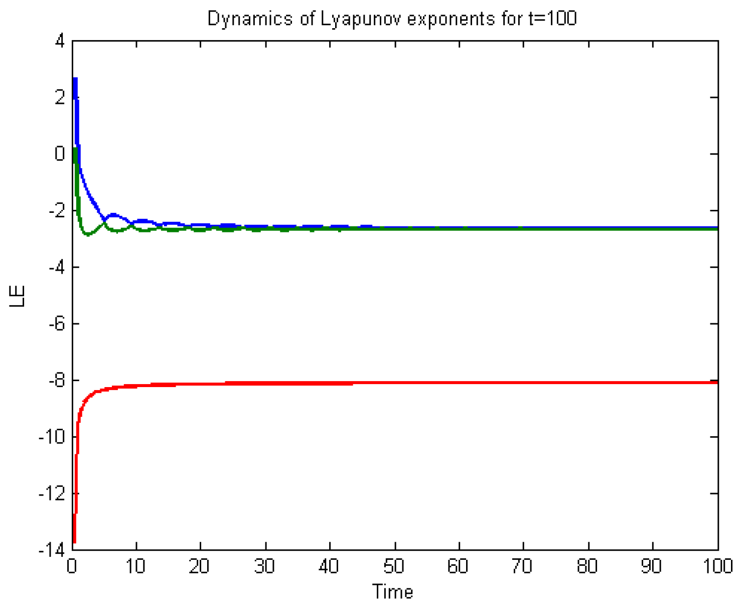
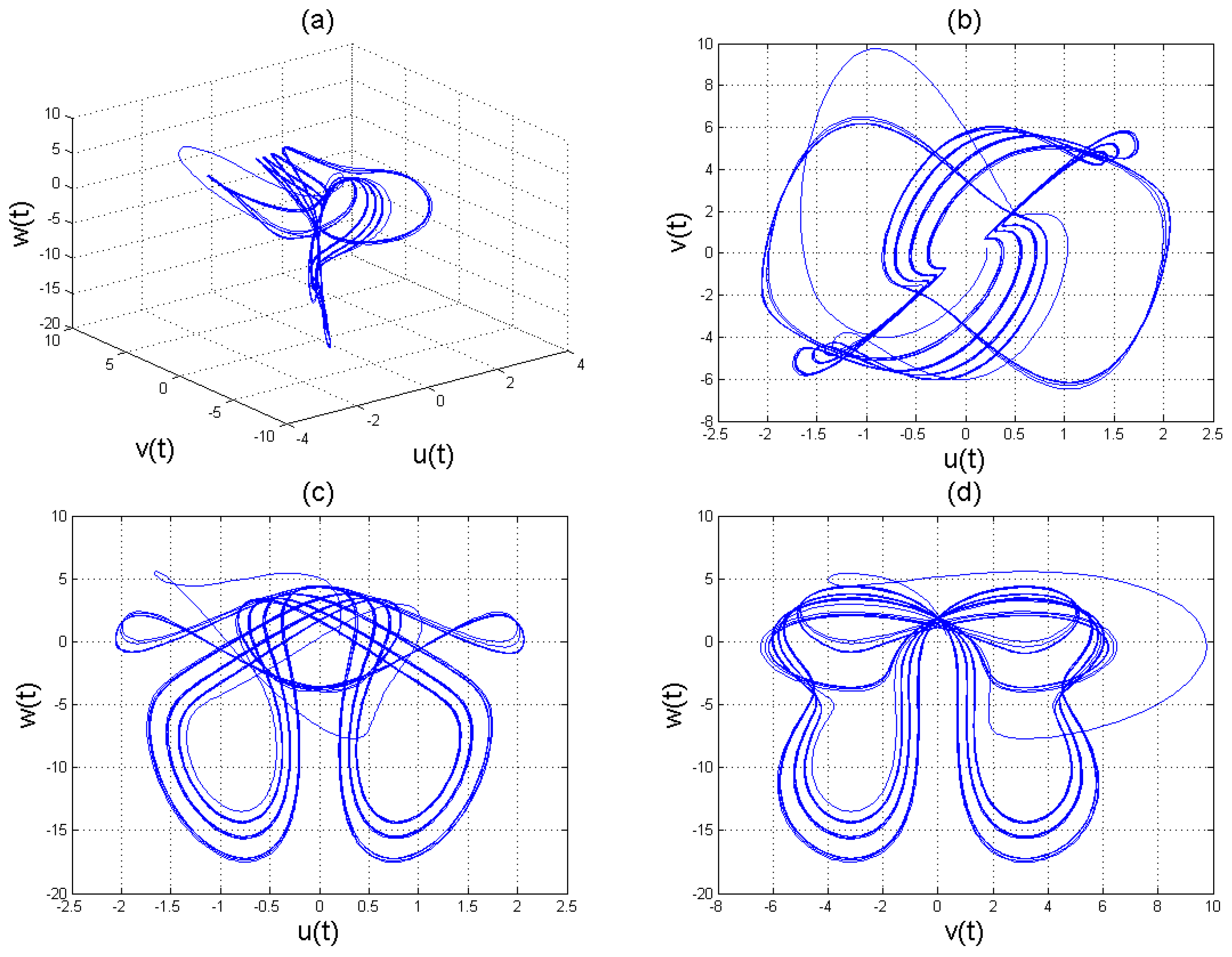
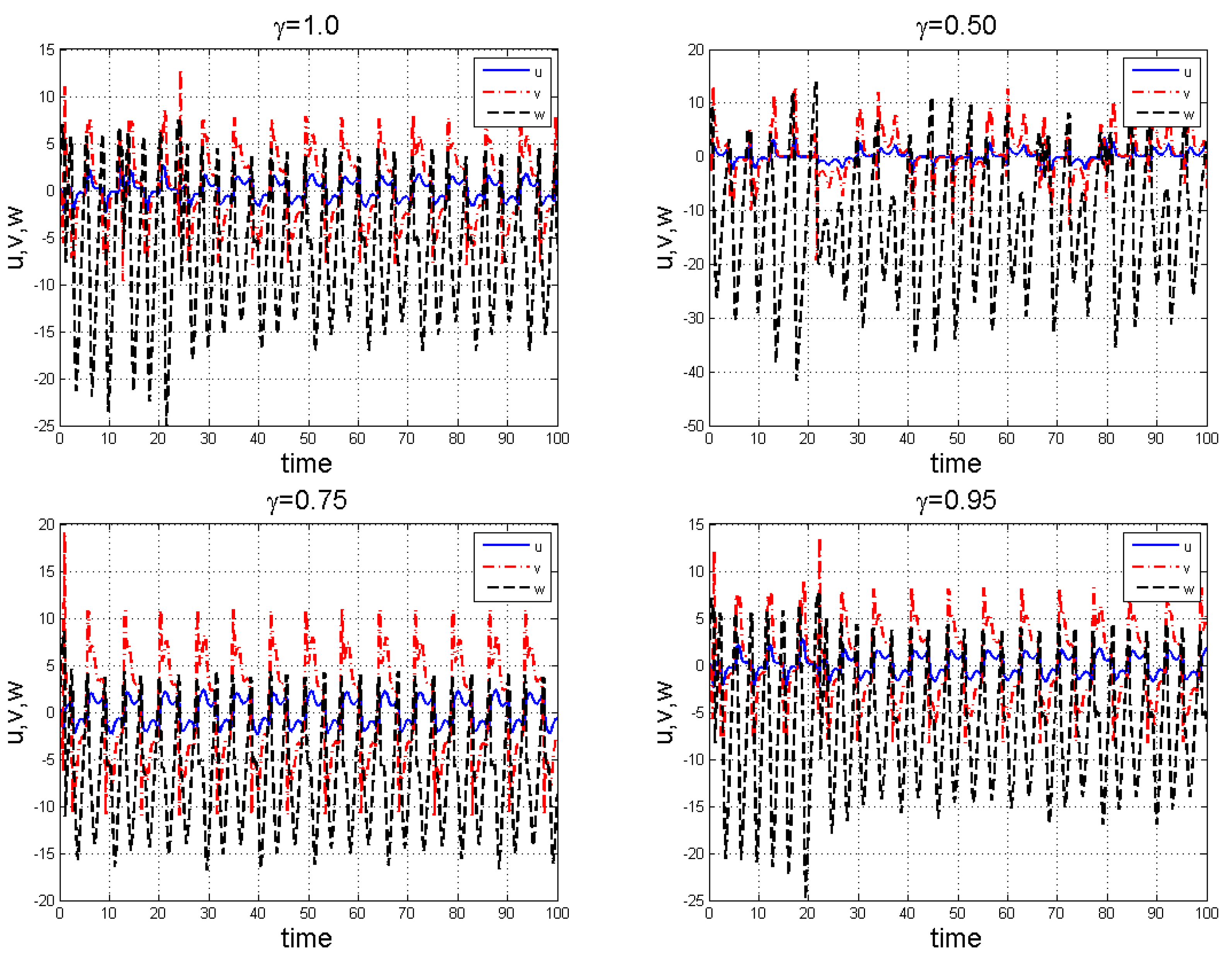
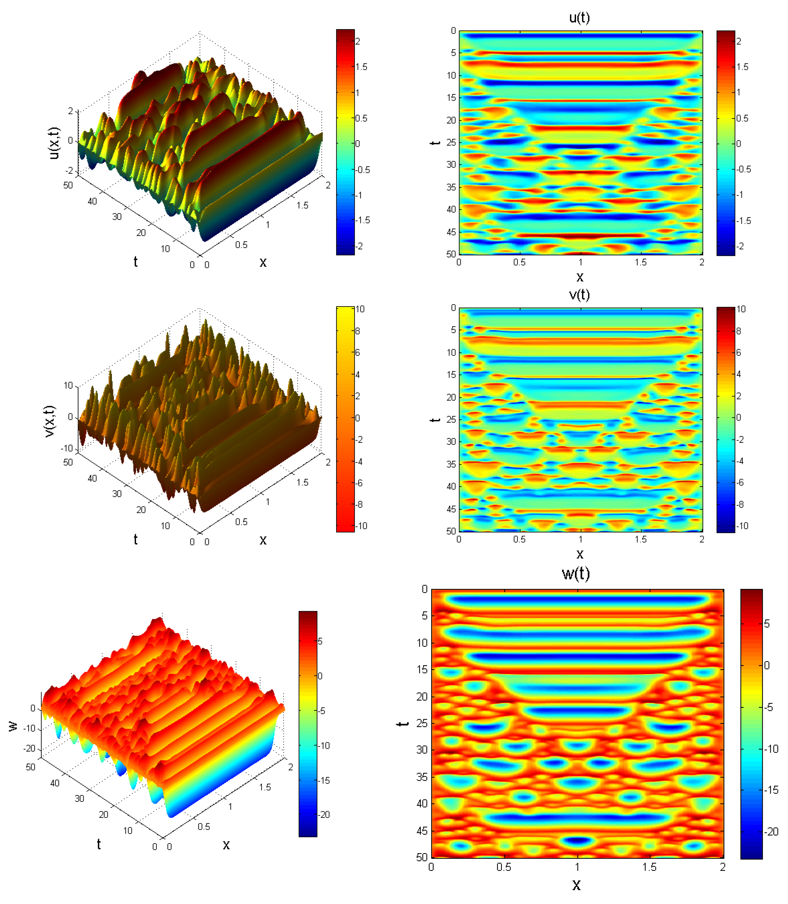
4. Experimental Results

Under this segment, we briefly report the behaviour of fractional order chaotic systems (8) and (11) governed by the influence of fractional index $\gamma$ in the sense of the Caputo operator.

In the simulation framework for system (8), we simulate with initial conditions $(u_0,v_0,w_0)=(2.6,1.8,2.5)$ and parameter values $a_1=1.8$, $a_2=0.12$, $a_3=-0.07$, and $a_4=1.5$ to obtain chaotic patterns as displayed in Figure 2, Figure 3 and Figure 4 at different instances of $\gamma$. It was observed that, regardless of the value of $\gamma$ chosen, system (8) exhibits a chaotic pattern.

For the four-scroll fractional chaotic system (11), with parameter choice:

$$\begin{array}{c}\hfill b_1=1,b_2=0.7,b_3=0.3,b_4=4,b_5=4.4,b_6=1,b_7=0.1,b_8=10,b_9=1,\end{array}$$

(22)

we observe the chaotic results as shown in Figure 5, Figure 6, Figure 7, Figure 8, Figure 9 and Figure 10 for various $\gamma$. It is clear that the chaotic pattern formation process for integer and fractional-order cases are almost similar.

In what follows, we provide an extension to system (11) to form a Caputo fractional reaction-diffusion problem as:

$$\begin{array}{ccc}\hfill {}^C{\mathcal{D}}_t^{\gamma }u& =& {\mathsf{\Delta }}^{2}u+b_{1}v-b_{2}u+b_{3}uw,\hfill \\ \hfill {}^C{\mathcal{D}}_t^{\gamma }v& =& {\mathsf{\Delta }}^{2}v-b_{4}u\left(t\right)w-b_{5}u+b_{6}vw+b_{7}u,\hfill \\ \hfill {}^C{\mathcal{D}}_t^{\gamma }w& =& {\mathsf{\Delta }}^{2}w+b_8-b_9{v}^2,\hfill \end{array}$$

(23)

where $u=u(x,t)$, $v=v(x,t)$, $w=w(x,t)$, and ${\mathsf{\Delta }}^2={\partial }^2/\partial x^2$ denotes a nonlinear Laplacian operator defined in terms of second order central finite difference operator. We choose $x\in [0,L]$ for L, which is enough for waves to propagate. System (23) is solved using the initial function set as:

$$u0=0.7\left(ones\right(N,1\left)\right),v0=1\left(ones\right(N,1\left)\right),w0=0.2\left(ones\right(N,1\left)\right),$$

(24)

so as to induce a nontrivial result. Behaviour of system (23) showing chaotic evolution is shown in Figure 11, Figure 12 and Figure 13 for different instances of fractional power $\gamma$.

5. Conclusions

A range of chaotic systems modelled by the Caputo fractional derivatives of order $\gamma$ are reported in this paper. A Chebyshev spectral method was utilised for the numerical approximation and linear mathematical analysis of the models were also considered. A number of results based on numerical simulations at some instances of fractional index were also reported with amazing chaotic patterns. It was observed that the pattern formation in integer-order systems were similar to the fractional cases.

References

1. Kilbas, A.A.; Srivastava, H.M.; Trujillo, J.J. Theory and Applications of Fractional Differential Equations; Elsevier: San Diego, CA, USA, 2006. [Google Scholar]
2. Magin, R.L. Fractional Calculus in Bioengineering; Begell House Publishers: Danbury, CT, USA, 2006. [Google Scholar]
3. Podlubny, I. Fractional Differential Equations; Academic Press: San Diego, CA, USA, 1999. [Google Scholar]
4. Ghanbari, B.; Nisar, K.S. Some Effective Numerical Techniques for Chaotic Systems Involving Fractal-Fractional Derivatives With Different Laws. Front. Phys. 2020, 1, 1–16. [Google Scholar] [CrossRef]
5. Lund, L.A.; Omar, Z.; Alharbi, S.O.; Khan, I.; Nisar, K.S. Numerical investigation of multiple solutions for caputo fractional-order-two dimensional magnetohydrodynamic unsteady flow of generalized viscous fluid over a shrinking sheet using the Adams-type predictor-corrector method. Coatings 2019, 9, 548. [Google Scholar] [CrossRef] [Green Version]
6. Pindza, E.; Owolabi, K.M. Fourier spectral method for higher order space fractional reaction-diffusion equations. Commun. Nonlinear Sci. Numer. Simul. 2016, 40, 112–128. [Google Scholar] [CrossRef] [Green Version]
7. Yildirim, A. Analytical approach to Fokker-Planck equation with space- and time-fractional derivatives by means of the homotopy perturbation method. J. King Saud Univ. Sci. 2010, 22, 257–264. [Google Scholar] [CrossRef] [Green Version]
8. Henry, B.I.; Wearne, S.L. Fractional reaction-diffusion. Physica A 2000, 276, 448–455. [Google Scholar] [CrossRef]
9. Miller, K.; Ross, B. An Introduction to the Fractional Calaulus and Fractional Differential Equations; John Wiley & Sons Inc.: New York, NY, USA, 1993. [Google Scholar]
10. Deng, J.; Ma, L. Existence and uniqueness of solutions of initial value problems for nonlinear fractional differential equations. Appl. Math. Lett. 2010, 23, 676–680. [Google Scholar] [CrossRef] [Green Version]
11. Doha, E.H.; Bhrawy, A.H.; Ezz-Eldien, S.S. A Chebyshev spectral method based on operational matrix for initial and boundary value problems of fractional order. Comput. Math. Appl. 2011, 62, 2364–2373. [Google Scholar] [CrossRef] [Green Version]
12. Khader, M.M.; Sweilam, N.H.; Mahdy, A.M.S.; Moniem, N.K.A. Numerical simulation for the fractional SIRC model and influenza A. Appl. Math. Inf. Sci. 2014, 8, 1029–1036. [Google Scholar] [CrossRef]
13. Ray, S.S.; Bera, R.K. Solution of an extraordinary differential equation by Adomian decomposition method. J. Appl. Math. 2004, 4, 331–338. [Google Scholar] [CrossRef]
14. Owolabi, K.M.; Atangana, A. Numerical simulations of chaotic and complex spatiotemporal patterns in fractional reaction-diffusion systems. Comput. Appl. Math. 2018, 37, 2166–2189. [Google Scholar] [CrossRef]
15. Owolabi, K.M.; Atangana, A. Chaotic behaviour in system of noninteger-order ordinary differential equations. Chaos Solitons Fractals 2018, 115, 362–370. [Google Scholar] [CrossRef]
16. Owolabi, K.M. Mathematical analysis and numerical simulation of chaotic noninteger order Differential systems with Riemann-Liouville derivative. Numer. Methods Partial. Differ. Equ. 2018, 34, 274–295. [Google Scholar] [CrossRef]
17. Bueno-Orovio, A.; Kay, D.; Burrage, K. Fourier spectral methods for fractional-in-space reaction-diffusion equations. BIT Numer. Math. 2014, 54, 937–954. [Google Scholar] [CrossRef]
18. Canuto, C.; Hussaini, M.Y.; Quarteroni, A.; Zang, T.A. Spectral Methods in Fluid Dynamics; Springer: New York, NY, USA, 1988. [Google Scholar]
19. Kosmatov, N. Integral equations and initial value problems for nonlinear differential equations of fractional order. Nonlinear Anal. 2009, 70, 2521–2529. [Google Scholar] [CrossRef]
20. Snyder, M.A. Chebyshev Methods in Numerical Approximations; Prentice-Hall: Upper Saddle River, NJ, USA, 1966. [Google Scholar]
21. Akgul, A.; Moroz, I.; Pehlivan, I.; Vaidyanathan, S. A new four-scroll chaotic attractor and its engineering applications. Optik 2016, 127, 5491–5499. [Google Scholar] [CrossRef]
22. Behinfaraz, R.; Ghaemi, S.; Khanmohammadi, S. Adaptive synchronization of new fractional-order chaotic systems with fractional adaption laws based on risk analysis. Math. Meth. Appl Sci. 2019, 42, 1772–1785. [Google Scholar] [CrossRef]
23. Akgul, A.; Hussain, S.; Pehlivan, I. A new three-dimensional chaotic system, its dynamicalanalysis and electronic circuit applications. Optik 2016, 127, 7062–7071. [Google Scholar] [CrossRef]
Figure 1. Dynamic of the Lyapunov exponent for system (8).
Entropy 22 01027 g001
Figure 2. Chaotic evolution of fractional system (8) at γ = 0.38 . Plots (a) 3D chaotic attractor, (bd) are 2D chaotic distributions, and (e) chaotic time-series solution.
Entropy 22 01027 g002
Figure 3. Chaotic evolution of fractional system (8) at γ = 0.51 . Plots (a) 3D chaotic attractor, (bd) are 2D chaotic distributions, and (e) chaotic time-series solution.
Entropy 22 01027 g003
Figure 4. Chaotic evolution of fractional system (8) at γ = 0.99 . Plots (a) 3D chaotic attractor, (bd) are 2D chaotic distributions, and (e) chaotic time-series solution.
Entropy 22 01027 g004
Figure 5. Chaotic attractors involving the Caputo fractional order derivative for the four-scroll chaotic system (11) with γ = 1 .
Entropy 22 01027 g005
Figure 6. Chaotic attractors involving the Caputo fractional order derivative for the four-scroll chaotic system (11) with γ = 0.38 .
Entropy 22 01027 g006
Figure 7. Chaotic attractors involving the Caputo fractional order derivative for the four-scroll chaotic system (11) with γ = 0.50 .
Entropy 22 01027 g007
Figure 8. Chaotic attractors involving the Caputo fractional order derivative for the four-scroll chaotic system (11) with γ = 0.61 .
Entropy 22 01027 g008
Figure 9. Chaotic attractors involving the Caputo fractional order derivative for the four-scroll chaotic system (11) with γ = 0.84 .
Entropy 22 01027 g009
Figure 10. Time series showing chaotic evolution of system (11) for several values of γ .
Entropy 22 01027 g010
Figure 11. Evolution of system (23) at γ = 0.50 , x [ 0 , 2 ] for t = 50 Chaotic behaviour is noticeable.
Entropy 22 01027 g011
Figure 12. Evolution of system (23) at γ = 0.67 , x [ 0 , 2 ] for t = 50 . Chaotic distribution is noticeable.
Entropy 22 01027 g012
Figure 13. Evolution of system (23) at γ = 0.99 , x [ 0 , 5 ] for t = 5 . Chaotic behaviour is evident.
Entropy 22 01027 g013