2.1. Quantum State Fidelity Estimation Employing State Verifiers
In a quantum information processing employing a pure state
in a bipartite
d-dimensional system
, the very first task is to create bipartite quantum states as close as possible to the target state
. To evaluate how good a state preparation is, one can estimate the
-state fidelity
of the generated states
in local measurements, where the state fidelity
is defined as
In this section, we review the strategy operators employed in QSV [
20,
21,
22,
23,
24], and their application in QSFE. In QSFE, one evaluates expectation values of certain observables from the whole measurement outputs instead of testing each input by each output of measurements according to a “strategy”; we therefore refer to the “strategy” in QSV as “state verifier operators” in the context of QSFE in this paper.
In the measurement of the computational basis
, one can verify the testing state
by the characteristic correlations of the target state
. The probability of the outputs satisfying the target characteristic correlations is determined to the expectation value of the following
-state stabilizer:
We call a stabilizer of the target state a -state verifier. If the measurement in the Schmidt basis of is feasible and efficient in a laboratory, it is preferable to choose the Schmidt basis as the computational basis, since the state verifier constructed in the Schmidt basis has the least rank, which means that can detect the -orthogonal part of a testing state more efficiently.
To estimate the quantum state fidelity, a single state verifier in the computational basis is not enough, since
is not the only one state that is stabilized by
. To construct a state verifier that stabilizes only the target state
, one needs to include the state verifiers in the other measurement basis. Let
a set of measurement configurations additional to the computational basis
where
are POVM measurements in the
d-dimensional local system
. The POVM measurements
are constructed with
measurement operators
, which are projections onto the corresponding measurement-basis states
,
Note that, for projective measurements with orthogonal basis states, there is no need to add the factor
in Equation (
4). However, for consistency of formulation, we adopt the representation in Equation (
4) for projective measurements. In each measurement configuration
, one can construct a state verifier operator
by adding up its corresponding measurement operators
with weights
, such that
stabilizes the target state.
Lemma 1 (Construction of a state verifier in local POVM measurements)
. The state verifier in the measurement configuration that stabilizes can be explicitly constructed byHere, the weights are determined by a transformation operator that maps the local computational basis states to the measurement basis states associated with the local POVM as follows: A good measurement configuration
should have nonzero
in its state verifier
as few as possible, which leads to the minimum rank of
and better detection efficiency of
-orthogonal states. For this reason, POVM measurements are preferable for most bipartite states in general. For example, for the general Bell-type states that will be studied in
Section 2.3, the POVM measurements that are associated with the generalized Heisenberg–Weyl operators defined in Equation (
24) lead to the state verifiers derived in Equation (
29), which have the minimum rank of
d. For the maximally entangled states, the projective measurements in the mutually unbiased bases are the optimum configurations. In this case, the state verifiers
are local unitary transformations of
.
By mixing the state verifiers
that are associated with the measurement settings in
, one can construct a state verifier
,
Together with the state verifier
in the computational basis, one can then construct a
-state verifier operator, which only stabilizes the target state
,
Since the
-state verifier
is a Hermitian stabilizer of
by definition, the
-state verifier can be decomposed into the mixture of the projection onto the target state and its orthogonal part
, i.e.,
with
. Note that the state verifier
is called a verification strategy in the context of quantum state verification (QSV). Let
be the eigenvalues of the
-orthogonal operator
associated with the eigenstates
. The maximum and minimum eigenvalue
of
determines the efficiency of the verification strategy in QSV as well as the fidelity bounds in QSFE [
23],
Let
and
be the eigenstates of
associated with the maximum and minimum eigenvalues
and
, respectively. The lower bound in Equation (
9) can be achieved by the testing states
in the Hilbert subspace that is spanned by the target state
and the maximum-eigenvalue state
, while the upper bound can be achieved by the states
. However, the noises in a state generation process are in general not the eigenstates
or
of the operator
, which means that the bounds in Equation (
9) are not the tightest for a particular noisy state generation. As the fidelity lower bound can be employed for entanglement dimensionality certification [
19], a tighter fidelity lower bound in a state fidelity estimation implies the better robustness of the entanglement detection against the noises that present in the experiment. It is therefore desirable to refine the fidelity bounds in QSFE by adapting the estimation approach to the noises of a particular state generation.
2.2. Quantum State Fidelity Estimation Assisted with Measurement Statistics in the Computational Basis
In this section, we employ the state verifiers in a scenario of quantum state fidelity estimation under the assumption that the computational-basis measurement is more efficient and feasible than the other measurement configurations. In this case, one can first measure a testing state
in the computational basis and obtain the corresponding measurement statistics:
This measurement statistics contains information about the noises in a state generation. These noises can contribute to the expectation value of the
-orthogonal part
of the state verifier
,
where
and
are the
-orthogonal part of
and
, respectively,
To estimate the state fidelity
, one will need to exclude the contribution of
-orthogonal part
from the expectation value of the state verifier
, since
. In Equation (
9), the expectation value
is bounded by its maximum and minimum eigenvalues,
which does not depend on the measurement statistics
. Here, the a priori information of the computational-basis measurement statistics
can help us to adjust the measurement configurations
to the noises of the systems and refine the bounds on the expectation value
.
To estimate
exploiting the measurement statistics
, one can bound the operator
by an operator
, which is diagonal in the computational basis,
where
is the non-zero diagonal part of the
-orthogonal operator
assigned by a weight
,
The operator
contains the information of the
-orthogonal contributions in
, which are the errors that we want to exclude from the state verifier. This information can be extracted from the measurement statistics
in the computational basis by the operator
prior to the implementation of the measurement
. It can help us to evaluate the measurement configurations
and to bound the operator
exploiting the a priori statistics
. The operator
can be decomposed into the
projector and a non-
component
,
The expectation value
is the sum of the state fidelity
and the expectation value
, which contains partial information about the
-orthogonal contribution
of a testing state in the expectation value of the state verifier
. One can show that there exists an assignment of the weights
in
, such that the operators
and
can be decomposed by a set of pure state
,
where
are in general non-orthogonal,
are non-negative and
are positive. One can then bound the operator
by
with two real-value coefficients
and
such that
, which refines the bounds on the
-orthogonal contribution
in
given in Equation (
13),
As a result, one can then refine the bounds on the state fidelity given in Equation (
9) as follows.
Lemma 2 (Bounds on state fidelity)
. The state fidelity for a target state is bounded bywhere α and β are the maximum and minimum ratio between and A trivial construction of
is the assignment of
, which leads to
. For this construction, the decomposition in Equation (
17) is the eigenstate decomposition of
. In this case, the bounds in Equation (
19) coincide with the bounds given in Equation (
9). Since
is constant and does not depend on the measurement configurations
and measurement statistics
in the computational basis, it can not be employed to adapt the measurement configurations
to
.
In order to adapt the measurement configurations
to
, one needs to introduce the
and
dependency in
, such that one can find the optimal measurement configuration
for the minimum
subject to a given measurement statistics
. To this end, one can explicitly construct a nontrivial
and determine the coefficients
following the protocol given in the proof of Lemma 2 in
Section 4 (Methods). Employing the operator
constructed in Equation (
55), one can then adapt the measurement configurations
to the measurement statistics
such that the expectation value
is minimum subject to a given
, which leads to a higher lower bound on the state fidelity. Usually, the coefficient
is zero, unless one chooses a large set of measurement configurations such that the state verifier
has the same rank as
. As a consequence, the minimization of
does not affect the upper bound in most cases. Following these steps, one can therefore construct the subsequential measurements
depending on the measurement statistics in the computational basis
, which means the operators
and
in Equation (
19) also depend on
,
As a result, Lemma 2 allows us to estimate quantum state fidelity employing
and
adapted to the measurement statistics in the computational basis
to obtain tighter bounds. In the next section, we will employ this method to derive an adaptive approach of quantum state fidelity estimation for Bell-type states explicitly.
2.3. Adaptive State Fidelity Estimation for Bell-Type States
A general Bell-type entangled state in
Hilbert state is an entangled state with the Schmidt rank
d, which is an important higher dimensional entanglement resource in bipartite systems. If the Schmidt basis happens to be more feasible than the other basis in a laboratory, one can employ the Schmidt basis as the computational basis in our adaptive estimation approach. In this case, a bipartite pure state is decomposed as
where
are the Schmidt coefficients. In order to construct a state verifier for a Bell-type state
, one needs to construct stabilizers of
employing measurement operators in different measurement bases. In the computational basis, the state verifier
that characterizes the correlations of the target state
is given by
For the construction of state verifiers in the other measurement bases, one needs the other stabilizers of the Bell-type state
, which can be derived from the standard Heisenberg–Weyl (HW) operators [
25] with a modification associated with a coefficient vector
. A
-modified HW operator
is comprised of the
-modified shift operator
and the clock operator
,
where the
-modified shift operator
and the clock operator
are defined as
with
and
. Here, the symbol “⊕” stands for the
d-modulus plus ( The symbol
(
) is employed to denote the
d-modulus plus (minus) of two quantities, e.g.,
and
. For conciseness, we omit the subscript
d.). Note that the relevant HW operators in this paper are the operators with the label
, of which the notation are simplified by
. The target Bell-type state
is stabilized by all the local HW operators
with the modification coefficients
satisfying
As a consequence, the measurement configurations
for the
-state verifier can be constructed in the eigenbasis of the
-modified HW operators,
where the local POVM measurement
in the
eigenbasis
consists of the measurement operators
as defined in Equation (
4). To implement such a measurement, one has to know the explicit form of the
eigenstates
in the computational basis, which are constructed by
As one can show that
by simply applying
on the state, the eigenstate
is associated with the eigenvalue
. Since the eigenstate
depends on the coefficient
, the set of measurement configurations
are therefore determined by the coefficients
, which can be adapted to the measurement statistics
in the computational basis, i.e.,
. In each measurement configuration
, one can construct its corresponding state verifier
according to Lemma 1,
The state verifier
has the minimum rank of
d, which is optimum for a Bell-type state
in a
-dimensional Hilbert space. The state verifier
associated with the non-computational-basis measurement configurations
is then comprised of
with certain weights
according to Equation (
7).
Together with the state verifier
in the computational basis, one can construct a
-state verifier
according to Equation (
8). To estimate the state fidelity, one still needs to construct the operator
, where the error operator
can be determined according to Equation (
55) as follows:
The error operator
characterizes the unexpected outputs for the target state
in the computation basis, which still contribute to the expectation value of the state verifier
in the subsequential measurements
. Employing the operators
and
, one can then estimate the lower and upper bounds on the
-state fidelity
according to Lemma 2.
In a laboratory, there will be a set of available measurement configurations
. However, taking all the available measurement configurations into the construction of the state verifier
does not always give us better bounds on the state fidelity. Let
be the prime number factorization of the local dimensionality
d with
. One can show that the optimum bound on the state fidelity
determined by Lemma 2 is achieved by the subsets
of
, which are constructed by selecting one element from each
-modulus equivalent subclass (quotient subset)
of
. Here, a
-modulus subclass
of
is defined as
From each nonempty subclass
, one selects a measurement configuration to construct a subset
of the available measurement configurations
. The set of all possible measurement configurations under this construction is
The cardinality of the subset of measurement configurations
is equal to the number of nonempty
-modulus subclasses
of
, which is denoted by
. We can then assign a state verifier
to each measurement configuration subset
according to Equation (
7) to determine a lower bound on
. One can show that the optimum choice of the weights
for
in
is the uniform weight
, which takes the average of the state verifiers
in
As a result of Lemma 2, one can estimate the lower and upper bounds on the
-state fidelity as follows.
Theorem 1 (Lower and upper bounds on the state fidelity)
. Let be a set of measurement configurations associated with the local POVM measurements , which are available in a laboratory. The state fidelity is then lower bounded byIf d is prime and , the value of can be explicitly determined by For a prime dimension
d, the lower and upper bounds on the state fidelity for the Bell-type state
in Equation (
19) coincide with each other, which leads to an exact value of the state fidelity given in Equation (
36). One can therefore directly measure a state fidelity in
measurement configurations. In this case, the method of state fidelity estimation in Equation (
36) is equivalent to the state fidelity derived in [
19]. Since the state fidelity is exactly measured, the choices of the coefficients
do not affect the final result ( Theoretically, the exact value of the
-state fidelity of a testing state should not depend on the measurement configurations, if one has large enough data of measurement outputs.). One can therefore choose
according to the feasibility of their corresponding measurement settings. Note that the most simple measurement is usually the projective measurement with the uniform coefficient
. As a result of Equation (
26), the preferable measurement settings in this case are then the projective measurements associated with
on one local system
A combined with the POVM measurements associated with
on the other local system
B.
If
d is non-prime or
, there will be a gap between the lower and upper bounds on the state fidelity given in Equations (
34) and (
35). This gap can be reduced by carefully choosing proper coefficients
adapted to the measurement statistics in the computational basis before the implementation of remaining measurement configurations
. Since the only information we have is the measurement statistics in the computational basis, we can not optimize
for the maximum expectation value of the state verifier
that is evaluated in the upcoming measurements. The optimization that we can carry out at this stage is to find the optimum
for the minimum expectation value of the error operator
as follows:
The following conditions are sufficient for the minimum expectation value
However, these conditions can not be fulfilled for all
in general. For the special case when the measurement statistics is approximately symmetric under the exchange of the local systems, i.e.,
, the expectation value of the error operator is lower bounded by
where the minimum is achieved by
In practice, one may just want to estimate the state fidelity for the Bell-type state that is closest to the testing state, rather than a predefined one. In this case, one can even adapt the Schmidt coefficients
to the measurement probability
such that
As a whole, one can estimate a lower and an upper bound on the state fidelity for the Bell-type state that is closest to a testing state adaptively in the following steps:
One implements a measurement in the computational basis to obtain the statistics .
Adapted to the measurement statistics
, one finds the optimum coefficients
for the minimum expectation value of the error operator
according to Equation (
37).
Depending on the facilities of a laboratory, one implements a set of available local POVM measurements
associated with the
-modified Heisenberg–Weyl operators
according to Equations (
27) and (
28).
From the measurement statistic obtained in each measurement configuration , one evaluates the corresponding state verifier operator .
Employing Theorem 1, one estimates a lower and an upper bound on the state fidelity .
2.4. Adaptive State Fidelity Estimation in Noisy Bell-Type State Preparation
In this section, we demonstrate the fidelity estimation method derived in Theorem 1 for Bell-type quantum states prepared under certain types of noises. As an example, we first consider the white noises, which are symmetric under the exchange of two local systems. In entanglement generation of a Bell-type state with the white noises, the final state is described by
where
is the weight of the white noises. The measurement statistics in the computational basis
is symmetric under the exchange of the local systems
. One can therefore choose the measurement coefficients
as given in Equation (
40). In this case, our approach employs the same measurement configurations as the ones employed in [
19]. If one just exploits one measurement configuration added to the computational basis, the lower bound derived in [
19] is tighter than the bound in Theorem 1. However, as the number of measurement configurations in
increases, the lower bound in Theorem 1 is improved faster, and becomes better than the one derived in [
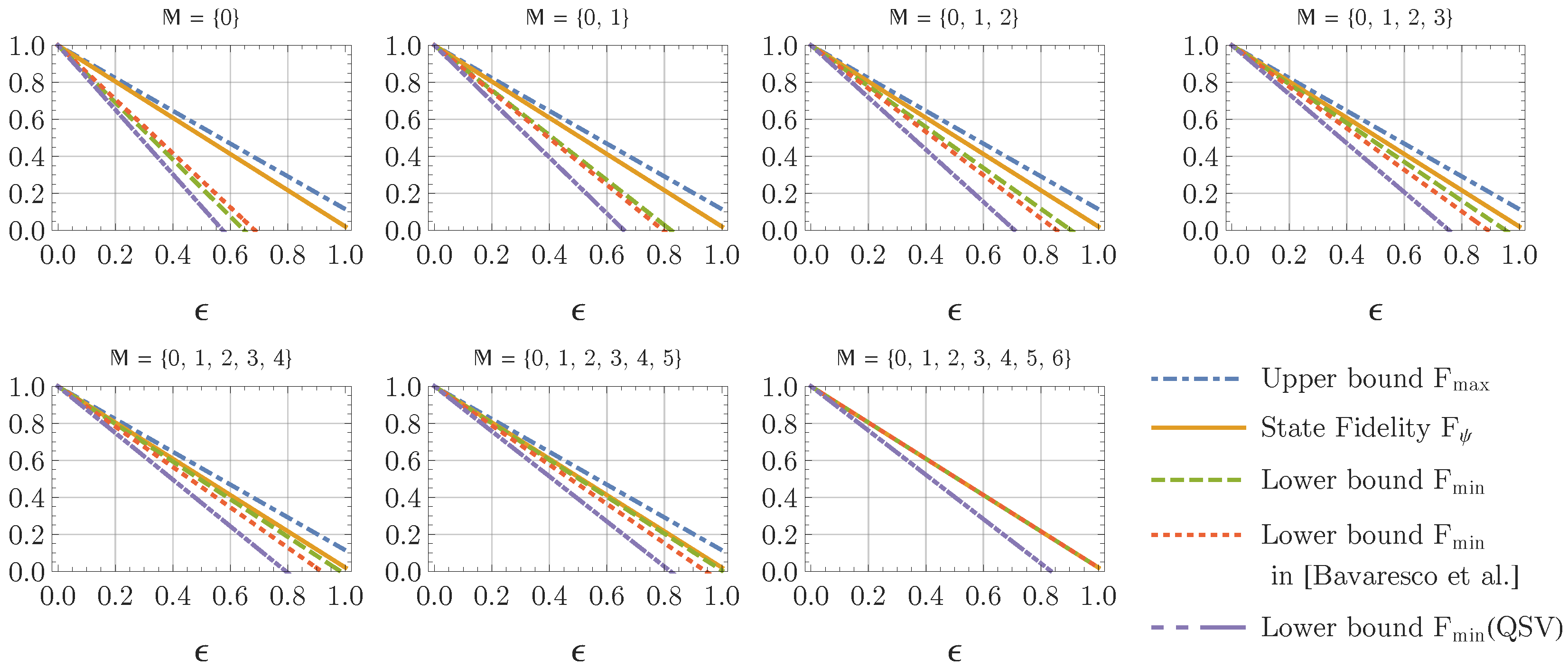
19], which can be seen from the comparison between these two bounds in
Figure 1 for a prime dimension
.
In
Figure 1, we plot the state fidelity
(orange solid) of a
-dimensional testing state
, and its corresponding upper (blue dot-dashed) and lower (green dashed) bounds determined by Theorem 1. These lower bounds are compared with the lower bounds derived in [
19] (red dotted) and the ones obtained by the nonadaptive method in Equation (
9) (violet dot-dot-dashed). From this example, one can see that the lower bounds derived in Theorem 1 become tighter than the one in [
19], if one chooses more than one measurement configurations
. One can also see that both the adaptive methods in Theorem 1 and in [
19] can determine tighter lower bounds than the nonadaptive method in Equation (
9).
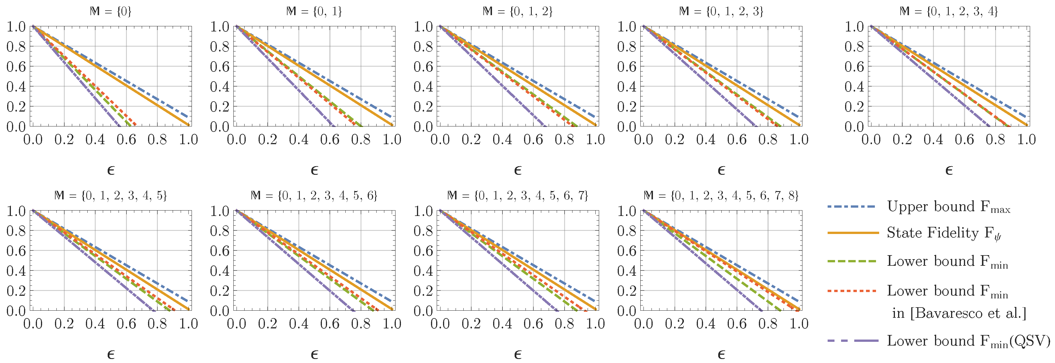
A limitation of the fidelity estimation in Theorem 1 is that, for a non-prime dimension, the lower bounds are not necessarily tighter, if the number of measurement configurations increases. According to Theorem 1, if the available measurement configurations
have more than
settings, then one should take the maximum of the lower bounds estimated by all subsets
of
, which has one element in each
-modulus subclass. In this case, the optimum lower bound obtained in Theorem 1 can be already saturated, when
. As one can observe in
Figure 2 for
, the optimum lower bounds on
derived in Theorem 1 are already achieved by
, while the lower bounds derived in [
19] are continuously improved, as one includes more measurement configurations. When one includes enough measurement configurations such that
, the method in [
19] can provide tighter lower bounds than the ones derived in Theorem 1, while for the measurement configurations
, the method in Theorem 1 is still better.
In general, the noises in two separated local systems
are not symmetric under the exchange of local systems. In this case, Theorem 1 allows us to adapt the measurement coefficients
to the measurement statistics in the computational basis to refine the state fidelity estimation. For example, in linear optics networks [
26] which have path modes as their degree of freedom, one possible type of error is crosstalk between the computational basis states associated with neighboring paths. If the crosstalk error is small enough, such that the crosstalk between the computational-basis states
and
associated with far neighboring paths
is negligible relative to the crosstalk between the closest neighboring paths
, i.e.,
for
, the expectation value
can be approximately given by
In this case, the optimum
determined by Equations (
38) and (
41) can be solved by
where
are the normalization factors. As an example, a state produced in a Bell-type state generation under a simple model of local cross-talking noises
can be described by
Here, the error coefficients
and
are the probability of a photon crossing to a closest neighboring path in the local system
A and
B, respectively. According to Equation (
44), the optimum
for one-side cross-talking errors are
For symmetric cross-talking errors
, the probability distribution
is symmetric under the exchange of
A and
B, the minimum of
is then achieved by the measurement coefficients
The computational-basis measurement statistics of the testing states
and
with one-side local crosstalk is asymmetric (see
Figure 3a,c), while it is symmetric for the testing state
with symmetric cross-talking errors (see
Figure 3b). The lower bounds obtained by the different choices of measurement coefficients
given in Equations (
46) and (
47) are compared in
Figure 3d, where we fix the total cross-talking probability by
and calculate the fidelity lower bounds for different values of the ratio
. One can observe a
improvement on the lower bound estimation, if one chooses the optimum coefficients
in Equation (
44), rather than the symmetric coefficients in Equation (
47) for the one-side cross-talking errors
and
.


