A Simple Model to Relate the Elastic Ratio Gamma of a Critically Self-Organized Spring-Block Model with the Age of a Lithospheric Downgoing Plate in a Subduction Zone

 , ,
, ,
Abstract
1. Introduction
2. A Simple Model to Relate the OFC Elastic Ratio γ with the Age of the Lithospheric Downgoing Plate
3. A Simple Model to Relate the OFC Elastic Ratio γ with the Age of the Lithospheric Downgoing Plate
4. Extended Ruff–Kanamori Diagram
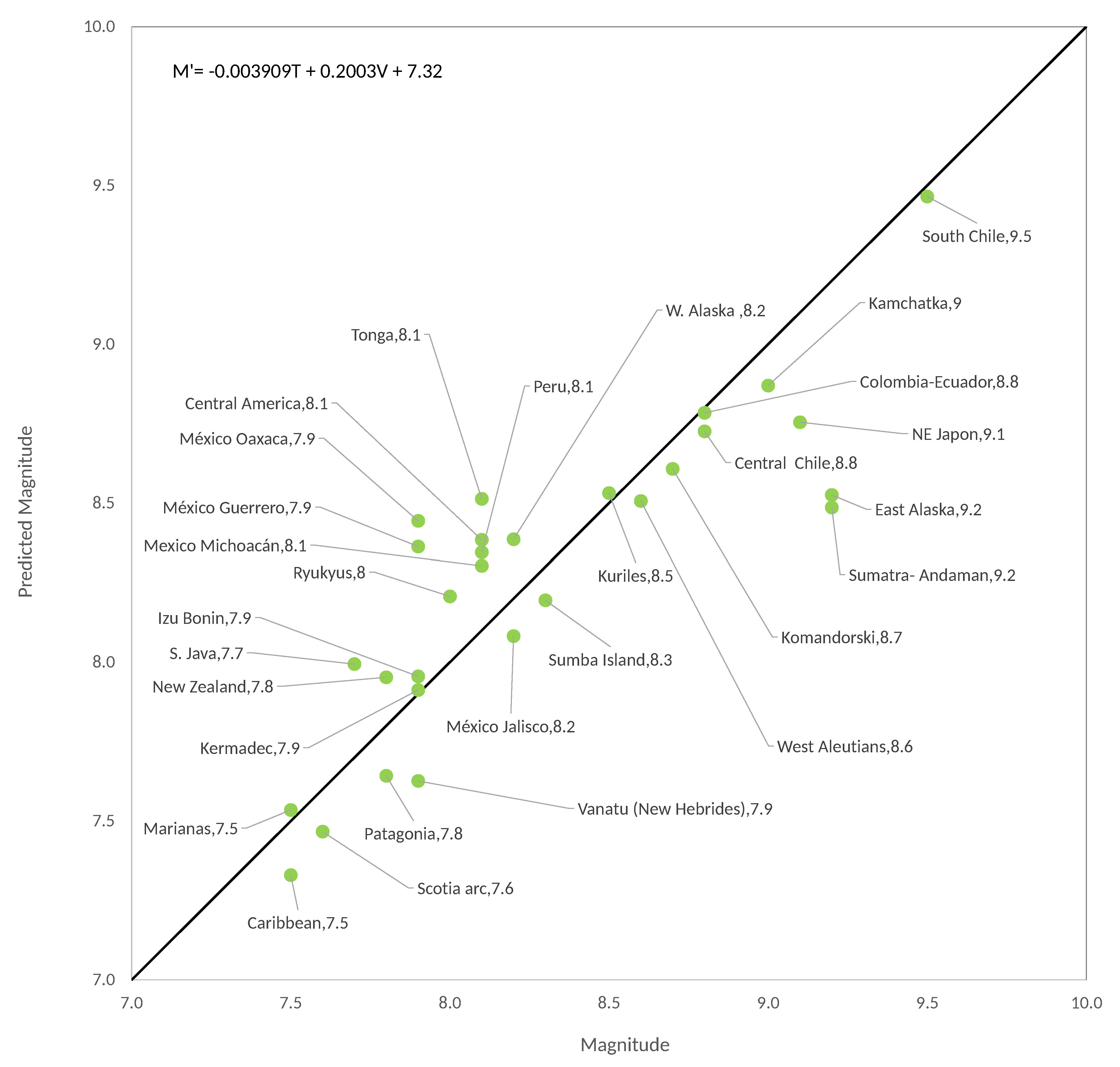
4.1. Real Seismicity
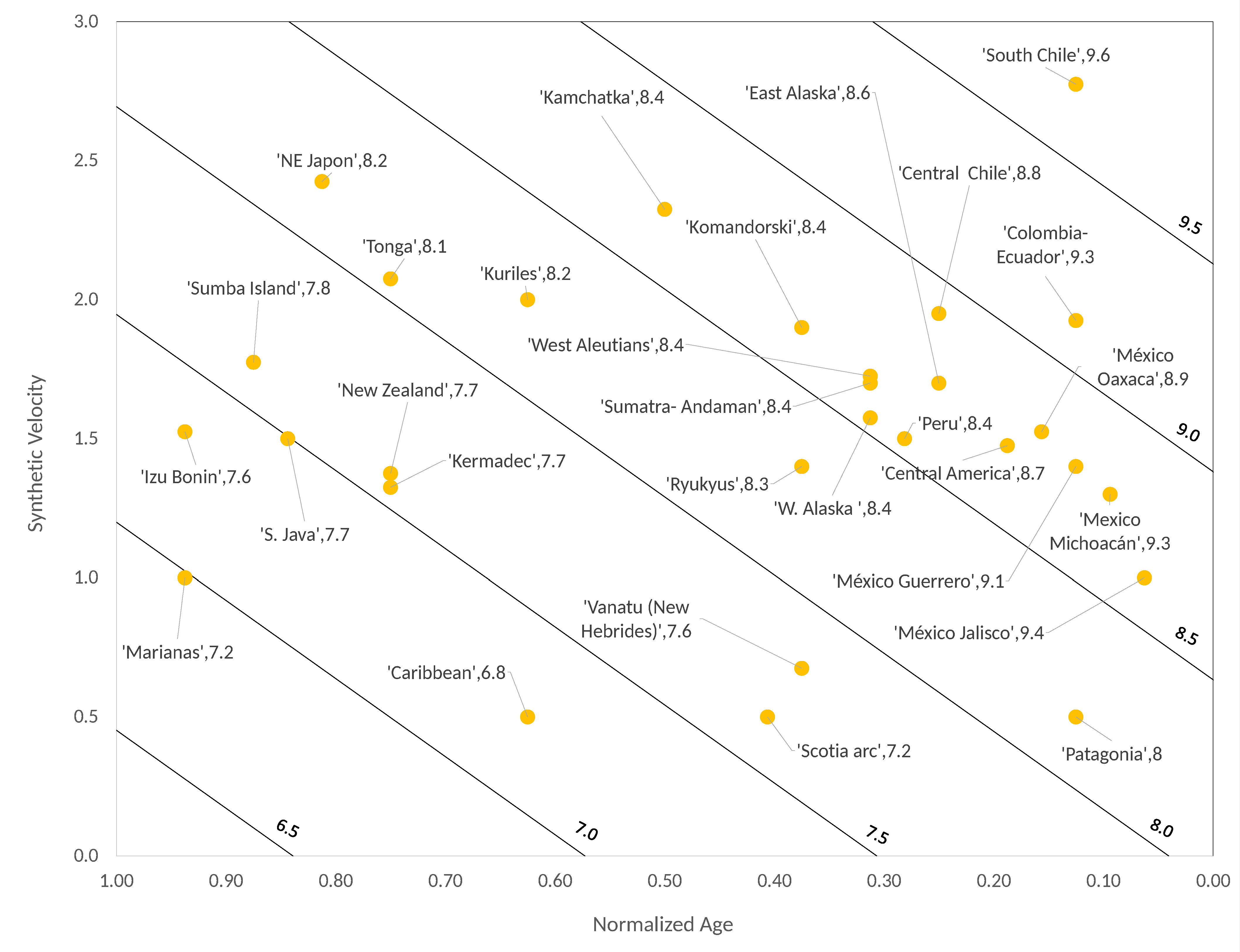
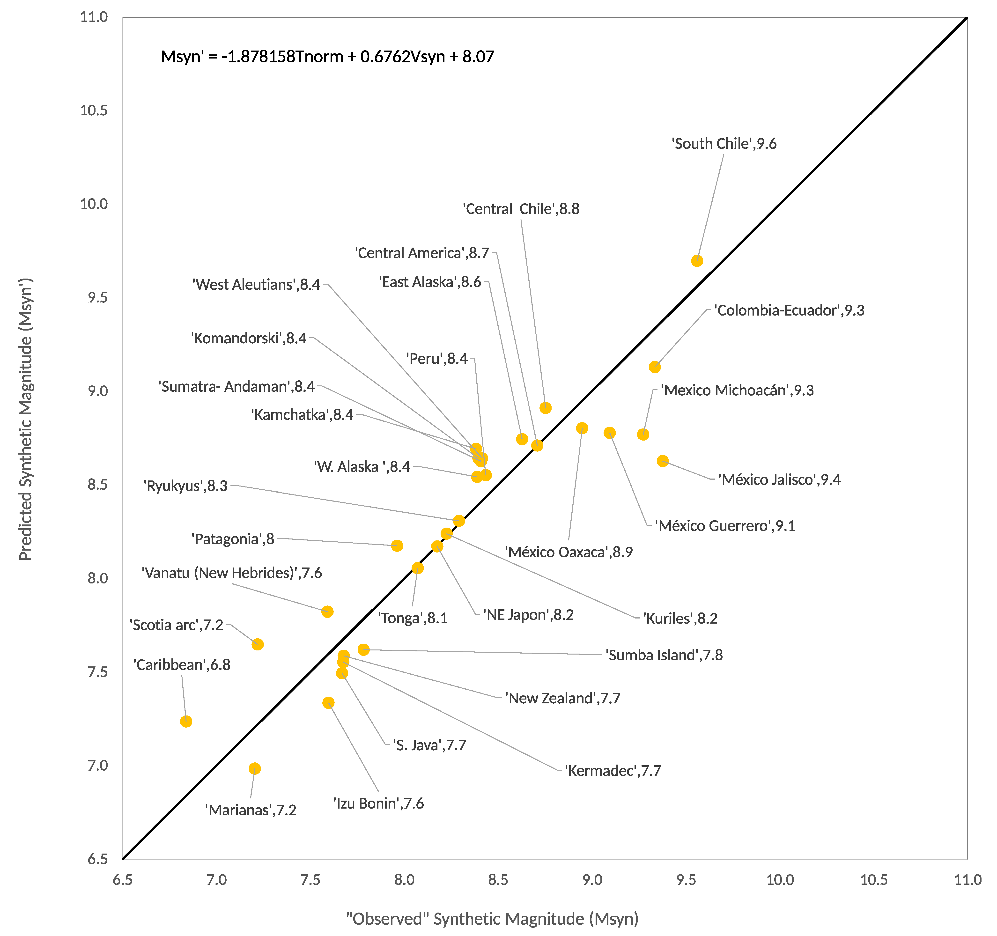
4.2. Synthetic Seismicity
5. Discussion
6. Conclusions
Author Contributions
Funding
Acknowledgments
Conflicts of Interest
References
- Kanamori, H. Rupture process of subduction-zone earthquakes. Annu. Rev. Earth Planet. Sci. 1986, 14, 293–322. [Google Scholar] [CrossRef]
- Uyeda, S.; Kanamori, H. Back-arc opening and the mode of subduction. J. Geophys. Res. Solid Earth 1979, 84, 1049–1061. [Google Scholar] [CrossRef]
- Ruff, L.; Kanamori, H. Seismicity and the subduction process. Phys. Earth Planetary Inter. 1980, 23, 240–252. [Google Scholar] [CrossRef]
- Scholz, C.H. The Mechanics of Earthquakes and Faulting; Cambridge University Press: Cambridge, UK, 2018. [Google Scholar] [CrossRef]
- Bak, P.; Tang, C. Earthquakes as a Self-Organized Critical Phenomenon. J. Geophys. Res. 1989, B94, 15635. [Google Scholar] [CrossRef]
- Sornette, A.; Sornette, D. Self-organized criticality and earthquakes. EPL (Europhys. Lett.) 1989, 9, 197. [Google Scholar] [CrossRef]
- Ito, K.; Matsuzaki, M. Earthquakes as self-organized critical phenomena. J. Geophys. Res. Solid Earth 1990, 95, 6853–6860. [Google Scholar] [CrossRef]
- Chen, K.; Bak, P.; Obukhov, S.P. Self-organized criticality in a crack-propagation model of earthquakes. Phys. Rev. A 1991, 43, 625. [Google Scholar] [CrossRef]
- Brown, S.R.; Scholz, C.H.; Rundle, J.B. A simplified spring-block model of earthquakes. Geophys. Res. Lett. 1991, 18, 215–218. [Google Scholar] [CrossRef]
- Olami, Z.; Feder, H.J.S.; Christensen, K. Self-organized criticality in a continuous, nonconservative cellular automaton modeling earthquakes. Phys. Rev. Lett. 1992, 68, 1244. [Google Scholar] [CrossRef]
- Watkins, N.W.; Pruessner, G.; Chapman, S.C.; Crosby, N.B.; Jensen, H.J. 25 Years of Self-organized Criticality: Concepts and Controversies. Space Sci. Rev. 2016, 198, 3–44. [Google Scholar] [CrossRef]
- Perez-Oregon, J.; Muñoz-Diosdado, A.; Rudolf-Navarro, A.H.; Guzmán-Sáenz, A.; Angulo-Brown, F. On the possible correlation between the Gutenberg-Richter parameters of the frequency-magnitude relationship. J. Seismol. 2018, 22, 1025–1035. [Google Scholar] [CrossRef]
- Perez-Oregon, J.; Muñoz-Diosdado, A.; Rudolf-Navarro, A.H.; Angulo-Brown, F. Some common features between a spring-block self-organized critical model, stick-slip experiments with sandpapers and actual seismicity. Pure Appl. Geophys. 2019. [Google Scholar] [CrossRef]
- Angulo-Brown, F.; Muñoz-Diosdado, A. Further seismic properties of a spring-block earthquake model. Geophys. J. Int. 1999, 139, 410–418. [Google Scholar] [CrossRef]
- Gutenberg, B.; Richter, C.F. Frequency of earthquakes in California. Bull. Seismol. Soc. Am. 1944, 34, 185–188. [Google Scholar]
- Geller, R.J.; Jackson, D.D.; Kagan, Y.Y.; Mulargia, F. Earthquakes cannot be predicted. Science 1997, 275, 1616. [Google Scholar] [CrossRef]
- Heuret, A.; Lallemand, S.; Funiciello, F.; Piromallo, C.; Faccenna, C. Physical characteristics of subduction interface type seismogenic zones revisited. Geochem. Geophys. Geosyst. 2011, 12, Q01004. [Google Scholar] [CrossRef]
- Montgomery, D.C.; Runger, G.C.; Hubele, N.F. Engineering Statistics, 5th ed.; Wiley: Hoboken, NJ, USA, 2011. [Google Scholar]
- Christensen, K.; Olami, Z. Variation of the Gutenberg-Richter b values and nontrivial temporal correlations in a Spring-Block Model for earthquakes. J. Geophys. Res. Solid Earth 1992, 97, 8729–8735. [Google Scholar] [CrossRef]
- Vargas, C.A.; Basurto, E.; Guzman-Vargas, L.; Angulo-Brown, F. Sliding size distribution in a simple spring-block system with asperities. Phys. A Stat. Mech. Appl. 2008, 387, 3137–3144. [Google Scholar] [CrossRef]
- Pardo, M.; Suárez, G. Shape of the subducted Rivera and Cocos plates in southern Mexico: Seismic and tectonic implications. J. Geoph. Res. 1995, 100, 357–373. [Google Scholar] [CrossRef]
- USGS Search Earthquake Catalog. Available online: https://earthquake.usgs.gov/earthquakes/search (accessed on 26 May 2020).
- Wesson, R.L.; Boyd, O.S.; Mueller, C.S.; Frankel, A.D. Challenges in Making a Seismic Hazard Map for Alaska and the Aleutians. Active Tectonics and Seismic Potential of Alaska. Geophys. Monogr. Ser. 2008, 179, 385–397. [Google Scholar]
- Peterson, E.T.; Seno, T. Factors affecting moment release rates in subduction zones. J. Geophys. Res. 1984, 89, 10233–10248. [Google Scholar] [CrossRef]
- Chlieh, M.; Avouac, J.P.; Hjorleifsdottir, V.; Song, T.A.; Ji, C.; Sieh, K.; Sladen, A.; Hebert, H.; Prawirodirdjo, L.; Bock, Y.; et al. Coseismic Slip and Afterslip of the Great Mw 9.15 Sumatra-Andaman Earthquake of 2004. Bull. Seism. Soc. Am. 2007, 97, S152–S173. [Google Scholar] [CrossRef]
- DeMets, C.; Gordon, R.G.; Argus, D.F.; Stein, S. Current plate motions. Geophys. J. Int. 1990, 101, 425–478. [Google Scholar] [CrossRef]
- Fujii, Y.; Satake, K. Slip Distribution and Seismic Moment of the 2010 and 1960 Chilean Earthquakes Inferred from Tsunami Waveforms and Coastal Geodetic Data. Pure Appl. Geophys. 2012, 170, 1493–1509. [Google Scholar] [CrossRef]
- Manea, V.C.; Manea, M.; Ferrari, L.; Orozco, T.; Valenzuela, R.W.; Husker, A.; Kostoglodov, V. A review of the geodynamic evolution of flat slab subduction in Mexico, Peru, and Chile. Tectonophysics 2017, 695, 27–52. [Google Scholar] [CrossRef]
- Lay, T.; Kanamori, H.; Ammon, C.J.; Hutko, A.R.; Furlong, K.; Rivera, L. The 2006–2007 Kuril Islands great earthquake sequence. J. Geophys. Res. 2009, 114, B11308. [Google Scholar] [CrossRef]
- Millen, D.W.; Hamburger, M.W. Seismological evidence for tearing of the Pacific Plate at the northern termination of the Tonga subduction zone. Geology 1998, 26, 659–662. [Google Scholar] [CrossRef]
- Freymueller, J.T.; Kellogg, J.N.; Vega, V. Plate motions in the north Andean region. J. Geophys. Res. Solid Earth 1993, 98, 21853–21863. [Google Scholar] [CrossRef]
- Suárez, G.; Albini, P. Evidence for Great Tsunamigenic Earthquakes (M 8.6) along the Mexican Subduction Zone. Bull. Seism. Soc. Am. 2009, 99, 892–896. [Google Scholar] [CrossRef]
- Diao, F.; Xiong, X.; Wang, R.; Zheng, Y.; Walter, T.R.; Weng, H.; Li, J. Overlapping post-seismic deformation processes: Afterslip and viscoelastic relaxation following the 2011Mw 9.0 Tohoku (Japan) earthquake. Geophys. J. Int. 2014, 196, 218–229. [Google Scholar] [CrossRef]
- Kato, T.; Ito, T.; Abidin, H.Z.; Agustan, A. Preliminary report on crustal deformation surveys and tsunami measurements caused by the July 17, 2006 South off Java Island earthquake and Tsunami, Indonesia. Earth Planets Space 2007, 59, 1055–1059. [Google Scholar] [CrossRef]
- Ammon, C.J.; Kanamori, H.; Lay, T.; Velasco, A.A. The 17 July 2006 Java tsunami earthquake. Geophys. Res. Lett. 2006, 33, L24308. [Google Scholar] [CrossRef]
- Kuge, K. Seismic Observations Indicating that the 2015 Ogasawara (Bonin) Earthquake Ruptured Beneath the 660 km Discontinuity. Geophys. Res. Lett. 2017, 44, 10–855, 862. [Google Scholar] [CrossRef]
- Todd, E.K.; Lay, T. The 2011 Northern Kermadec earthquake doublet and subduction zone faulting interactions. J. Geophys. Res. Solid Earth 2013, 118, 249–261. [Google Scholar] [CrossRef]
- Kaiser, A.; Balfour, N.; Fry, B.; Holden, C.; Litchfield, N.; Gerstenberger, M.; D’Anastasio, E.; Horspool, N.; McVerry, G.; Ristau, J.; et al. The 2016 Kaikoura, New Zealand, Earthquake: Preliminary Seismological Report. Seismol. Res. Lett. 2017, 88. [Google Scholar] [CrossRef]
- Regnier, M.; Calmant, S.; Pelletier, B.; Lagabrielle, Y. The Mw 7.5 1999 Ambrym earthquake, Vanuatu: A back arc intraplate thrust event. Tectonics 2003, 22, 1034. [Google Scholar] [CrossRef]
- Nakamura, M. Fault model of the 1771 Yaeyama earthquake along the Ryukyu Trench estimated from the devastating tsunami. Geophys. Res. Lett. 2009, 36, L19307. [Google Scholar] [CrossRef]
- Hsu, Y.J.; Ando, M.; Yu, S.B.; Simons, M. The potential for a great earthquake along the southernmost Ryukyu subduction zone. Geophys. Res. Lett. 2012, 39, L14302. [Google Scholar] [CrossRef]
- Plafker, G.; Ward, S.N. Backarc thrust faulting and tectonic uplift along the Caribbean Sea coast during the April 22, 1991 Costa Rica earthquake. Tectonics 1992, 11, 709–718. [Google Scholar] [CrossRef]
- Dragani, W.C.; D’Onofrio, E.E.; Grismeyer, W.; Fiore, M.M.E.; Violante, R.A.; Rovere, E.I. Vulnerability of the Atlantic Patagonian coast to tsunamis generated by submarine earthquakes located in the Scotia Arc region. Some numerical experiments. Nat. Hazards 2009, 49, 437–458. [Google Scholar] [CrossRef]
- Lynnes, C.S.; Lay, T. Source Process of the Great 1977 Sumba Earthquake. J. Geophys. Res. 1988, 93, 13407–13420. [Google Scholar] [CrossRef]
- Sarlis, N.V.; Skordas, E.S.; Varotsos, P.A. A remarkable change of the entropy of seismicity in natural time under time reversal before the super-giant M9 Tohoku earthquake on 11 March 2011. EPL Europhys. Lett. 2018, 124, 29001. [Google Scholar] [CrossRef]
- Garber, A.; Hallerberg, S.; Kantz, H. Predicting extreme avalanches in self-organized critical sandpiles. Phys. Rev. E 2009, 80, 026124. [Google Scholar] [CrossRef] [PubMed]
- Garber, A.; Kantz, H. Finite-size effects on the statistics of extreme events in the BTW model. Eur. Phys. J. B 2009, 67, 437–443. [Google Scholar] [CrossRef][Green Version]
- Sarlis, N.V.; Skordas, E.S.; Varotsos, P.A. The change of the entropy in natural time under time-reversal in the Olami–Feder–Christensen earthquake model. Tectonophysics 2011, 513, 49–53. [Google Scholar] [CrossRef]
- Varotsos, P.A.; Sarlis, N.V.; Skordas, E.S. Natural Time Analysis: The New View of Time. Precursory Seismic Electric Signals, Earthquakes and Other Complex Time-Series; Springer: Berlin/Heidelberg, Germany, 2011. [Google Scholar] [CrossRef]
- Varotsos, P.A.; Sarlis, N.V.; Skordas, E.S. Scale-specific order parameter fluctuations of seismicity in natural time before mainshocks. EPL (Europhys. Lett.) 2011, 96, 59002. [Google Scholar] [CrossRef]
- Varotsos, P.A.; Sarlis, N.V.; Skordas, E.S.; Lazaridou, M.S. Identifying sudden cardiac death risk and specifying its occurrence time by analyzing electrocardiograms in natural time. Appl. Phys. Lett. 2007, 91, 064106. [Google Scholar] [CrossRef]


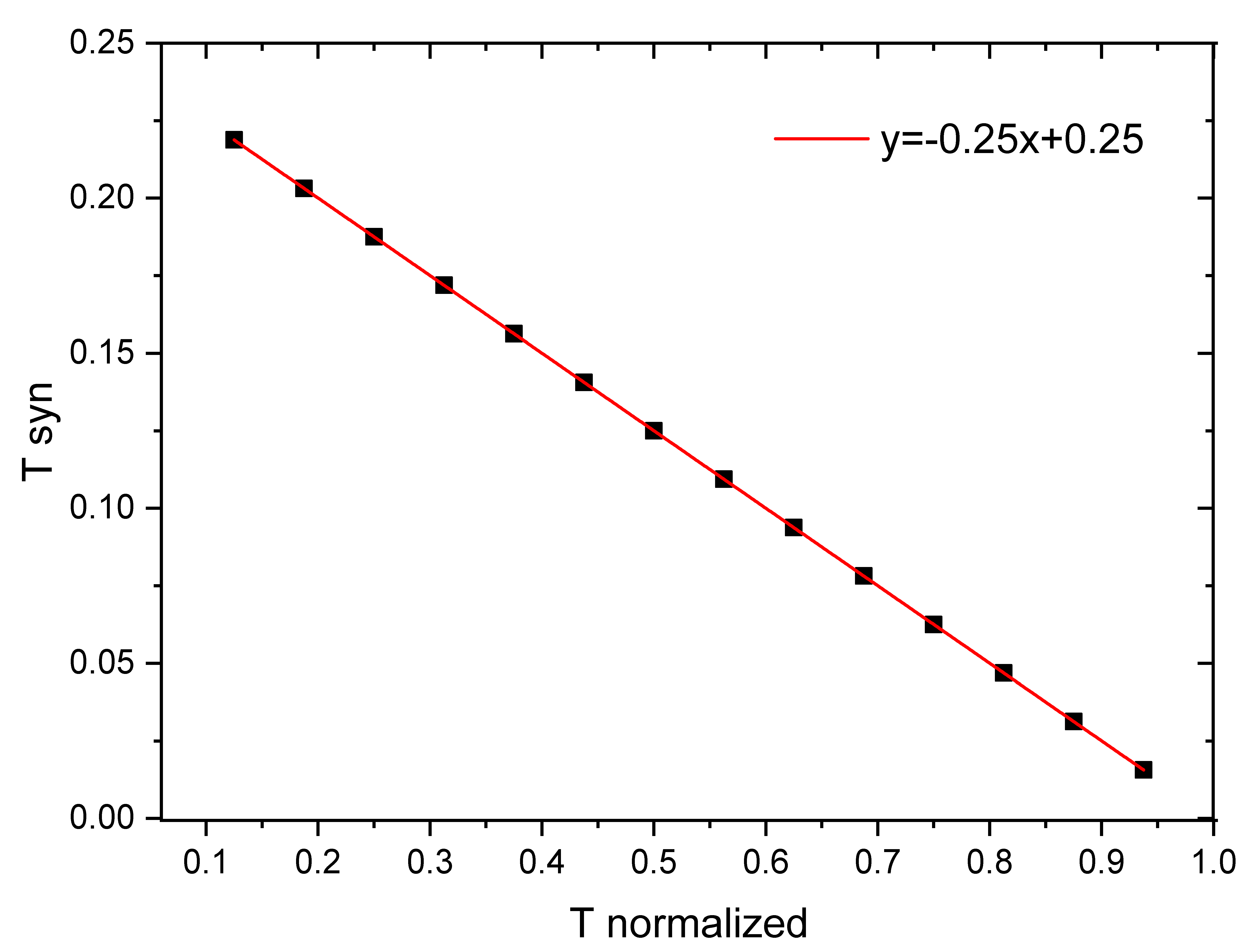
| Age T (Myr) | T Normalized | (-Values) |
|---|---|---|
| 20 | 0.125 | 0.219 |
| 30 | 0.188 | 0.203 |
| 40 | 0.250 | 0.188 |
| 50 | 0.313 | 0.172 |
| 60 | 0.375 | 0.156 |
| 70 | 0.438 | 0.141 |
| 80 | 0.500 | 0.125 |
| 90 | 0.563 | 0.109 |
| 100 | 0.625 | 0.094 |
| 110 | 0.688 | 0.078 |
| 120 | 0.750 | 0.063 |
| 130 | 0.813 | 0.047 |
| 140 | 0.875 | 0.031 |
| 150 | 0.938 | 0.016 |
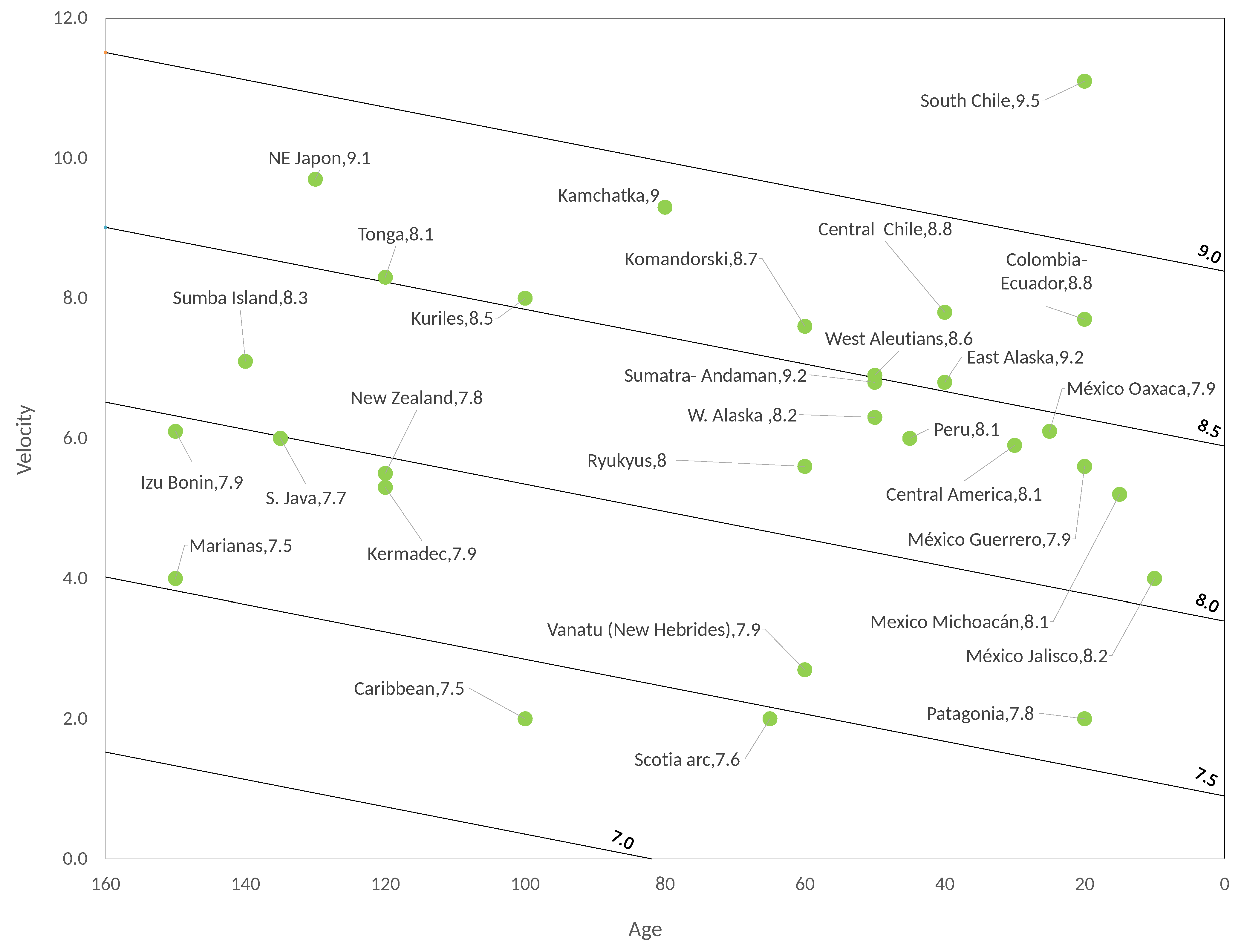
| Subduction Seismic Region | Subduction Rate V (cm/Year) | Magnitude of the Maximum Reported Earthquake | Age (Myr) | Calculated |
|---|---|---|---|---|
| East Alaska [23,24] | 6.8 | 9.2 | 40 | 8.5 |
| West Aleutians [23] | 6.9 | 8.6 | 50 | 8.5 |
| Sumatra-Andaman [25] | 6.8 | 9.2 | 50 | 8.5 |
| Central Chile [26,27] | 7.8 | 8.8 | 40 | 8.7 |
| South Chile [3,26,27] | 11.1 | 9.5 | 20 | 9.5 |
| Marianas [17] | 4 | 7.5 | 150 | 7.5 |
| Peru [28] | 6.0 | 8.1 | 45 | 8.3 |
| Tonga [17,26,29,30] | 8.3 | 8.1 | 120 | 8.5 |
| Colombia-Ecuador [3,31] | 7.7 | 8.8 | 20 | 8.8 |
| Central America [21,28,32] | 5.9 | 8.1 | 30 | 8.4 |
| NE Japan [3,33] | 9.7 | 9.1 | 130 | 8.8 |
| Kamchatka [3] | 9.3 | 9 | 80 | 8.9 |
| S. Java [34,35] | 6.0 | 7.7 | 135 | 8.0 |
| Izu Bonin [3,36] | 6.1 | 7.9 | 150 | 8.0 |
| Kermadec [37] | 5.3 | 7.9 | 120 | 7.9 |
| Kuriles [29] | 8 | 8.5 | 100 | 8.5 |
| New Zealand [3,38] | 5.5 | 7.8 | 120 | 8.0 |
| Vanatu (New Hebrides) [3,39] | 2.7 | 7.9 | 60 | 7.6 |
| Ryukyus [40,41] | 5.6 | 8 | 60 | 8.2 |
| Caribbean [3,42] | 2 | 7.5 | 100 | 7.3 |
| Scotia arc [3,43] | 2 | 7.6 | 65 | 7.5 |
| W. Alaska [23,26] | 6.3 | 8.2 | 50 | 8.4 |
| Komandorski [23,26] | 7.6 | 8.7 | 60 | 8.6 |
| Patagonia [17,43] | 2 | 7.8 | 20 | 7.6 |
| México- Jalisco [21,26,28] | 4 | 8.2 | 10 | 8.1 |
| Mexico-Michoacán [21,26,28] | 5.2 | 8.1 | 15 | 8.3 |
| México- Guerrero [21,26,28] | 5.6 | 7.9 | 20 | 8.4 |
| México- Oaxaca [21,26,28] | 6.1 | 7.9 | 25 | 8.4 |
| Sumba Island [34,44] | 7.1 | 8.3 | 140 | 8.2 |
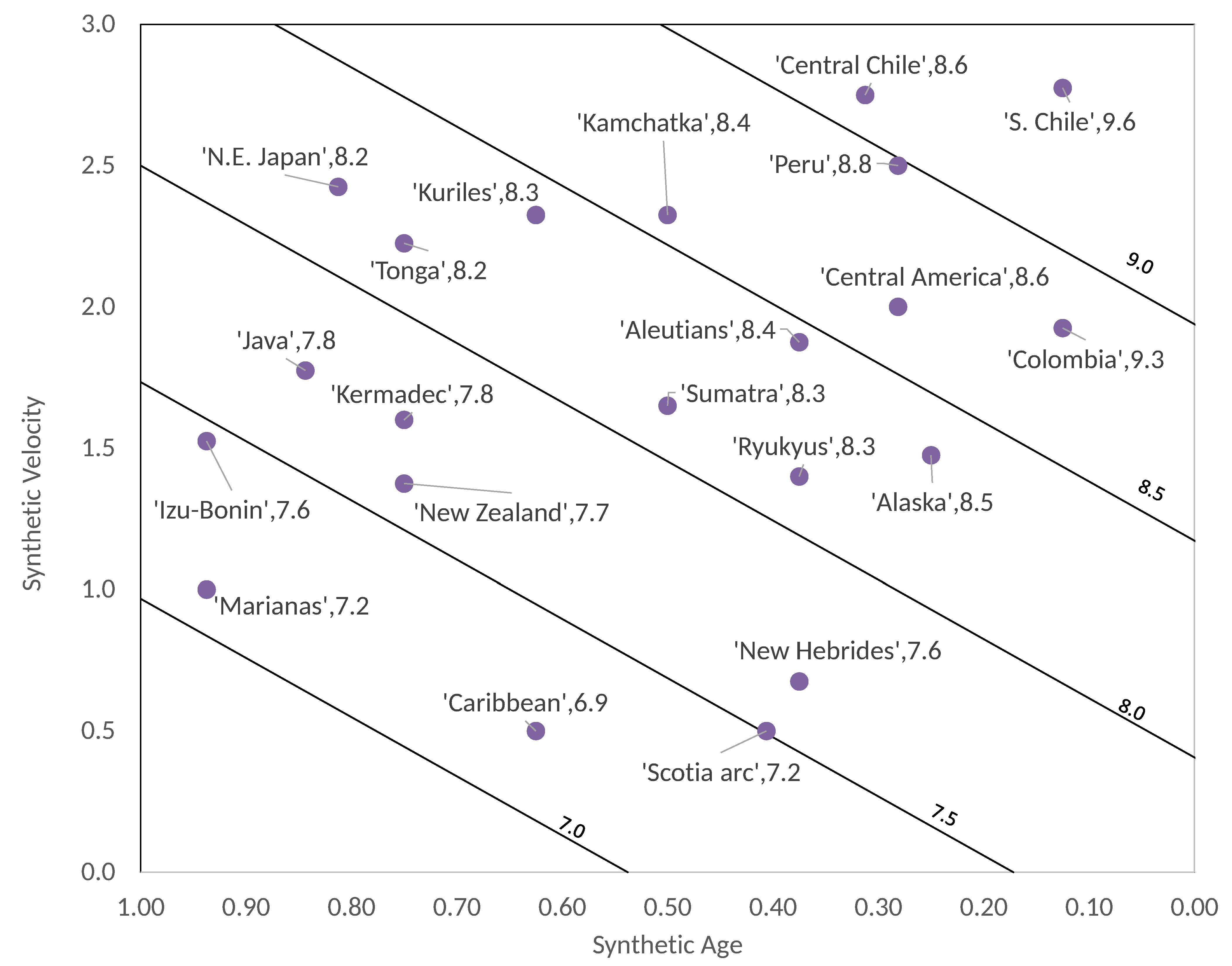
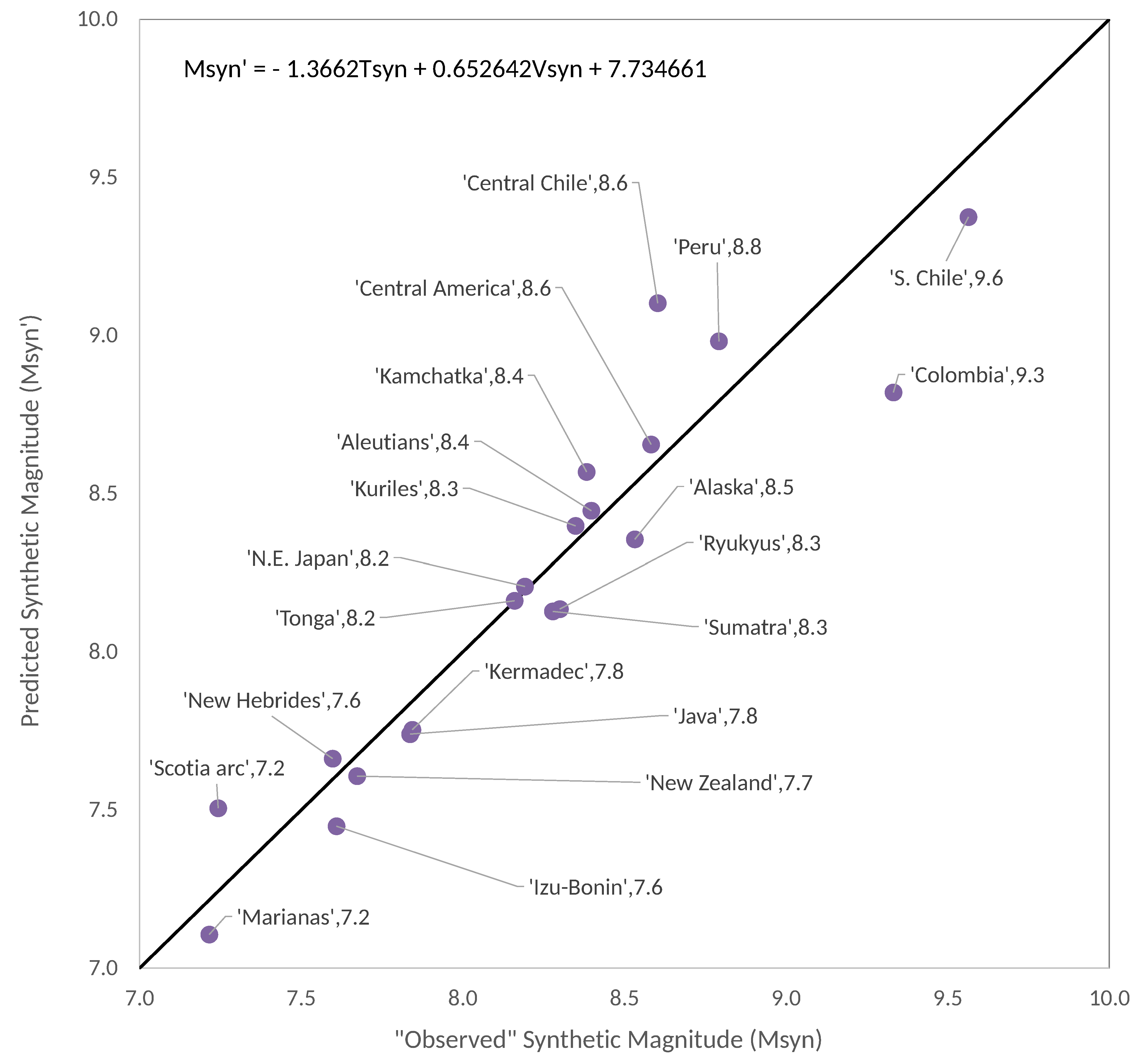
| Subduction Seismic Region | Tsyn (Gamma) | Normalized Age en | Vsyn | Maximum Size (m) of Synthetic Earthquake | Observed | Predicted Msyn′ |
|---|---|---|---|---|---|---|
| East Alaska | 0.188 | 0.25 | 1.700 | 13,084 | 8.6 | 8.7 |
| West Aleutians | 0.172 | 0.31 | 1.725 | 10,352 | 8.4 | 8.6 |
| Sumatra-Andaman | 0.172 | 0.31 | 1.700 | 10,283 | 8.4 | 8.6 |
| Central Chile | 0.188 | 0.25 | 1.950 | 15,020 | 8.8 | 8.9 |
| South Chile | 0.219 | 0.13 | 2.775 | 36,428 | 9.6 | 9.7 |
| Marianas | 0.016 | 0.94 | 1.000 | 2738 | 7.2 | 7.0 |
| Peru | 0.180 | 0.28 | 1.500 | 10,572 | 8.4 | 8.6 |
| Tonga | 0.063 | 0.75 | 2.075 | 7099 | 8.1 | 8.1 |
| Colombia-Ecuador | 0.219 | 0.13 | 1.925 | 28,450 | 9.3 | 9.1 |
| Central America | 0.203 | 0.19 | 1.475 | 14,301 | 8.7 | 8.7 |
| NE Japan | 0.047 | 0.81 | 2.425 | 7959 | 8.2 | 8.2 |
| Kamchatka | 0.125 | 0.50 | 2.325 | 9994 | 8.4 | 8.7 |
| S. Java | 0.039 | 0.84 | 1.500 | 4561 | 7.7 | 7.5 |
| Izu Bonin | 0.016 | 0.94 | 1.525 | 4216 | 7.6 | 7.3 |
| Kermadec | 0.063 | 0.75 | 1.325 | 4598 | 7.7 | 7.6 |
| Kuriles | 0.094 | 0.63 | 2.000 | 8405 | 8.2 | 8.2 |
| New Zealand | 0.063 | 0.75 | 1.375 | 4610 | 7.7 | 7.6 |
| Vanatu (New Hebrides) | 0.156 | 0.38 | 0.675 | 4187 | 7.6 | 7.8 |
| Ryukyus | 0.156 | 0.38 | 1.400 | 9043 | 8.3 | 8.3 |
| Caribbean | 0.094 | 0.63 | 0.500 | 1832 | 6.8 | 7.2 |
| Scotia arc | 0.148 | 0.41 | 0.500 | 2786 | 7.2 | 7.6 |
| W. Alaska | 0.172 | 0.31 | 1.575 | 10,054 | 8.4 | 8.5 |
| Komandorski | 0.156 | 0.38 | 1.900 | 10,124 | 8.4 | 8.6 |
| Patagonia | 0.219 | 0.13 | 0.500 | 6298 | 8.0 | 8.2 |
| Mexico-Jalisco | 0.234 | 0.06 | 1.000 | 29,780 | 9.4 | 8.6 |
| Mexico-Michoacán | 0.227 | 0.09 | 1.300 | 26,583 | 9.3 | 8.8 |
| Mexico-Guerrero | 0.219 | 0.13 | 1.400 | 21,842 | 9.1 | 8.8 |
| Mexico-Oaxaca | 0.211 | 0.16 | 1.525 | 18,605 | 8.9 | 8.8 |
| Sumba Island | 0.031 | 0.88 | 1.775 | 5175 | 7.8 | 7.6 |
© 2020 by the authors. Licensee MDPI, Basel, Switzerland. This article is an open access article distributed under the terms and conditions of the Creative Commons Attribution (CC BY) license (http://creativecommons.org/licenses/by/4.0/).
Share and Cite
Perez-Oregon, J.; Muñoz-Diosdado, A.; Rudolf-Navarro, A.H.; Angulo-Brown, F. A Simple Model to Relate the Elastic Ratio Gamma of a Critically Self-Organized Spring-Block Model with the Age of a Lithospheric Downgoing Plate in a Subduction Zone. Entropy 2020, 22, 868. https://doi.org/10.3390/e22080868
Perez-Oregon J, Muñoz-Diosdado A, Rudolf-Navarro AH, Angulo-Brown F. A Simple Model to Relate the Elastic Ratio Gamma of a Critically Self-Organized Spring-Block Model with the Age of a Lithospheric Downgoing Plate in a Subduction Zone. Entropy. 2020; 22(8):868. https://doi.org/10.3390/e22080868
Chicago/Turabian StylePerez-Oregon, Jennifer, Alejandro Muñoz-Diosdado, Adolfo Helmut Rudolf-Navarro, and Fernando Angulo-Brown. 2020. "A Simple Model to Relate the Elastic Ratio Gamma of a Critically Self-Organized Spring-Block Model with the Age of a Lithospheric Downgoing Plate in a Subduction Zone" Entropy 22, no. 8: 868. https://doi.org/10.3390/e22080868
APA StylePerez-Oregon, J., Muñoz-Diosdado, A., Rudolf-Navarro, A. H., & Angulo-Brown, F. (2020). A Simple Model to Relate the Elastic Ratio Gamma of a Critically Self-Organized Spring-Block Model with the Age of a Lithospheric Downgoing Plate in a Subduction Zone. Entropy, 22(8), 868. https://doi.org/10.3390/e22080868