Abstract
Based on the framework of our previous work [H.L. Lai et al., Phys. Rev. E, 94, 023106 (2016)], we continue to study the effects of Knudsen number on two-dimensional Rayleigh–Taylor (RT) instability in compressible fluid via the discrete Boltzmann method. It is found that the Knudsen number effects strongly inhibit the RT instability but always enormously strengthen both the global hydrodynamic non-equilibrium (HNE) and thermodynamic non-equilibrium (TNE) effects. Moreover, when Knudsen number increases, the Kelvin–Helmholtz instability induced by the development of the RT instability is difficult to sufficiently develop in the later stage. Different from the traditional computational fluid dynamics, the discrete Boltzmann method further presents a wealth of non-equilibrium information. Specifically, the two-dimensional TNE quantities demonstrate that, far from the disturbance interface, the value of TNE strength is basically zero; the TNE effects are mainly concentrated on both sides of the interface, which is closely related to the gradient of macroscopic quantities. The global TNE first decreases then increases with evolution. The relevant physical mechanisms are analyzed and discussed.
1. Introduction
Rayleigh–Taylor (RT) instability is widespread in nature and industry. It arises that, when a light fluid supports or pushes a heavy one (that is, when there are acceleration points from a heavy density fluid to a light one), a physical phenomenon in which disturbances at the interface increase with time [1]. RT instability plays a very important role in many fields: for example, in the inertial confinement fusion (ICF) [2,3,4], the supernova explosion [5], the Z-pinch plasma [6], the quantum magnetized plasma [7], the colloid admixture [8], and so on. There has been a handful of reported experiments [9,10,11,12,13] to describe RT instability, and great results have been achieved. However, due to the harsh experimental conditions, many researchers prefer to resort to numerical approaches to study RT instability, such as the unified decomposition method [14], the flux-corrected transport [15], the finite element method [16], the front tracking method [17], the monte carlo method [18], the polyphase moving particle semi-implicit method [19], smoothed particle hydrodynamics method [20], etc. In 1988, Grtar et al. proposed a two-way coupled Euler–Lagrange method to simulate the motion of non-viscous fluid interfaces with different densities, and it was applied to the study of RT instability [21]. In 2004, Miles et al. studied the effect of initial conditions on the two-dimensional (2D) RT instability and excessive turbulence of a planar detonation wave drive system, and obtained that the existence of short-wavelength components plays an important role in turbulent transitions, but its effect on large scale does not depend on its spectral properties [22]. In 2009, Banerjee et al. used the direct numerical simulation to study the RT instability of three-dimensional (3D) incompressible miscible fluids [23]. In 2012, Ye et al. considered non-spin incompressible inviscid fluids and analyzed the RT instability of the discontinuous distribution of the interface by analytical methods [24]. In 2015, Rozanov et al. studied the effect of initial conditions on RT instability, and it was obtained that the initial disturbance promoted the formation of a large number of 2D structures in the fluid [25]. In the same year, Sagert et al. used a modified direct simulation Monte Carlo method to study single-mode RT instability for a large range of Knudsen numbers [26]. In 2016, Yan et al. studied the nonlinear evolution of single-mode ablation RT instability in the 3D case, when the mode wavelength approaches the cutoff point of the linear spectrum, they found that the velocity of 3D saturated bubble is much faster than that of 2D bubble and classical 3D bubble [27]. In the same year, Zhou et al. used a numerical method to analyze the statistics of the kinetic energy and thermal energy dissipation rate of 2D RT turbulence [28]. Aslangil et al. used an implicit large eddy simulation technique to analyze the effect of initial conditions on the stability of miscible incompressible barotropic pressure driven RT under non-uniform acceleration conditions [29]. In 2018, Zhang et al. studied the instability of 2D and 3D multimode ablation RT. The simulation results showed that, under the condition of the same initial disturbance amplitude, the instability of nonlinear ablation RT was controlled by bubble competition. Compared with the classical scenario, a large amount of ablation could reduce the growth of nonlinear bubbles [30]. In 2019, based on compressible Navier–Stokes (NS) equations, Hu et al. studied the effect of viscosity on 2D single-mode RT instability during and after the re-acceleration stage [31]. In the same year, Kord et al. adopted a discrete-based adjoint method to control multimode RT instability by controlling the disturbance at the initial interface [32]. Liu et al. considered the single-mode classical RT instability of any Atwood number in the weakly nonlinear stage and studied the effect of mode coupling branches on harmonic amplitudes by means of modal coupling tracking technology [33]. Doludenko et al. analyzed the RT instability in the inviscous and viscous situations by performing direct numerical simulations of the Euler equation and the NS equations [34]. In 2020, Luo et al. used the finite difference method to simulate the late-time evolution of single-mode RT instability for isothermal stratification to study effects of compressibility and Atwood number [35]. These studies provide a lot of useful information for understanding the physical mechanism of RT instability [36,37].
In terms of mesoscopic numerical simulation, the lattice Boltzmann (LB) method, originally developed from a special discrete form of Boltzmann equation, has been widely used to solve corresponding hydrodynamic equations in various complex fluids, such as incompressible flows [38,39,40,41], porous media [42,43,44], magnetohydrodynamics [45,46], nonlinear wave [47,48], microchannel flow [49,50,51], nanofluid [52], and multiphase flows [53]. There were also many LB works to study the RT instability, and some useful results were obtained. In 1999, He et al. proposed an LB scheme and simulated the RT instability of the multiphase flow in the nearly incompressible limit [54]. In 2010, Scagliarini et al. used a thermal LB model to study RT instability of compressible stratified flows [55]. In 2012, Li et al. studied incompressible multiphase flows by LB model with additional interfacial force, and numerical simulations were carried out including the RT instability [56]. In 2015, Wang et al. proposed a multiphase LB flux solver for incompressible multiphase flows with low and large density ratios, which is validated by several benchmark problems, including RT instability [57]. In 2016, Liang et al. investiged the LB simulation of 3D RT instability and studied the effect of Reynolds number on the interfacial dynamic and spike and bubble amplitudes in detail [58]. In 2017, Wei et al. proposed an efficient coupled LB model for incompressible flow in application of turbulence RT instability [59]. The next year, Yang et al. studied the behavior of thermal and viscous entropy generation of global quantities with time evolution in RT turbulence mixing through the LB method [60]. In 2019, Liang et al. used an incompressible LB model to study multi-mode immiscible RT instability with high Reynolds numbers [61].
To our knowledge, the above studies mainly focus on the hydrodynamic non-equilibrium (HNE) effects of RT instability, and neglect the thermodynamic non-equilibrium (TNE) effects during the evolution of RT instability. To better describe the TNE effects on RT instability, we turn to the discrete Boltzmann method (DBM) [62,63,64] which is from coarse-grained modeling of the Boltzmann equation. The coarse-grained modeling is a process where the most important elements are kept and others may be neglected according to physical problem under study. The physical quantities that we will use to describe the system behavior must keep the same values after the simplification. From molecular dynamics or Liouville equation to Boltzmann’s equation, to the Burnett, the NS equations and Euler equations, coarse-grained modeling is a process of gradually neglecting detailed information which become relatively less important with increasing the spatio-temporal scale used to investigate the system. Over the past years, the DBM has been efficiently applied to many fields and brought some new insights into the corresponding systems. For example, in 2017, Lin et al. proposed a multi-component DBM for premixed, nonpremixed, or partially premixed non-equilibrium reactive flows, and the model is suitable for both subsonic and supersonic flows with or without chemical reaction and/or external force [65]. In 2018, Xu et al. presented a theoretical framework for constructing a DBM with spherical symmetry in spherical coordinates to kinetically model implosion- and explosion-related phenomena [66]. Lin et al. employed the DBM to study the HNE and TNE effects of the chemical reactant around the detonation wave [67]. Zhang et al. proposed the discrete ellipsoidal statistical Bhatnagar–Gross–Krook (BGK) model to simulate non-equilibrium compressible flows with a flexible Prandtl number [68]. In 2019, Gan et al. studied the effects of viscosity and heat conduction on the Kelvin–Helmholtz (KH) instability through the DBM. The authors found the viscosity effects stabilize the KH instability and enhance both the local and global TNE intensities [69]. Lin et al. employed the DBM to investigate the KH instability and found the relaxation time always strengthens the global non-equilibrium, entropy of mixing, and free enthalpy of mixing [70]. Besides by theory, results of DBM have been confirmed and supplemented by results of molecular dynamics [71,72], direct simulation Monte Carlo [73], and experiment [65].
In recent studies, compressible RT instability is studied by the DBM. In 2016, Lai et al. investigated the interaction between HNE and TNE effects using the DBM, and studied the effect of compressibility on 2D RT instability [74]. In the same year, Chen et al. used a multi-relaxation-time DBM to investigate the effects of viscosity, heat conductivity, and Prandtl number on the 2D RT instability from macroscopic and non-equilibrium viewpoints, and found that viscosity and heat conduction suppress RT instability mainly by suppressing the re-acceleration phase KH instability [75]. In 2017, Lin et al. extended the DBM to the compressible system containing two components with independent specific-heat ratios, and studied the dynamic process of the RT instability with two components [76]. In 2018, Chen et al. adopted a multi-relaxation-time DBM to numerically simulate a 2D Richtmyer–Meshkov (RM) instability and RT instability coexisting system [77]. Around the same time, Li et al. used the DBM to study the multi-mode RT instability with discontinuous interface in a compressible flow [78]. In 2019, Zhang et al. made a Lagrangian tracking supplement to the DBM, and studied the RT instability of the two-miscible-fluid system [79]. Despite the aforementioned efforts, there are still many problems needed to be studied. Based on previous work [74], in the following, we focus on the HNE and TNE behaviors, and aim to demonstrate the effects of the Knudsen number on the onset and growth of the 2D RT instability.
The content of this paper is organized as follows. In the next section, we briefly illustrate the DBM used in this work. The HNE and TNE behaviors about the 2D RT instability and the effects of Knudsen number are studied in Section 3. Finally, the research conclusions of this paper have been summarized and its further studies forecasted.
2. Discrete Boltzmann Model
The Boltzman equation of BGK collision with an external force [80] is:
where represents the distribution function of a single particle, the spatial coordinates, the velocity of particle, t the time, the relaxation time, the external force, and the local equilibrium distribution function. The expression of is as follows [81]:
where is a free parameter, D is the dimension of space, , T, and represent density, temperature, and fluid velocity, respectively. n is the number of extra degrees of freedom corresponding to molecular rotation and/or internal vibration.
In the Boltzmann equation with the BGK collision term, the particle velocity distribution function is replaced by the discrete velocity distribution function. It can be assumed that the system is very close to the equilibrium state, so f in the external term can be replaced by . Then, we can obtain the discrete Boltzmann equation with an external force term:
where and represent the discrete distribution function and discrete equilibrium distribution function corresponding to the i-th discrete velocity , with . The discrete local equilibrium distribution function should satisfy the following seven relationships:
where is Kronecker delta function, and , indicate either the x or y component. is the unit vector in the direction.
The above seven relationships can be written in a matrix form as follows (the boldface symbols denote N-dimensional column vectors):
where
where in two dimensions in the present model, , , , , , , , , , , , , , , , . , , , , , , , , , , , , , , , .
If the inverse of the matrix exists, then the discrete equilibrium distribution function is expressed as:
so the choice of discrete velocity model (DVM) has a high degree of flexibility which results in higher efficiency and better stability of this approach [63].
According to the conservations of mass, momentum, and energy, we have the following relationships:
By means of the Chapman–Enskog multiscale analysis, we can get the compressible NS equations from the DBM as follows:
where
and the pressure is
the total internal energy is
the dynamic viscosity coefficient is
the thermal conductivity viscosity coefficient is
In this way, we obtain the distribution function by solving the discrete Boltzmann Equation (3), then get the macro quantity through Equation (16), get the macro quantity by Equation (17), and get the macro quantity T by Equation (18).
Here, the following DVM (D2V16) is adopted:
where , , and , . c is the magnitude of the particle velocity in the first circle. The DVM of D2V16 is shown as Figure 1.
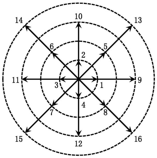
Figure 1.
Schematic diagram of D2V16 for DVM.
The DVM of D2V16 gets rid of the binding between spatial and time discretization, makes the particle velocity flexible, and it is convenient to introduce various computational methods to solve the discrete Boltzmann equation (3). The DBM is considered to be a special discrete form of the Boltzmann equation, and naturally inherits the properties of Boltzmann equation that can be used to describe TNE effects. Among the seven kinetic moment relations (4)–(10), only for the first three ones, can be replaced by . This is because, in or out of the equilibrium, the mass, momentum, and energy conservations are kept. However, the other four kinetic moment relations, if is replaced by , the two sides of these equations might not be equal, and some deviations will appear. From a physical point of view, these deviations are caused by the system deviating from the local equilibrium state. In this paper, we consider the TNE effects of the thermal fluctuation characteristics of micro-particles with macroscopic flow removed. The corresponding center moment are defined as:
where . In order to qualitatively analyze the evolution of TNE effects, we further define the total average TNE effects or intensity:
where represents the absolute average of the full field for each TNE effect which is defined as follows:
3. Numerical Simulations
In this section, we focus on the 2D compressible RT instability. The starting configuration is in a 2D domain . The entire system is in a gravitational field with constant gravitational acceleration, and the initial disturbance of the interface satisfies , k is the wave number and , is the wavelength. We create different layers of density by setting different temperatures. The temperatures of two half layers are initially set to constant, then the system satisfies by the hydrostatic equilibrium condition:
and therefore we have the initial hydrostatic unstable condition as:
where is the pressure at the top boundary at the beginning. and are the constant temperatures of the upper and bottom half parts, respectively. On this condition, we have the same static pressure at the disturbance interface:
where and are the densities of the upper and bottom grid aside the disturbance interface. Furthermore, the initial Atwood number is defined as follows:
In our simulations, the boundary conditions used in this work are as follows: the adiabatic and non-slip boundary conditions are used for the upper and lower boundaries; and symmetrical boundary conditions are used for the left and right sides.
Here, as in the previous work [74], we choose the units of length and time as and , respectively, then the unit of velocity is , so we have two dimensionless parameters as follows:
and
where describes the compressibility of the flow, describes the ratio of the relaxation time, and a macroscopic time. It can be deduced obviously that can represent the Knudsen number. In addition, works as a parameter to roughly describe how far the system deviates from its thermodynamic equilibrium in the initial state. In addition, not only that, also describes the relative strength of dissipation work rate over mechanical work rate. To study the Knudsen number , we should make sure the compressibility number is constant.
In the present work, the calculation area we adopted is a uniform grid of , the space step , the time step , then . The initial pressure at the top , the upper part temperature and the lower part temperature are , , then . Other parameters are , , , , . We calculate the value of by the initial temperature in the upper part as , then we can calculate the compressibility . We can change the relaxation time to change the Kundsen number .
In order to observe the evolution of the 2D RT instability with time more intuitively, the density evolution is shown in Figure 2. We choose three relaxation times: , , , corresponding to three Knudsen numbers: , and , respectively. These simulation results show that, for all values, due to the effects of the gravity, the disturbance interface is rolled up at the tip or peak, and then two pairs of opposite vortices are formed. The perturbation interfaces all evolved into the shapes of “bubble” and “spike”. Here, the structure of rising lighter fluid is referred to as bubble, and the structure of falling heavier fluid is referred to as spike. We also find that the smaller the , the faster the roll-up phenomenon appears. Moreover, the smaller with value, the stronger influence of KH instability on the later stage, the vortex will further develop, become longer, and form two pairs of long rolls, finer structures appear. When the spike approaches the lower wall, the lower part of the bubble is deflected downward while the upper part keeps moving up, maintaining the “mushroom” shape. As the value increases, the size of the vortex decreases significantly, these rolls squeeze the light fluid inward, and then contact the heavy fluid, the spike tail is flipped up to form a mushroom shape, at which time the nonlinear effect is very strong. At the same time, we observe that, in the initial stage, the thermal diffusion quickly smoothes the discontinuous, and the larger , the stronger thermal diffusion.
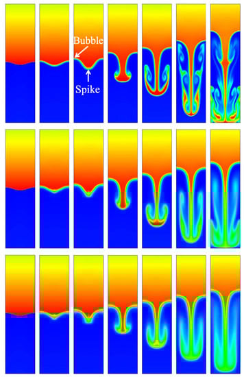
Figure 2.
Evolution of the density contour at time instants (from left to right) , , , , , , and , respectively. The three rows, from top to bottom, correspond to the cases with Knudsen numbers , , and , respectively. When increases, the inhibition effect becomes more obvious.
In general, the thickness of the mixed layer is an important parameter to measure the evolution of RT instability. We track the positions of bubble and spike as an indicator of the mixed layer, and define half the distance between the bubble and the spike as the amplitude. In order to study the effect of on RT instability, we use the local TNE quantity to track the position of spike and bubble [74]. In order to study the effect of Knudsen number on the RT instability of compressible fluid, we can adjust the dimensionless Knudsen number through by Equation (34). We choose six different values , , , , , , corresponding to six different as , , , , , . The results are shown in Figure 3 and Figure 4. Here, . Figure 3 displays the time evolutions of the spike with the dimensionless Knudsen number . From the evolution of the spike, we can find that the Knudsen number tends to inhibit the RT instability. Figure 4 displays the time evolutions of the bubble with the dimensionless Knudsen number . It is interesting to observe that, when , with the increase of , the larger , the faster it goes down. Meanwhile, from to and to , the bubble grows exponentially, and from to , the growth rate is faster than from to . This phenomenon can be understood as first the system in the adjustment phase, then the stored compressive energy of the system is released into kinetic energy. As the Kundsen number gets larger, the collision time of particles in the system gets longer, and the conversion between energies also gets longer. Figure 5 shows the growth of the amplitude with different values of the Knudsen number. The effect of in the prophase is not significant, while later the effect gradually emerged. It can be found that the effects of Knudsen number stabilize the RT instability as a whole.
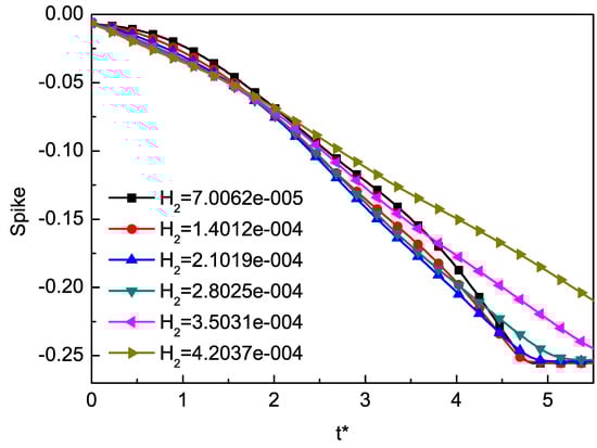
Figure 3.
The time evolutions of the spike at different values of Knudsen number . The Knudsen number tends to inhibit the RT instability.
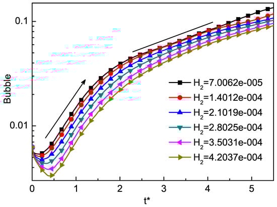
Figure 4.
The growth of the bubble by the DBM. The good linear fit is consistent with the growth of the bubble at the beginning.
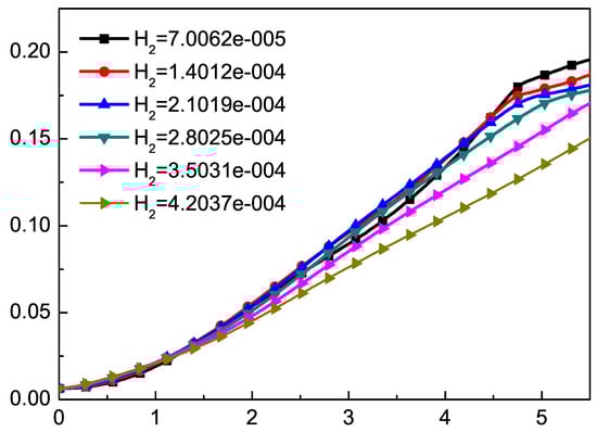
Figure 5.
The growth of the amplitude with different values of the Knudsen number. The effect of in the prophase is not significant, while later the effect gradually emerged.
The time evolution of the total average TNE strength of the RT instability with different values of Knudsen number are shown in Figure 6. It is interesting to find that the total average TNE strength first decreases in the first stage and then increases in the later stage for each . Furthermore, the higher the Knudsen number, the stronger the total average TNE effects. Note that, as is increased, the linear stage of growth is prolonged in time, then the total average TNE strength tends to a constant.
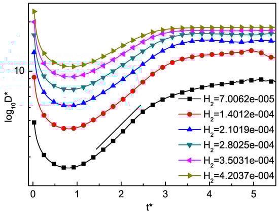
Figure 6.
The time evolution of the total average TNE strength with different values of Knudsen number . The total average TNE strength first decreases in the first stage and then increases in the later stage for each . The higher the Knudsen number, the stronger the total average TNE effects.
In Figure 7, we illustrate the profiles of each TNE quantity. We find that the description of non-equilibrium characteristics is not identical. Each TNE component is embodied in a certain degree of freedom, and different degrees of freedom have different physical meanings. is the degree to which the internal energy of x degrees of freedom deviates from the equilibrium state, represents the non-equilibrium characterization associated with the shear effect, represents the flux of the internal energy in the x direction in the y degrees of freedom, represents the flux of internal energy in the y-direction at y degrees of freedom, represents the internal energy flux in the x direction, represents unorganized energy flow in the y direction, and represents the flux of internal energy flux. Far from the interface, the value of non-equilibrium strength is basically zero, and the non-equilibrium effect is mainly concentrated on both sides of the interface, which is closely related to the gradient of macroscopic quantities. Near the interface, the TNE effect is obvious and the intensity is large, indicating that the system at the interface deviates far from the thermodynamic equilibrium state. DBM provides an effective tool for the study of TNE non-equilibrium phenomena beyond the description of traditional hydrodynamic models, which just provides only the viscosity and the heat conduction effect.
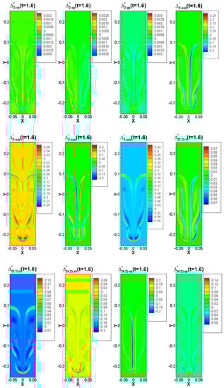
Figure 7.
Contours of various components of TNE effects at under the condition of . The TNE effects are mainly concentrated on the two sides of the interface, far away from the interface, and the TNE effect is basically zero. Some of the TNE effects are relatively smaller, some are larger, and some showed the opposite effect.
4. Conclusions
In this paper, based on our previous work [74], we continue to use the discrete Boltzmann method (DBM) to study the two-dimensional (2D) Rayleigh–Taylor (RT) instability in the compressible fluids. In the framework of our model, there are two dimensionless parameters, one represents the compressibility , and the other represents the Knudsen number . We focus on the latter. The hydrodynamic non-equilibrium (HNE) effects and the thermodynamic non-equilibrium (TNE) effects of the compressible RT instability are investigated by changing the non-dimensional parameter Knudsen number when the compressibility doesn’t change. 2D HNE and TNE effects are demonstrated in detail. We also investigate the “spike” and “bubble” of the 2D RT instability traced by the local non-equilibrium quantity . The effects of the Knudsen number on the developments of RT instability are carefully analyzed for six cases with the same initial perturbations. From the simulation results, we find that the Knudsen number plays an important role in the RT instability. The mixing-zone grows inversely with increasing the Knudsen number . At the same time, the larger , the more obvious the Kelvin–Helmholtz instability for the later development, and the faster the shape of the mushroom appears. Furthermore, different TNE quantities display a wealth of non-equilibrium information. Far from the disturbance interface, the value of non-equilibrium strength is basically zero, and the non-equilibrium effect is mainly concentrated on both sides of the interface, which is closely related to the gradient of macroscopic quantities. Near the interface, the various TNE effects are more obvious and the corresponding intensity are relatively large, indicating that the interface of the system deviates far from the thermodynamic equilibrium state. The observations on the HNE and TNE effects influenced by the effects of Kundsen number are helpful for a better understanding the process of RT instability on compressible fluids.
Author Contributions
Investigation, L.C.; Methodology, H.L.; Validation, D.L.; Visualization, Y.G.; Writing–original draft, H.Y.; Writing–review and editing, C.L. and A.X. All authors have read and approved the final manuscript.
Funding
This work was supported by the National Natural Science Foundation of China (under Grant Nos. 11301082, 11772064, 11875001, and 51806116), the Natural Science Foundation of Fujian Provinces (under Grant Nos. JT180075, 2018J01654) and CAEP Foundation under Grant No. CX2019033, and the opening project of State Key Laboratory of Explosion Science and Technology (Beijing Institute of Technology) under Grant No. KFJJ19-01M.
Conflicts of Interest
The authors declare no conflict of interest.
References
- Kull, H.J. Theory of the Rayleigh–Taylor instability. Phys. Rep. 1991, 206, 197–325. [Google Scholar] [CrossRef]
- Betti, R.; Goncharov, V.N.; McCrory, R.L.; Verdon, C.P. Growth rates of the ablative Rayleigh–Taylor instability in inertial confinement fusion. Phys. Plasmas 1998, 5, 1446–1454. [Google Scholar] [CrossRef]
- Lindl, J.D.; McCrory, R.L.; Campbell, E.M. Rogress toward ignition and burn propagation in inertial confinement fusion. Phys. Today 1992, 45, 32–40. [Google Scholar] [CrossRef]
- Wang, L.; Ye, W.; He, X.; Wu, J.; Fan, Z.; Xue, C.; Jia, G. Theoretical and simulation research of hydrodynamic instabilities in inertial-confinement fusion implosions. Sci. China Phys. Mech. 2017, 60, 055201. [Google Scholar] [CrossRef]
- Cabot, W.H.; Cook, A.W. Reynolds number effects on Rayleigh–Taylor instability with possible implications for type Ia supernovae. Nat. Phys. 2006, 2, 562–568. [Google Scholar] [CrossRef]
- Huang, L.; Jian, G.D.; Qiu, X.M.; Peng, X.D.; Wang, S.Q. Effects of compressibility on the finite Larmor radius stabilized Rayleigh–Taylor instability in Z-pinch implosions. Acta Phys. Sin. 2008, 15, 022103. [Google Scholar] [CrossRef]
- Wang, L.F.; Yang, B.L.; Ye, W.H.; He, X.T. Stabilization of the Rayleigh–Taylor instability in quantum magnetized plasmas. Phys. Plasmas 2012, 19, 072704. [Google Scholar]
- Milinković, K.; Padding, J.T.; Dijkstra, M. Hydrodynamic Rayleigh–Taylor-like instabilities in sedimenting colloidal mixtures. Soft Matter 2011, 7, 11177–11186. [Google Scholar]
- Park, H.S.; Lorenz, K.T.; Cavallo, R.M.; Pollaine, S.M.; Prisbrey, S.T.; Rudd, R.E.; Becker, R.C.; Bernier, J.V.; Remington, B.A. Viscous Rayleigh–Taylor instability experiments at high pressure and strain rate. Phys. Rev. Lett. 2010, 104, 135504. [Google Scholar] [CrossRef]
- White, J.; Oakley, J.; Anderson, M.; Bonazza, R. Experimental measurements of the nonlinear Rayleigh–Taylor instability using a magnetorheological fluid. Phys. Rev. E 2010, 81, 026303. [Google Scholar] [CrossRef]
- Wykes, M.S.D.; Dalziel, S.B. Efficient mixing in stratified flows: Experimental study of a Rayleigh–Taylor unstable interface within an otherwise stable stratification. J. Fluid Mech. 2014, 756, 1027–1057. [Google Scholar] [CrossRef]
- Rigon, G.; Casner, A.; Albertazzi, B.; Michel, T.; Mabey, P.; Falize, E.; Ballet, J.; Som, L.V.B.; Pikuz, S.; Sakawa, Y.; et al. Rayleigh–Taylor instability experiments on the LULI2000 laser in scaled conditions for young supernova remnants. Phys. Rev. E 2019, 100, 021201. [Google Scholar] [CrossRef] [PubMed]
- Polavarapu, R.; Roach, P.; Banerjee, A. Rayleigh–Taylor-instability experiments with elastic-plastic materials. Phys. Rev. E 2019, 99, 053104. [Google Scholar] [CrossRef] [PubMed]
- Sun, Y.B.; Tao, J.J.; He, X.T. Unified decomposition method to study Rayleigh–Taylor instability in liquids and solids. Phys. Rev. E 2018, 97, 063109. [Google Scholar] [CrossRef] [PubMed]
- Ye, W.H.; Zhang, W.Y.; Chen, G.N.; Jin, C.Q.; Zhang, J. Numerical simulations of the FCT method on Rayleigh–Taylor and Richtmyer-Meshkov instabilities. Chin. J. Comput. Phys. 1998, 15, 277. [Google Scholar]
- Dervieux, A.; Thomasset, F. A finite element method for the simulation of a Rayleigh–Taylor instability. In Approximation Methods for Navier–Stokes Problems; Rautmann, R., Ed.; Lecture Notes in Mathematics; Springer: Berlin/Heidelberg, Germany, 1980; Volume 771, pp. 145–158. [Google Scholar]
- Terashima, H.; Tryggvason, G. A front-tracking/ghost-fluid method for fluid interfaces in compressible flows. J. Comput. Phys. 2009, 228, 4012–4037. [Google Scholar] [CrossRef]
- Gallis, M.A.; Koehler, T.P.; Torczynski, J.R.; Plimpton, S.J. Direct simulation Monte Carlo investigation of the Rayleigh–Taylor instability. Phys. Rev. Fluids 2016, 1, 043403. [Google Scholar] [CrossRef]
- Guo, K.L.; Chen, R.H.; Li, Y.L.; Tian, W.X.; Su, G.H.; Qiu, S.Z. Numerical simulation of Rayleigh–Taylor Instability with periodic boundary condition using MPS method. Prog. Nucl. Energ. 2018, 109, 130–144. [Google Scholar] [CrossRef]
- Shadloo, M.S.; Zainali, A.; Yildiz, M. Simulation of single mode Rayleigh–Taylor instability by SPH method. Comput. Mech. 2013, 51, 699. [Google Scholar] [CrossRef]
- Tryggvason, G. Numerical Simulations of the Rayleigh–Taylor Instability. J. Comput. Phys. 1998, 75, 253–282. [Google Scholar] [CrossRef]
- Miles, A.R.; Edwards, M.J.; Greenough, J.A. Effect of initial conditions on two-dimensional Rayleigh–Taylor instability and transition to turbulence in planar blast-wave-driven systems. Phys. Plasmas 2004, 11, 5278–5296. [Google Scholar] [CrossRef]
- Banerjee, A.; Andrews, M.J. 3D Simulations to investigate initial condition effects on the growth of Rayleigh–Taylor mixing. Int. J. Heat. Mass Tran. 2009, 52, 3906–3917. [Google Scholar] [CrossRef]
- Liu, W.H.; Wang, L.F.; Ye, W.H.; He, X.T. Nonlinear saturation amplitudes in classical Rayleigh–Taylor instability at arbitrary Atwood numbers. Phys. Plasmas 2012, 19, 042705. [Google Scholar]
- Rozanov, V.B.; Kuchugov, P.A.; Zmitrenko, N.V.; Yanilkin, Y.V. Effect of initial conditions on the development of Rayleigh–Taylor instability. J. Russ. Laser Res. 2015, 36, 139–150. [Google Scholar] [CrossRef]
- Sagert, I.; Howell, J.; Staber, A.; Strother, T.; Colbry, D.; Bauer, W. Knudsen-number dependence of two-dimensional single-mode Rayleigh–Taylor fluid instabilities. Phys. Rev. E. 2015, 92, 013009. [Google Scholar] [CrossRef]
- Yan, R.; Betti, R.; Sanz, J.; Aluie, H.; Liu, B.; Frank, A. Three-dimensional single-mode nonlinear ablative Rayleigh–Taylor instability. Phys. Plasmas 2016, 23, 022701. [Google Scholar] [CrossRef]
- Zhou, Q.; Jiang, L.F. Kinetic and thermal energy dissipation rates in two-dimensional Rayleigh–Taylor turbulence. Phys. Fluids 2016, 28, 045109. [Google Scholar] [CrossRef]
- Aslangil, D.; Banerjee, A.; Lawrie, A.G.W. Numerical investigation of initial condition effects on Rayleigh–Taylor instability with acceleration reversals. Phys. Rev. E 2016, 94, 053114. [Google Scholar] [CrossRef]
- Zhang, H.; Betti, R.; Yan, R.; Zhao, D.; Shvarts, D.; Aluie, H. Self-similar multimode bubble-front evolution of the ablative Rayleigh–Taylor instability in two and three dimensions. Phys. Rev. Lett. 2018, 121, 185002. [Google Scholar] [CrossRef]
- Hu, Z.X.; Zhang, Y.S.; Tian, B.; He, Z.; Li, L. Effect of viscosity on two-dimensional single-mode Rayleigh–Taylor instability during and after the reacceleration stage. Phys. Fluids 2019, 31, 104108. [Google Scholar]
- Kord, A.; Capecelatro, J. Optimal perturbations for controlling the growth of a Rayleigh–Taylor instability. J. Fluid Mech. 2019, 876, 150–185. [Google Scholar] [CrossRef]
- Liu, W.H.; Chen, Y.L.; Huang, Y.; Mei, Y.; Ye, W.H. Mode-coupling branches in single-mode classical Rayleigh–Taylor instability for arbitrary atwood numbers. Results Phys. 2019, 12, 1142–1148. [Google Scholar] [CrossRef]
- Doludenko, A.; Fortova, S.; Shepelev, V.; Son, E. Numerical simulation of the Rayleigh–Taylor instability of inviscid and viscous fluid. Phys. Scripta 2019, 94, 094003. [Google Scholar] [CrossRef]
- Luo, T.F.; Wang, J.C.; Xie, C.Y.; Wan, M.P.; Chen, S.Y. Effects of compressibility and Atwood number on the single-mode Rayleigh–Taylor instability. Phys. Fluids 2020, 31, 012110. [Google Scholar]
- Zhou, Y. Rayleigh–Taylor and Richtmyer-Meshkov instability induced flow, turbulence, and mixing. I. Phys. Rep. 2017, 720, 1–136. [Google Scholar]
- Zhou, Y. Rayleigh–Taylor and Richtmyer-Meshkov instability induced flow, turbulence, and mixing. II. Phys. Rep. 2017, 723, 1–160. [Google Scholar] [CrossRef]
- Peng, Y.; Shu, C.; Chew, Y.T. Simplified thermal lattice Boltzmann model for incompressible thermal flows. Phys. Rev. E 2003, 68, 026701. [Google Scholar] [CrossRef] [PubMed]
- Wei, Y.K.; Wang, Z.D.; Dou, H.S.; Qian, Y.H.; Yan, W.W. Simulations of natural convection heat transfer in an enclosure at different Rayleigh number using lattice Boltzmann method. Comput. Fluids 2016, 124, 30–38. [Google Scholar] [CrossRef]
- Wei, Y.K.; Yang, H.; Lin, Z.; Wang, Z.D.; Qian, Y.H. A novel two-dimensional coupled lattice Boltzmann model for thermal incompressible flows. Appl. Math. Comput. 2018, 339, 556–567. [Google Scholar] [CrossRef]
- Wang, Z.D.; Wei, Y.K.; Qian, Y.H. A bounce back-immersed boundary-lattice Boltzmann model for curved boundary. Appl. Math. Model. 2020, 81, 428–440. [Google Scholar] [CrossRef]
- Guo, Z.L.; Zhao, T.S. Lattice Boltzmann model for incompressible flows through porous media. Phys. Rev. E 2002, 66, 036304. [Google Scholar] [CrossRef] [PubMed]
- Liu, H.H.; Kang, Q.J.; Leonardi, C.R.; Schmieschek, S.; Narváez, A.; Jones, B.D.; Harting, J. Multiphase lattice Boltzmann simulations for porous media applications. Comput. Geosci. 2016, 20, 777–805. [Google Scholar] [CrossRef]
- He, Y.L.; Liu, Q.; Li, Q.; Tao, W.Q. Lattice Boltzmann methods for single-phase and solid-liquid phase-change heat transfer in porous media: A review. Int. J. Heat Mass Tran. 2016, 129, 160–197. [Google Scholar] [CrossRef]
- Chen, S.Y.; Chen, H.D.; Martnez, D.; Matthaeus, W. Lattice Boltzmann model for simulation of magnetohydrodynamics. Phys. Rev. Lett. 1991, 67, 3776–3779. [Google Scholar] [CrossRef] [PubMed]
- Dellar, P.J. Lattice Boltzmann magnetohydrodynamics with current-dependent resistivity. J. Comput. Phys. 2013, 237, 115–131. [Google Scholar] [CrossRef]
- Li, D.M.; Lai, H.L.; Shi, B.C. Mesoscopic simulation of the (2+1)-dimensional wave equation with nonlinear damping and source terms using the lattice Boltzmann BGK model. Entropy 2019, 21, 390. [Google Scholar] [CrossRef]
- Li, D.M.; Lai, H.L.; Lin, C.D. Mesoscopic simulation of the two-component system of coupled sine-Gordon equations with lattice Boltzmann method. Entropy 2019, 21, 542. [Google Scholar] [CrossRef]
- Lim, C.Y.; Shu, C.; Niu, X.D.; Chew, Y.T. Application of lattice Boltzmann method to simulate microchannel flows. Phys. Fluids 2002, 14, 2299–2308. [Google Scholar] [CrossRef]
- Tang, G.H.; Tao, W.Q.; He, Y.L. Lattice Boltzmann method for simulating gas flow in microchannels. Int. J. Mod. Phys. C 2004, 15, 335–347. [Google Scholar] [CrossRef]
- Li, Q.; He, Y.L.; Tang, G.H.; Tao, W.Q. Lattice Boltzmann modeling of microchannel flows in the transition flow regime. Microfluid. nanofluid. 2011, 10, 607–618. [Google Scholar] [CrossRef]
- Sheikholeslami, M.; Ganji, D.D. Entropy generation of nanofluid in the presence of magnetic field using Lattice Boltzmann Method. Phys. A 2015, 417, 273–286. [Google Scholar] [CrossRef]
- Li, Q.; Luo, K.H.; Kang, Q.J.; He, Y.L.; Chen, Q.; Liu, Q. Lattice Boltzmann methods for multiphase flow and phase-change heat transfer. Prog. Energ. Combust. 2016, 52, 62–105. [Google Scholar] [CrossRef]
- He, X.Y.; Chen, S.Y.; Zhang, R.Y. A lattice Boltzmann scheme for incompressible multiphase flow and its application in simulation of Rayleigh–Taylor instability. J. Comput. Phys. 1999, 152, 642–663. [Google Scholar] [CrossRef]
- Scagliarini, A.; Biferale, L.; Sbragaglia, M.; Sugiyama, K.; Toschi, F. Lattice Boltzmann methods for thermal flows: Continuum limit and applications to compressible Rayleigh–Taylor systems. Phys. Fluids 2010, 22, 055101. [Google Scholar] [CrossRef]
- Li, Q.; Luo, K.H.; Gao, Y.J.; He, Y.L. Additional interfacial force in lattice Boltzmann models for incompressible multiphase flows. Phys. Rev. E 2012, 85, 026704. [Google Scholar] [CrossRef]
- Wang, Y.; Shu, C.; Huang, H.B.; Teo, C.J. Multiphase lattice Boltzmann flux solver for incompressible multiphase flows with large density ratio. J. Comput. Phys. 2015, 280, 404–423. [Google Scholar] [CrossRef]
- Liang, H.; Li, Q.X.; Shi, B.C.; Chai, Z.H. Lattice boltzmann simulation of three-dimensional Rayleigh–Taylor instability. Phys. Rev. E 2016, 93, 033113. [Google Scholar] [CrossRef]
- Wei, Y.K.; Dou, H.S.; Qian, Y.H.; Wang, Z.D. A novel two-dimensional coupled lattice Boltzmann model for incompressible flow in application of turbulence Rayleigh–Taylor instability. J. Comput. Phys. 2017, 156, 97–102. [Google Scholar] [CrossRef]
- Yang, X.Y.; He, H.J.; Xu, J.; Wei, Y.K.; Zhang, H. Entropy generation rates in two-dimensional Rayleigh–Taylor turbulence mixing. Entropy 2018, 20, 738. [Google Scholar] [CrossRef]
- Liang, H.; Hu, X.L.; Huang, X.F.; Xu, J.R. Direct numerical simulations of multi-mode immiscible Rayleigh–Taylor instability with high Reynolds numbers. Phys. Fluids 2019, 31, 112104. [Google Scholar]
- Xu, A.G.; Zhang, G.C.; Gan, Y.B.; Chen, F.; Yu, X.J. Lattice Boltzmann modeling and simulation of compressible flows. Front. Phys. 2012, 7, 582–600. [Google Scholar] [CrossRef]
- Gan, Y.B.; Xu, A.G.; Zhang, G.C.; Yang, Y. Lattice BGK kinetic model for high-speed compressible flows: Hydrodynamic and non-equilibrium behaviors. Europhys. Lett. 2013, 103, 24003. [Google Scholar] [CrossRef]
- Xu, A.G.; Zhang, G.C.; Zhang, Y.D. Discrete Boltzmann Modeling of Compressible Flows. In Kinetic Theory; Kyzas, G.Z., Mitropoulos, A.C., Eds.; IntechOpen: London, UK, 2018; Chapter 2. [Google Scholar]
- Lin, C.D.; Luo, K.H.; Fei, L.L.; Succi, S. A multi-component discrete Boltzmann model for non-equilibrium reactive flows. Sci. Rep. 2017, 7, 14580. [Google Scholar] [CrossRef] [PubMed]
- Xu, A.G.; Zhang, G.C.; Zhang, Y.D.; Wang, P.; Ying, Y.J. Discrete Boltzmann model for implosion- and explosionrelated compressible flow with spherical symmetry. Front. Phys. 2018, 13, 135102. [Google Scholar] [CrossRef]
- Lin, C.D.; Luo, K.H. Mesoscopic simulation of non-equilibrium detonation with discrete Boltzmann method. Combust. Flame 2018, 198, 356–362. [Google Scholar] [CrossRef]
- Zhang, Y.D.; Xu, A.G.; Zhang, G.C.; Chen, Z.H.; Wang, P. Discrete ellipsoidal statistical BGK model and Burnett equations. Front. Phys. 2018, 13, 135101. [Google Scholar] [CrossRef]
- Gan, Y.B.; Xu, A.G.; Zhang, G.C.; Lin, C.D.; Lai, H.L.; Liu, Z.P. Nonequilibrium and morphological characterizations of Kelvin–Helmholtz instability in compressible flows. Front. Phys. 2019, 14, 43602. [Google Scholar] [CrossRef]
- Lin, C.D.; Luo, K.H.; Gan, Y.B.; Liu, Z.P. Kinetic simulation of non-equilibrium Kelvin–Helmholtz instability. Commun. Theor. Phys. 2019, 71, 132–142. [Google Scholar] [CrossRef]
- Liu, H.; Kang, W.; Zhang, Q.; Zhang, Y.; Duan, H.L.; He, X.T. Molecular dynamics simulations of microscopic structure of ultra strong shock waves in dense helium. Front. Phys. 2016, 11, 115206. [Google Scholar] [CrossRef]
- Liu, H.; Zhang, Y.; Kang, W.; Zhang, P.; Duan, H.L.; He, X.T. Molecular dynamics simulation of strong shock waves propagating in dense deuterium, taking into consideration effects of excited electrons. Phys. Rev. E 2016, 95, 023201. [Google Scholar] [CrossRef]
- Zhang, Y.D.; Xu, A.G.; Zhang, G.C.; Chen, Z.H.; Wang, P. Discrete Boltzmann method for non-equilibrium flows: Based on Shakhov model. Comput. Phys. Commun. 2019, 238, 50–65. [Google Scholar] [CrossRef]
- Lai, H.L.; Xu, A.G.; Zhang, G.C.; Gan, Y.B.; Ying, Y.J.; Succi, S. Nonequilibrium thermohydrodynamic effects on the Rayleigh–Taylor instability in compressible flows. Phys. Rev. E 2016, 94, 023106. [Google Scholar] [CrossRef] [PubMed]
- Chen, F.; Xu, A.G.; Zhang, G.C. Viscosity, heat conductivity, and Prandtl number effects in the Rayleigh–Taylor Instability. Front. Phys. 2016, 11, 114703. [Google Scholar] [CrossRef]
- Lin, C.D.; Xu, A.G.; Zhang, G.C.; Luo, K.H.; Li, Y.J. Discrete Boltzmann modeling of Rayleigh–Taylor instability in two-component compressible flows. Phys. Rev. E 2017, 96, 053305. [Google Scholar] [CrossRef] [PubMed]
- Chen, F.; Xu, A.G.; Zhang, G.C. Collaboration and competition between Richtmyer-Meshkov instability and Rayleigh–Taylor instability. Phys. Fluids 2018, 30, 102105. [Google Scholar]
- Li, D.M.; Lai, H.L.; Xu, A.G.; Zhang, G.C.; Lin, C.D.; Gan, Y.B. Discrete Boltzmann simulation of Rayleigh–Taylor instability in compressible flows. Acta Phys. Sin. 2018, 67, 080501. [Google Scholar]
- Zhang, G.; Xu, A.G.; Li, Y.J.; Lai, H.L.; Hu, X.M. Particle tracking manifestation of compressible flow and mixing induced by Rayleigh–Taylor instability. arXiv 2019, arXiv:1912.13181. [Google Scholar]
- He, X.Y.; Shan, X.W.; Doolen, G.D. Discrete Boltzmann equation model for nonideal gases. Phys. Rev. E 1998, 57, R13. [Google Scholar] [CrossRef]
- Watari, M. Finite difference lattice Boltzmann method with arbitrary specific heat ratio applicable to supersonic flow simulations. Phys. A 2007, 382, 502–522. [Google Scholar] [CrossRef]
© 2020 by the authors. Licensee MDPI, Basel, Switzerland. This article is an open access article distributed under the terms and conditions of the Creative Commons Attribution (CC BY) license (http://creativecommons.org/licenses/by/4.0/).