Towards a Framework for Observational Causality from Time Series: When Shannon Meets Turing

Abstract
1. Introduction
1.1. Preliminaries
2. Materials and Methods
2.1. Information Theory
2.1.1. The Communication Channel
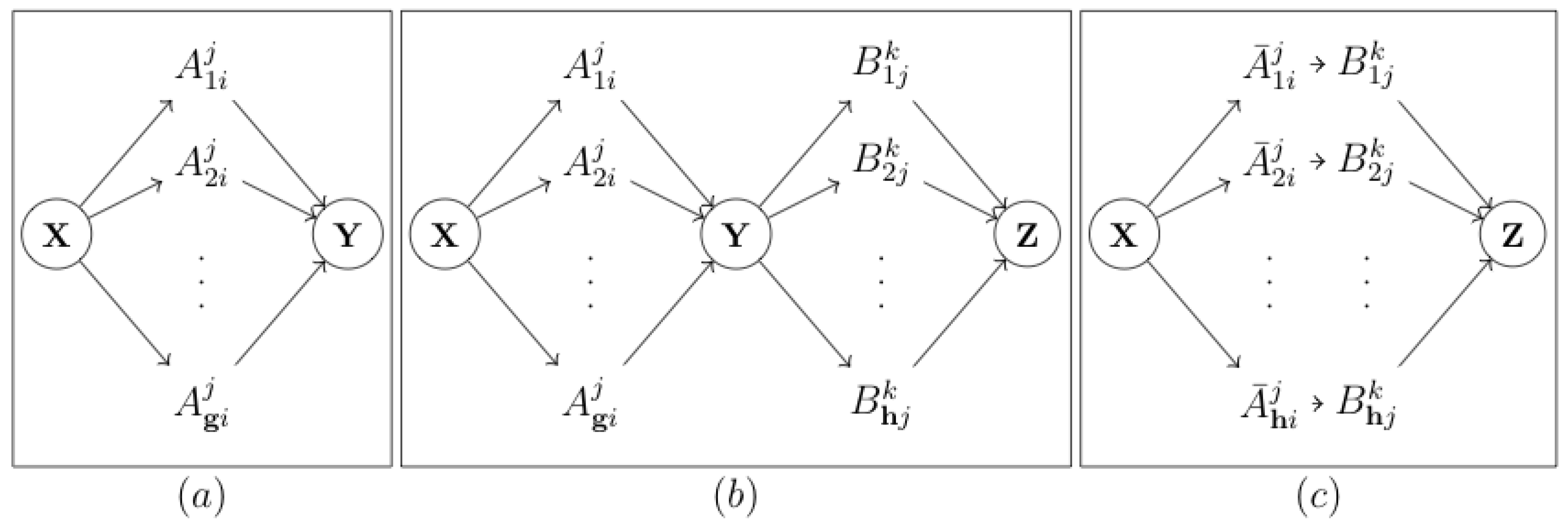
2.1.2. Tensor Representation of the Communication Channel
2.2. Transfer Entropy
2.2.1. The Causal Channel
2.2.2. The Chain
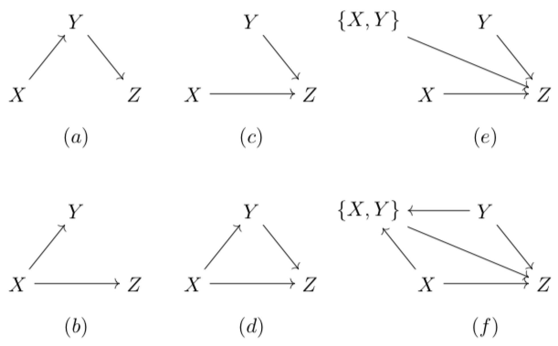
2.2.3. The Fork
2.2.4. The v-Structure and the Directed Triangle
3. Results
3.1. Differentiation Between Direct and Indirect Association using Bivariate Analysis
3.1.1. A Fork Can Be Differentiated from a Chain
3.1.2. Bivariate Analysis Suffices to Infer the Structure
3.1.3. A Directed Triangle Can Be Differentiated From a Chain and a Fork
3.1.4. A Data Processing Inequality Exists for TE
3.2. Examples
3.2.1. Differentiating Between Dyadic and Triadic Distributions
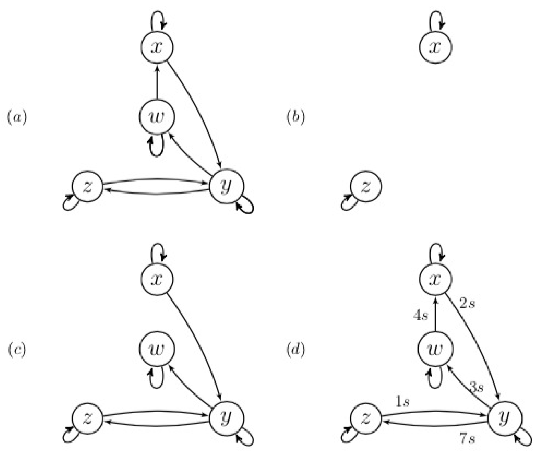
3.2.2. Coupled Ornstein–Uhlenbeck Processes
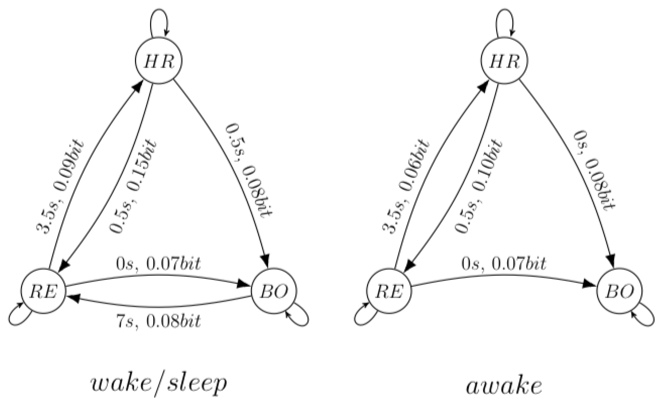
3.2.3. 1991 Santa Fe Time Series Competition Data Set B
4. Discussion
Funding
Acknowledgments
Conflicts of Interest
Abbreviations
| DMC | discrete memoryless communication channel |
| DPI | data processing inequality |
| MI | mutual information |
| pmf | probability mass function |
| TE | transfer entropy |
Appendix A. Overview and Proofs
Appendix A.1. Causal Channel
Appendix A.2. The Chain

Appendix A.3. Equivalence of a Fork and a Chain
Appendix A.4. The Interaction Tensor
Appendix A.5. Bivariate Analysis Suffices

Appendix A.6. The DPI
References
- Christensen, C.; Albert, R. Using Graph Concepts to Understand the Organization of Complex Systems. Int. J. Bifurc. Chaos 2007, 17, 2201–2214. [Google Scholar] [CrossRef]
- Guo, R.; Cheng, L.; Li, J.; Hahn, P.; Liu, H. A Survey of Learning Causality with Data: Problems and Methods. arXiv 2018, arXiv:1809.09337. [Google Scholar]
- Runge, J.; Heitzig, J.; Petoukhov, V.; Kurths, J. Escaping the Curse of Dimensionality in Estimating Multivariate Transfer Entropy. Phys. Rev. Lett. 2012, 108, 258701. [Google Scholar] [CrossRef] [PubMed]
- Pearl, J. Causality: Models, Reasoning and Inference, 2nd ed.; Cambridge University Press: New York, NY, USA, 2009. [Google Scholar]
- Eichler, M. Causal inference with multiple time series: Principles and problems. Philos. Trans. R. Soc. A 2013, 371, 20110613. [Google Scholar] [CrossRef] [PubMed]
- Margolin, A.; Nemenman, I.; Basso, K.; Wiggins, C.; Stolovitzky, G.; Dalla-Favera, R.; Califano, A. ARACNE: An Algorithm for the Reconstruction of Gene Regulatory Networks in a Mammalian Cellular Context. BMC Bioinform. 2006, 7, S7. [Google Scholar] [CrossRef]
- Vastano, J.A.; Swinney, H.L. Information transport in spatiotemporal systems. Phys. Rev. Lett. 1988, 60, 1773–1776. [Google Scholar] [CrossRef]
- Dagum, P.; Galper, A.; Horvitz, E. Dynamic Network Models for Forecasting. In Proceedings of the Eighth International Conference on Uncertainty in Artificial Intelligence (UAI’92), Stanford, CA, USA, 17–19 July 1992; Morgan Kaufmann Publishers Inc.: San Francisco, CA, USA, 1992; pp. 41–48. [Google Scholar]
- Spirtes, P.; Glymour, C.; Scheines, R. Causation, Prediction, and Search; MIT Press: Cambridge, MA, USA, 2000. [Google Scholar]
- Schreiber, T. Measuring Information Transfer. Phys. Rev. Lett. 2000, 85, 461–464. [Google Scholar] [CrossRef]
- Lizier, J.T.; Prokopenko, M. Differentiating information transfer and causal effect. Eur. Phys. J. B 2010, 73, 605–615. [Google Scholar] [CrossRef]
- Hyvärinen, A.; Zhang, K.; Shimizu, S.; Hoyer, P.O. Estimation of a Structural Vector Autoregression Model Using Non-Gaussianity. J. Mach. Learn. Res. 2010, 11, 1709–1731. [Google Scholar]
- Duan, P.; Yang, F.; Chen, T.; Shah, S. Direct Causality Detection via the Transfer Entropy Approach. IEEE Trans. Control Syst. Technol. 2013, 21, 2052–2066. [Google Scholar] [CrossRef]
- Sun, J.; Taylor, D.; Bollt, E. Causal Network Inference by Optimal Causation Entropy. SIAM J. Appl. Dyn. Syst. 2014, 14. [Google Scholar] [CrossRef]
- Turing, A.M. On Computable Numbers, with an Application to the Entscheidungsproblem. Proc. Lond. Math. Soc. 1937, s2-42, 230–265. [Google Scholar] [CrossRef]
- Ahmed, S.S.; Roy, S.; Kalita, J.K. Assessing the Effectiveness of Causality Inference Methods for Gene Regulatory Networks. IEEE/ACM Trans. Comput. Biol. Bioinform. 2018, 17, 56–70. [Google Scholar] [CrossRef] [PubMed]
- Rashidi, B.; Singh, D.S.; Zhao, Q. Data-driven root-cause fault diagnosis for multivariate non-linear processes. Control Eng. Pract. 2018, 70, 134–147. [Google Scholar] [CrossRef]
- Copeland, B.J. The Church-Turing Thesis. In the Stanford Encyclopedia of Philosophy, Spring 2019 ed.; Zalta, E.N., Ed.; Stanford University: Stanford, CA, USA, 2019. [Google Scholar]
- Shannon, C.E. A Mathematical Theory of Communication. Bell Labs Tech. J. 1948, 27, 379–423. [Google Scholar] [CrossRef]
- Cover, T.M.; Thomas, J.A. Elements of Information Theory; Wiley-Interscience: New York, NY, USA, 1991. [Google Scholar]
- Dullemond, K.; Peeters, K. Introduction to Tensor Calculus. 2010. Available online: https://www.semanticscholar.org/paper/Introduction-to-Tensor-Calculus-Dullemond-Peeters/5590e789439b21bede6cdd27517b99266d8255be (accessed on 26 March 2020).
- Papoulis, A.; Pillai, S.U. Probability, Random Variables, and Stochastic Processes, 4th ed.; McGraw Hill: New York, NY, USA, 2002. [Google Scholar]
- Dionisio, A.; Menezes, R.; Mendes, D. Mutual information: A measure of dependency for nonlinear time series. Physica A 2004, 344, 326–329. [Google Scholar] [CrossRef]
- Kundu, P.; Cohen, I.; Dowling, D. Cartesian Tensors. In Fluid Mechanics, 6th ed.; Academic Press: Cambridge, MA, USA, 2016; pp. 49–76. [Google Scholar] [CrossRef]
- Muroga, S. On the Capacity of a Discrete Channel. J. Phys. Soc. Jpn. 1953, 8, 484–494. [Google Scholar] [CrossRef]
- Beckenbach, E.F. Modern Mathematics for the Engineer: Second Series; McGraw-Hill: New York, NY, USA, 1961. [Google Scholar]
- Granger, C.W.J. Investigating Causal Relations by Econometric Models and Cross-Spectral Methods. Econometrica 1969, 37, 424–438. [Google Scholar] [CrossRef]
- Wibral, M.; Pampu, N.; Priesemann, V.; Siebenhühner, F.; Seiwert, H.; Lindner, M.; Lizier, J.T.; Vicente, R. Measuring information-transfer delays. PLoS ONE 2013. [Google Scholar] [CrossRef]
- Razak, F.; Jensen, H. Quantifying ’Causality’ in Complex Systems: Understanding Transfer Entropy. PLoS ONE 2014, 9, e99462. [Google Scholar]
- Dean, T. Network+ Guide to Networks, 6th ed.; Course Technology Press: Boston, MA, USA, 2012. [Google Scholar]
- Bell, M. On the commutativity of discrete memoryless channels in cascade. J Franklin Inst.-Eng. Appl. Math. 1993, 330, 1101–1111. [Google Scholar] [CrossRef]
- Berge, C. Graphs and Hypergraphs; Elsevier Science Ltd.: Oxford, UK, 1985. [Google Scholar]
- James, R.; Crutchfield, J. Multivariate Dependence Beyond Shannon Information. Entropy 2016, 19, 531. [Google Scholar] [CrossRef]
- Blahut, R. Computation of channel capacity and rate-distortion functions. IEEE Trans. Inform. Theory 1972, 18, 460–473. [Google Scholar] [CrossRef]
- Moser, S.M.; Chen, P.N.; Lin, H.Y. Error Probability Analysis of Binary Asymmetric Channels. 2010. Available online: https://moser-isi.ethz.ch/docs/papers/smos-2010-2.pdf (accessed on 26 March 2020).
- Brown, L.D.; Cai, T.T.; DasGupta, A. Interval Estimation for a Binomial Proportion. Stat. Sci. 2001, 16, 101–133. [Google Scholar]
- Rigney, D.F.; Goldberger, A.L.; Ocasio, W.C.; Ichimaru, Y.; Moody, G.B.; Mark, R.G. Multi-channel physiological data: Description and analysis. In Time Series Prediction: Forecasting the Future and Understanding the Past; Weigend, A.S., Gershenfeld, N.A., Eds.; Addison-Wesley: Reading, MA, USA, 1993; pp. 105–129. [Google Scholar]
- Goldberger, A.L.; Amaral, L.A.; Glass, L.; Hausdorff, J.M.; Ivanov, P.C.; Mark, R.G.; Mietus, J.E.; Moody, G.B.; Peng, C.K.; Stanley, H.E. PhysioBank, PhysioToolkit, and PhysioNet: Components of a new research resource for complex physiologic signals. Circulation 2003, 101, e215–e220. [Google Scholar] [CrossRef]
- Williams, P.L.; Beer, R.D. Nonnegative Decomposition of Multivariate Information. arXiv 2010, arXiv:1004.2515. [Google Scholar]


| Process | Variable | Alphabet Element | Index (Input) | Index (Past) | Index (Output) |
|---|---|---|---|---|---|
| X | x | f | i | ||
| Y | y | g | j | ||
| Z | z | h | k |
| (a) Dyadic | (b) Triadic | ||||||
|---|---|---|---|---|---|---|---|
| X | Y | Z | p | X | Y | Z | p |
| 0 | 0 | 0 | 0 | 0 | 0 | ||
| 0 | 2 | 1 | 1 | 1 | 1 | ||
| 1 | 0 | 2 | 0 | 2 | 2 | ||
| 1 | 2 | 3 | 1 | 3 | 3 | ||
| 2 | 1 | 0 | 2 | 0 | 2 | ||
| 2 | 3 | 1 | 3 | 1 | 3 | ||
| 3 | 1 | 2 | 2 | 2 | 0 | ||
| 3 | 3 | 3 | 3 | 3 | 1 | ||
© 2020 by the author. Licensee MDPI, Basel, Switzerland. This article is an open access article distributed under the terms and conditions of the Creative Commons Attribution (CC BY) license (http://creativecommons.org/licenses/by/4.0/).
Share and Cite
Sigtermans, D. Towards a Framework for Observational Causality from Time Series: When Shannon Meets Turing. Entropy 2020, 22, 426. https://doi.org/10.3390/e22040426
Sigtermans D. Towards a Framework for Observational Causality from Time Series: When Shannon Meets Turing. Entropy. 2020; 22(4):426. https://doi.org/10.3390/e22040426
Chicago/Turabian StyleSigtermans, David. 2020. "Towards a Framework for Observational Causality from Time Series: When Shannon Meets Turing" Entropy 22, no. 4: 426. https://doi.org/10.3390/e22040426
APA StyleSigtermans, D. (2020). Towards a Framework for Observational Causality from Time Series: When Shannon Meets Turing. Entropy, 22(4), 426. https://doi.org/10.3390/e22040426