Gaussian Curvature Entropy for Curved Surface Shape Generation

Abstract
1. Introduction
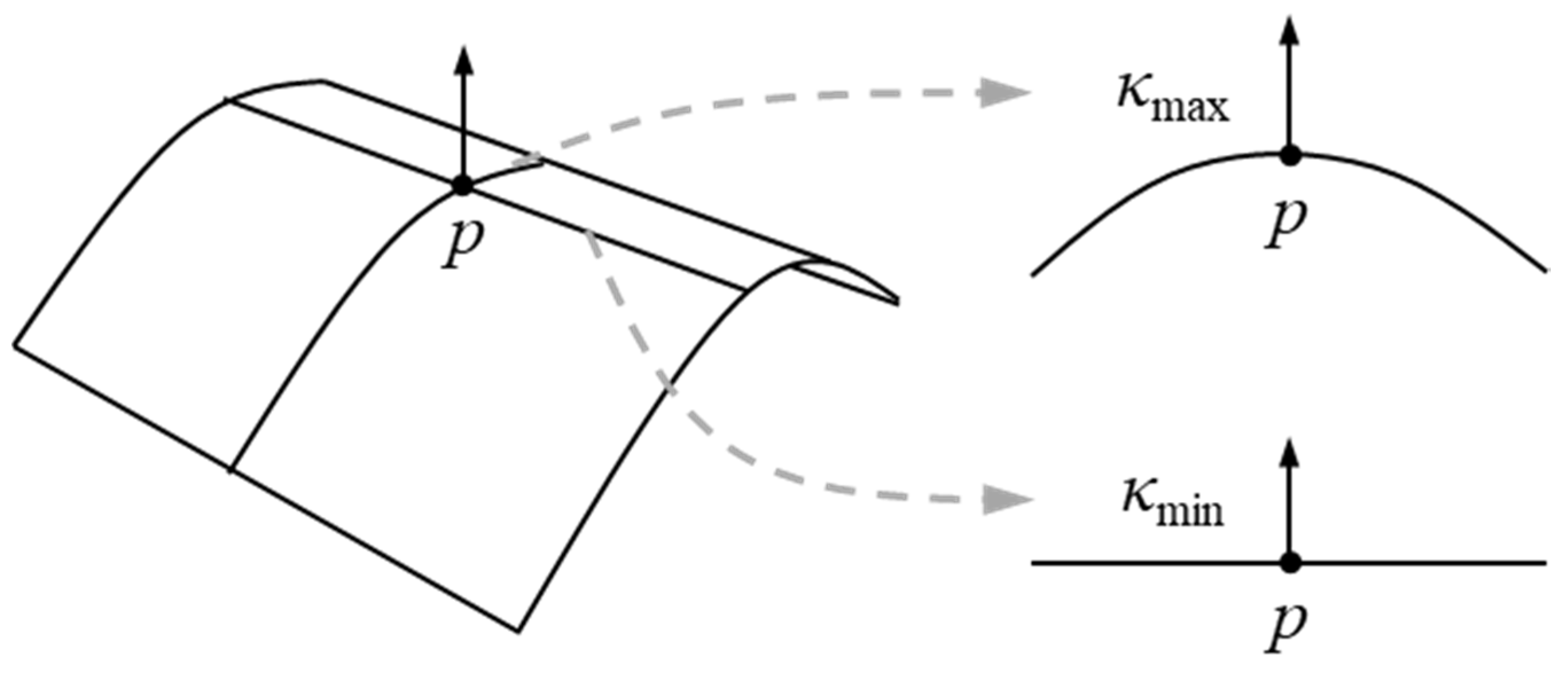
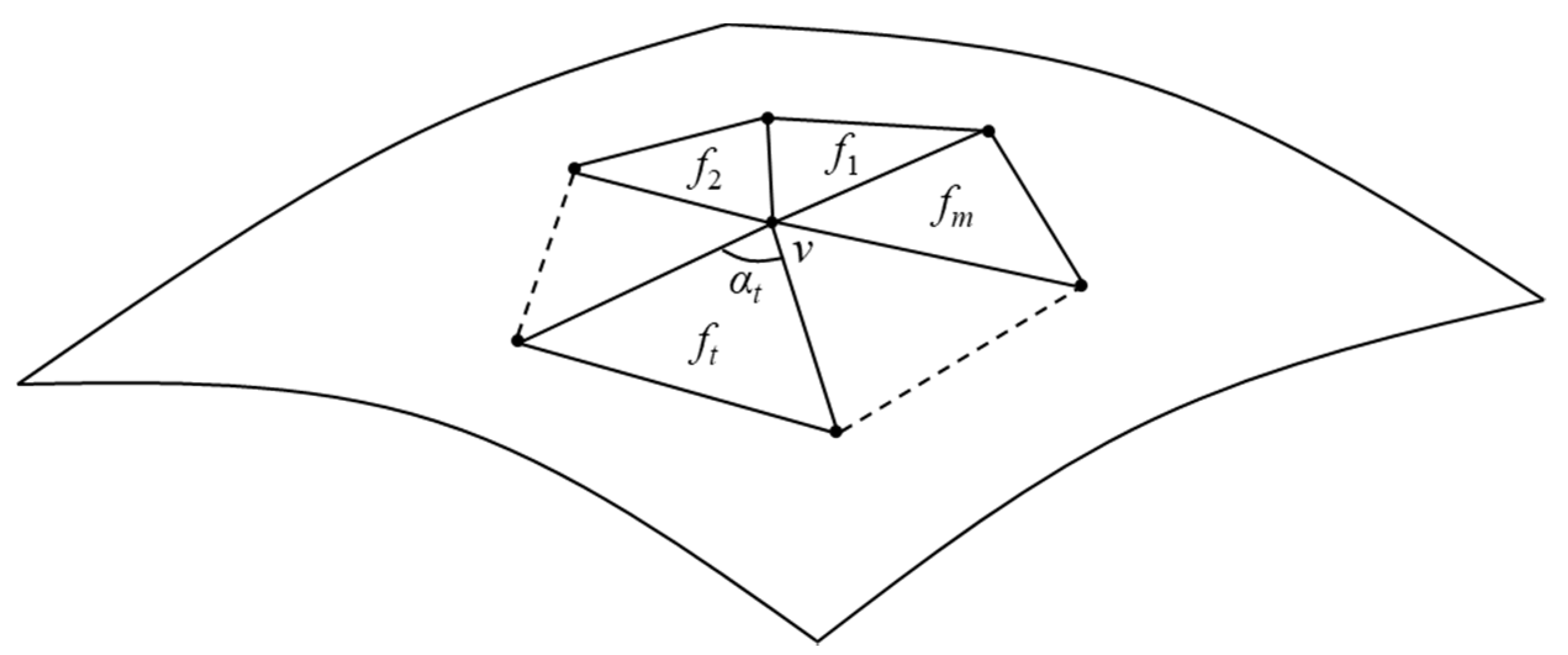
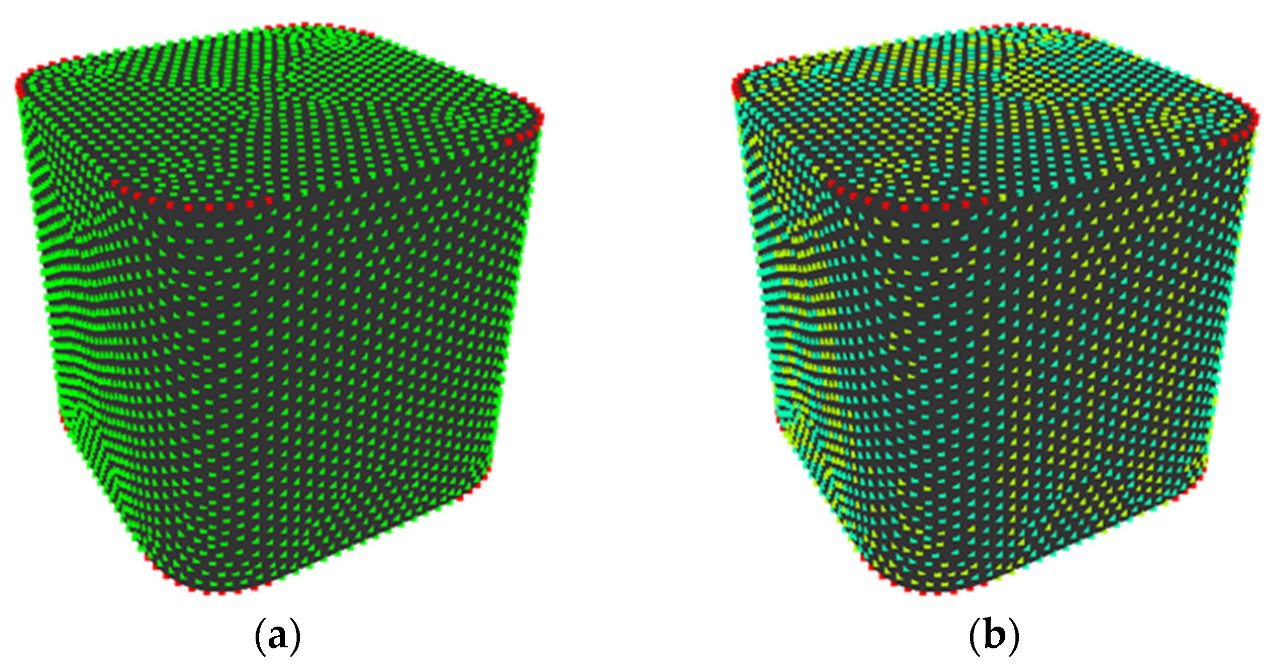
2. Gaussian Curvature Entropy
2.1. Construction of Gaussian Curvature Entropy
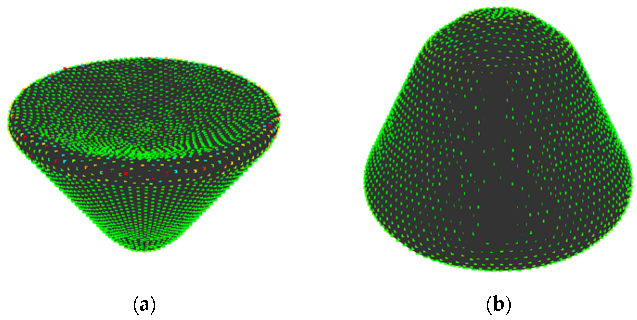
2.2. Experiment for Validation of Gaussian Curvature Entropy
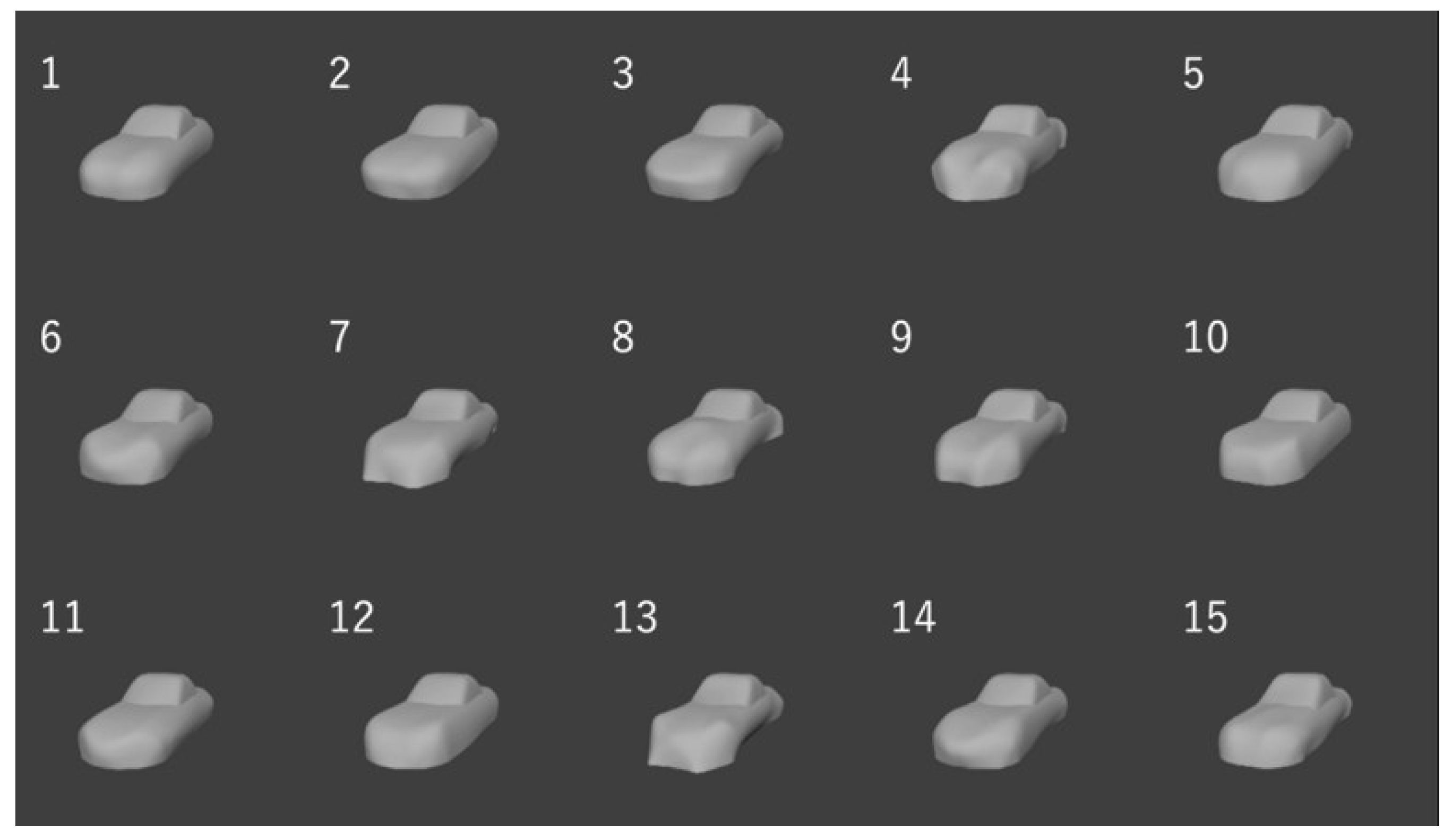
2.2.1. Experimental Methods
- Evaluation method: This experiment adopts a five-point Likert scale (1: “not complex”, 2: “slightly complex”, 3: “fairly complex”, 4: “complex”, and 5: “very complex”) to obtain sensory evaluation values about complexity in samples shapes.
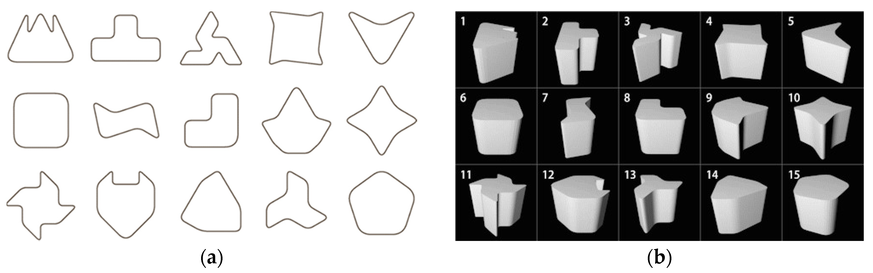
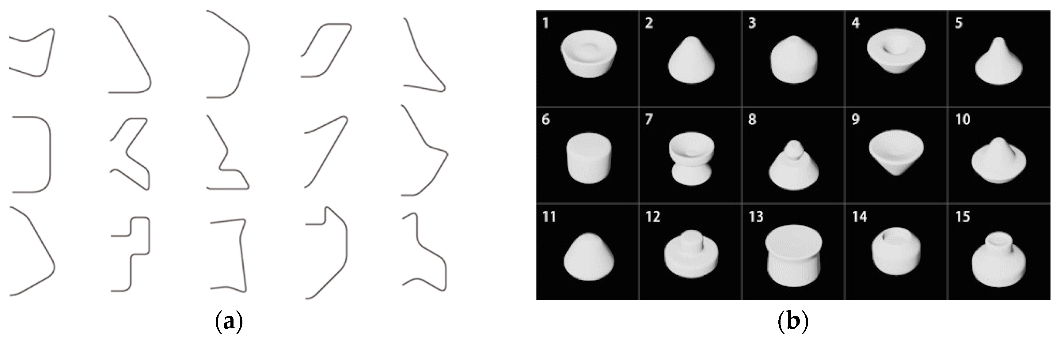
- Sample shapes displaying method: White sample shapes on a black background are simultaneously displayed on a seven-inch tablet device. During the experiment, these shapes are rotated at a constant speed (x axis: 0 rpm, y axis: 0 rpm, z axis: 12 rpm) with the center of gravity as the axis, so that the appearance of all concavities can be observed.
- Presentation method: The distance between the eyeball of a participant and the device was set to 500 mm. 15 sample shapes on the display simultaneously enter the field of view.
- Participant: 30 participants (23 men and seven women), ranging in age from 18 to 54 years (M = 25.5, SD = 7.78).
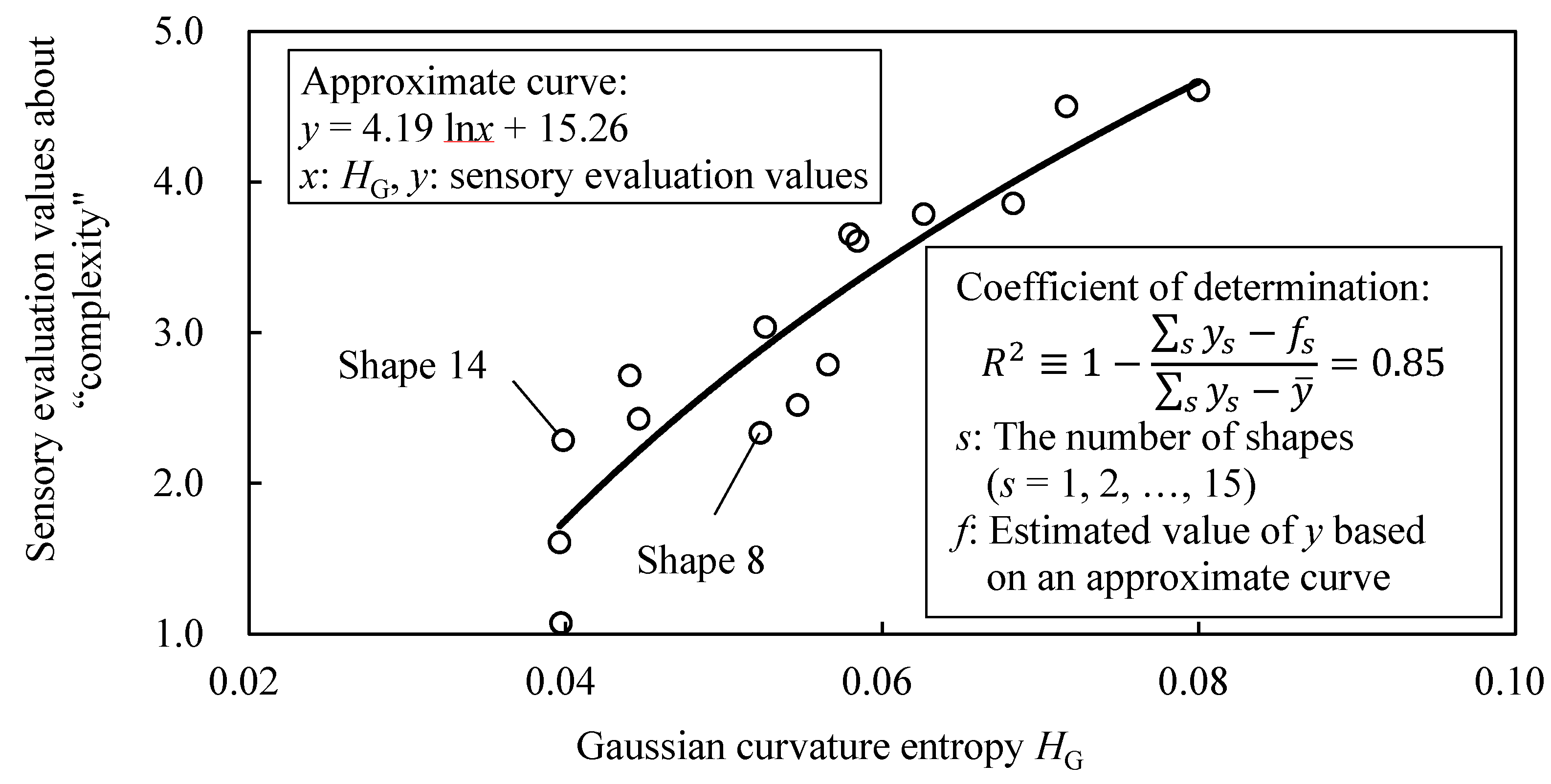
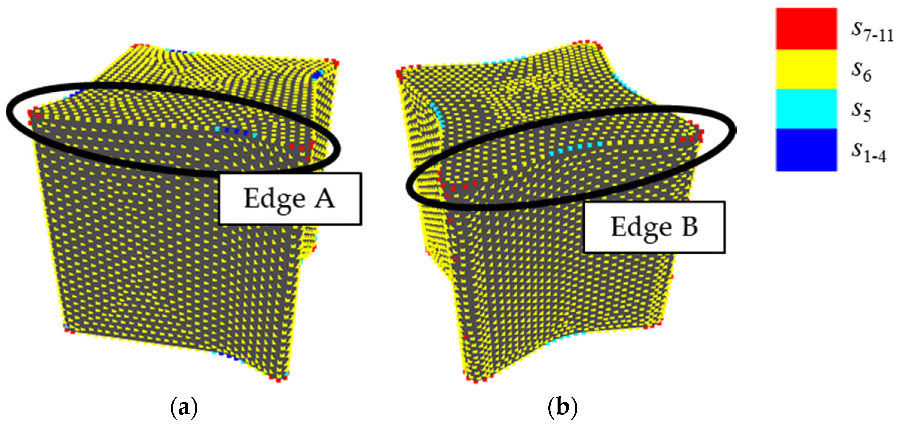
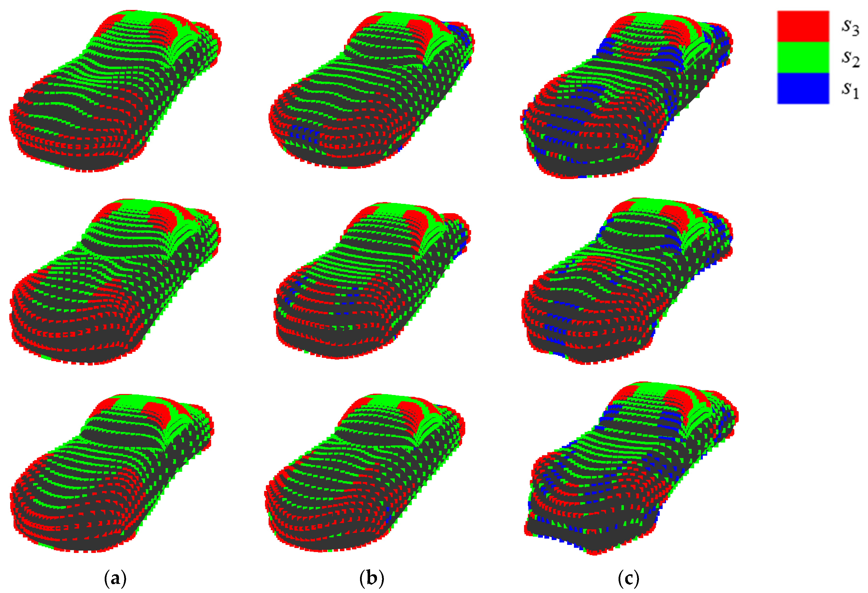
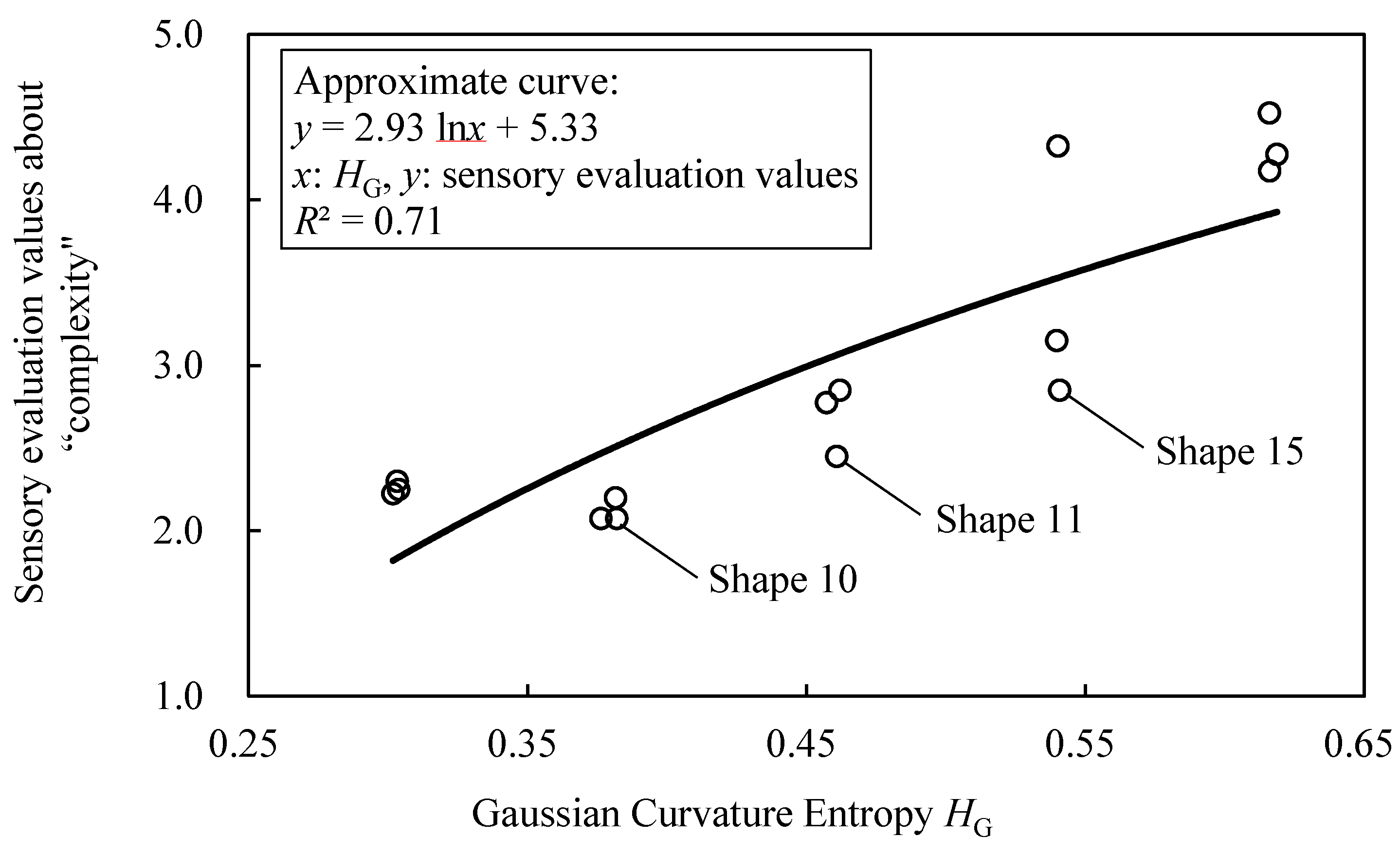
2.2.2. Experimental Results and Discussion
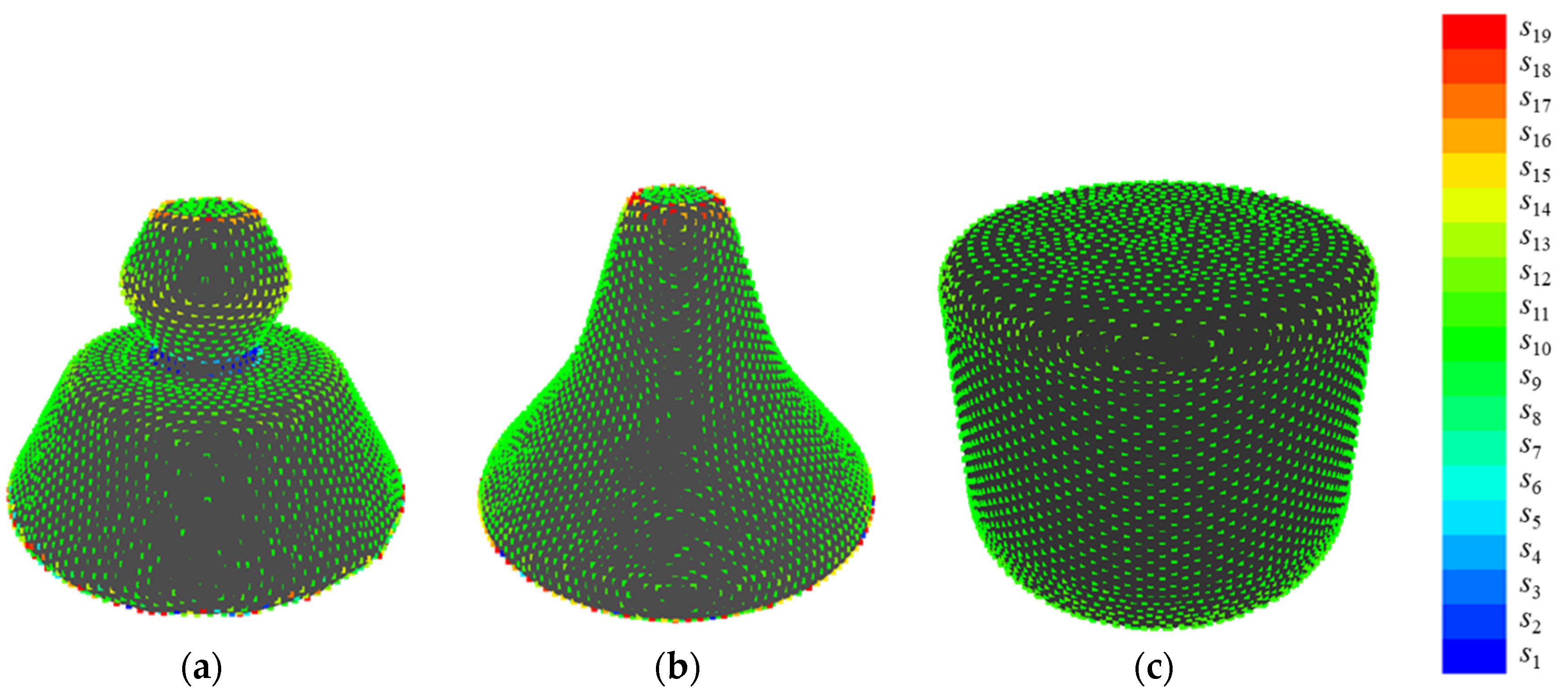
3. Shape Generation Method
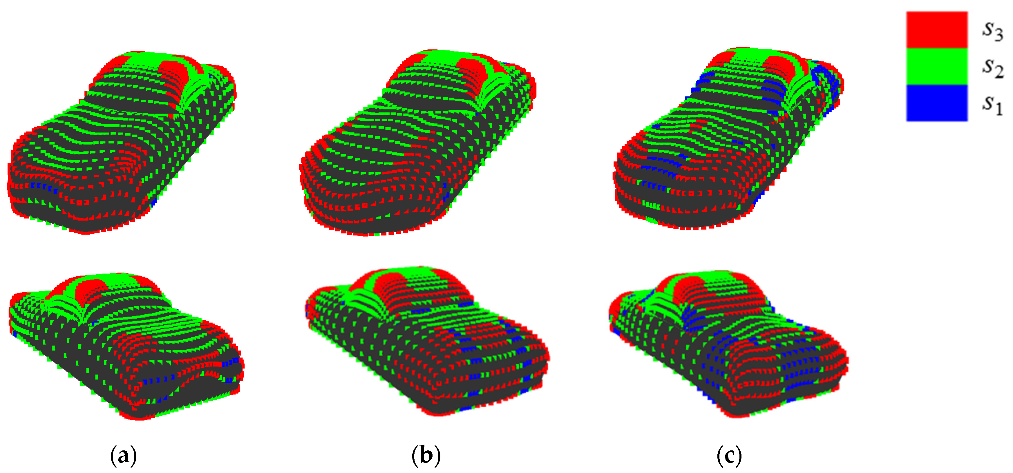
3.1. Construction of Shape Generation Method
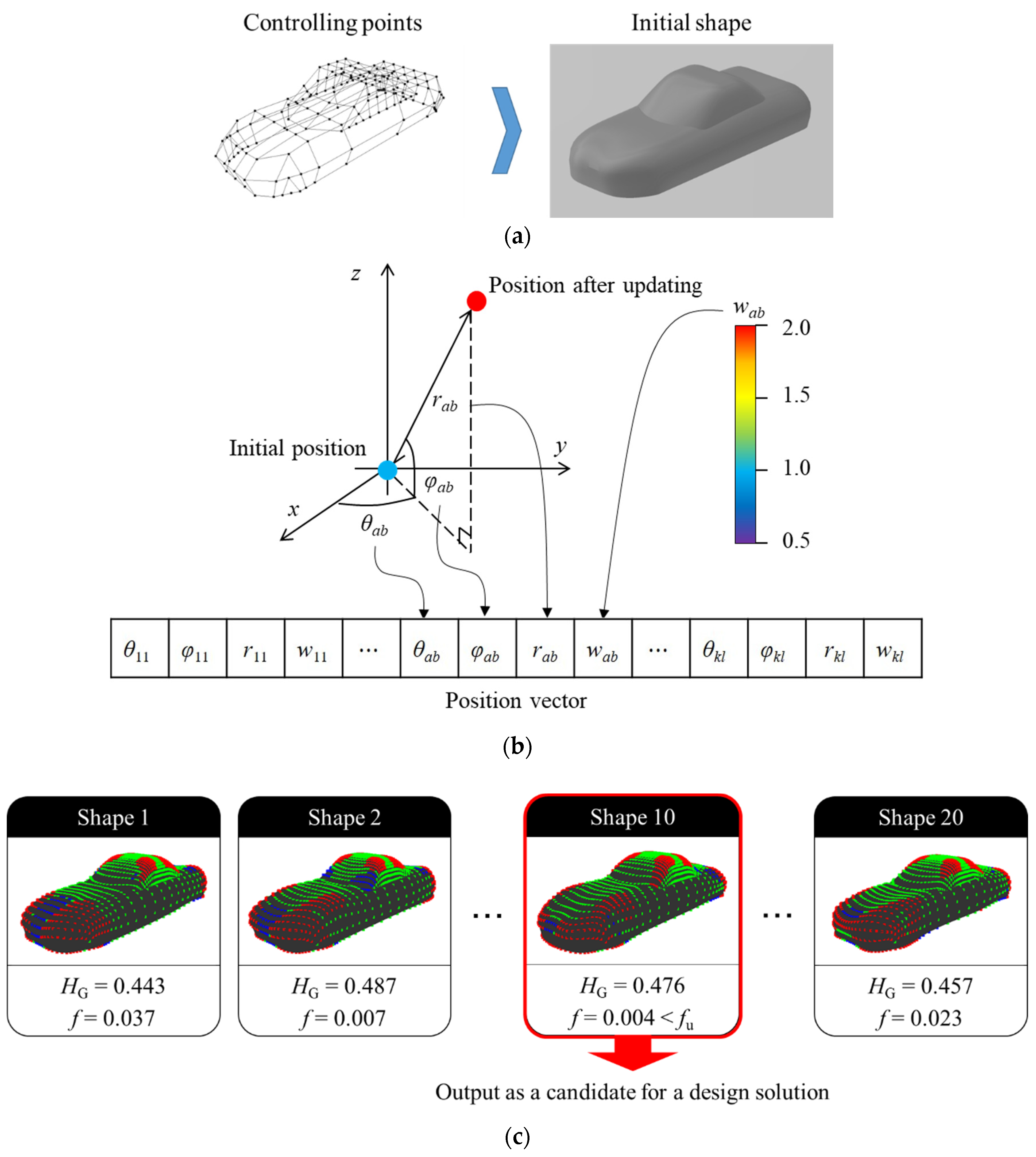
- (i)
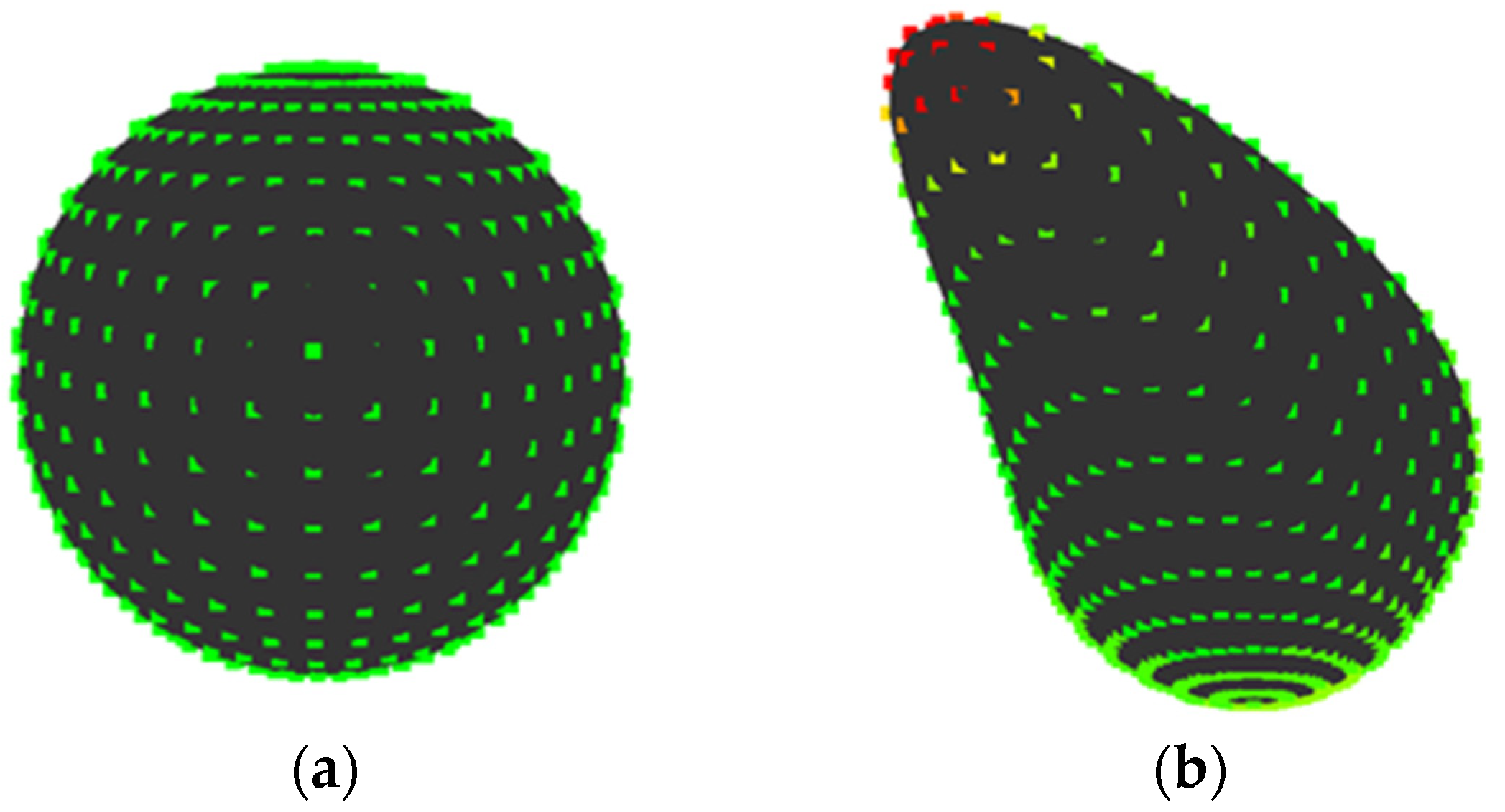
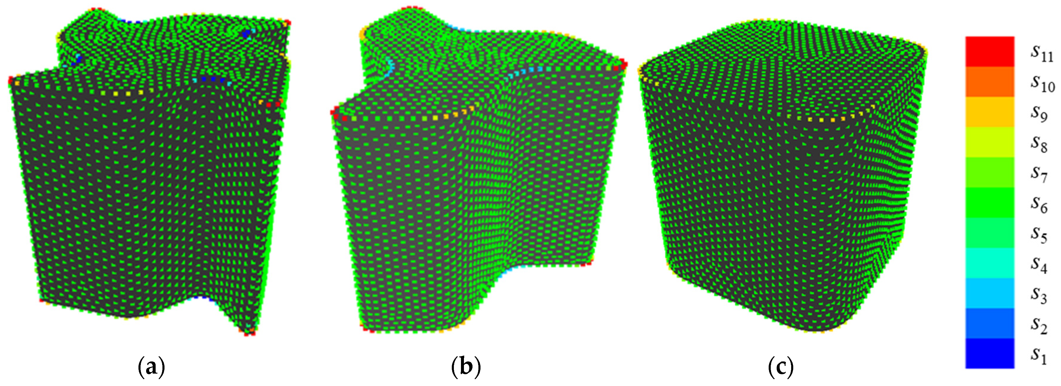
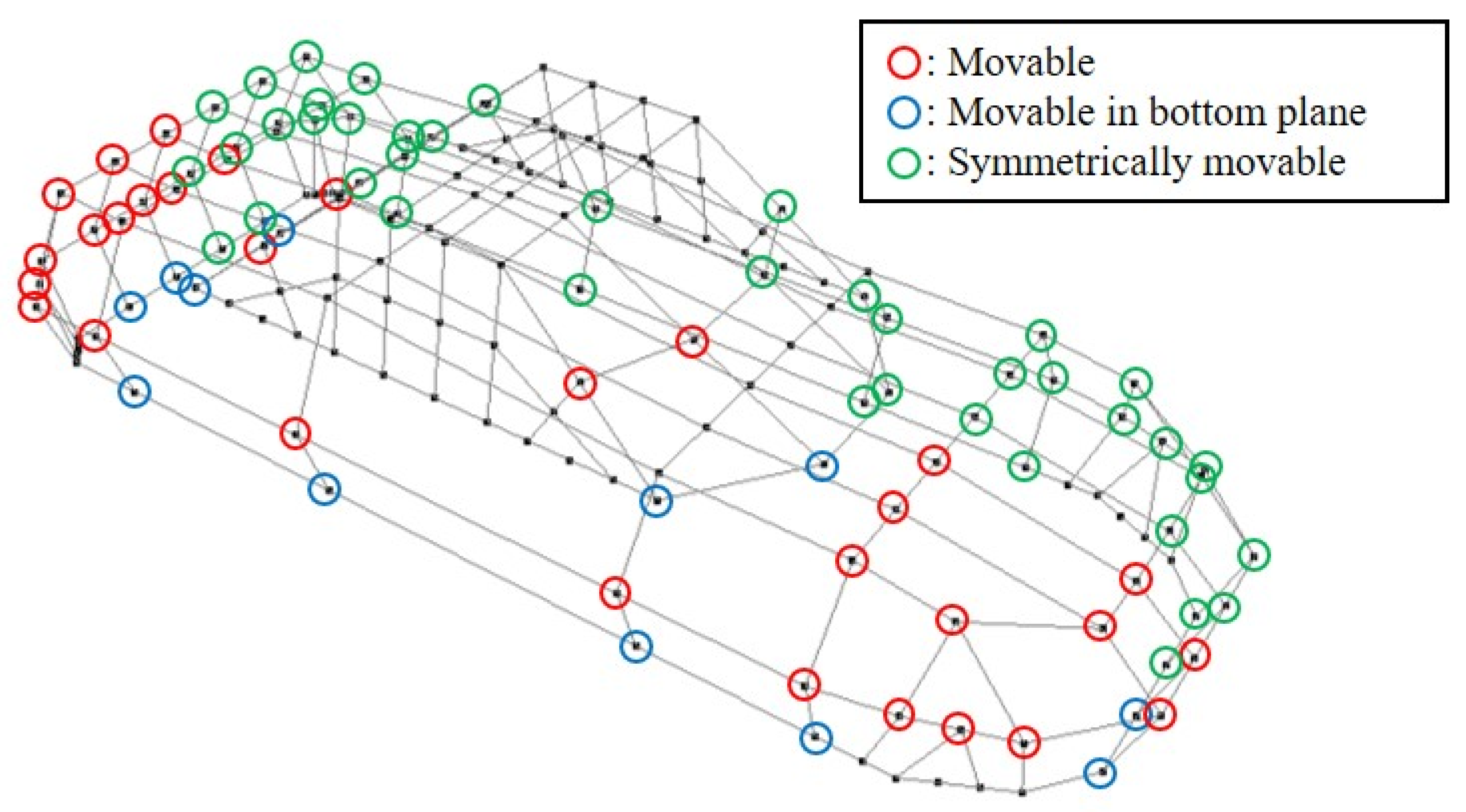
- Set the initial shape (Figure 19a). Subsequently, the initial shape is expressed while using the NURBS surface and Qab and wab of the surface is defined as the position vectors of particles in PSO (Figure 19b). Note that Qab is expressed by polar coordinates whose origin is the position of the controlling point at the initial shape.
- (ii)
- Set HG,target (targeted value of HG) and fu (allowable difference between HG and HG,target) as a condition of a candidate for solution.
- (iii)
- Generate shapes that are based on a position vector of particles renewed by movement of particles. Subsequently, HG and fitness f of the shapes is calculated. Note that the movable range of rab during movement is the half of the distance to the closest controlling point. In addition, this research set the range of wab to 0.5 ≤ wab ≤ 2.0, since the shape transforms drastically by changing the value in the range. Finally, if f of a generated shape is lower than fu, the shape is output as a candidate for solution. On the other hand, the movement of particles generates other shapes if there are no shapes meeting the condition.
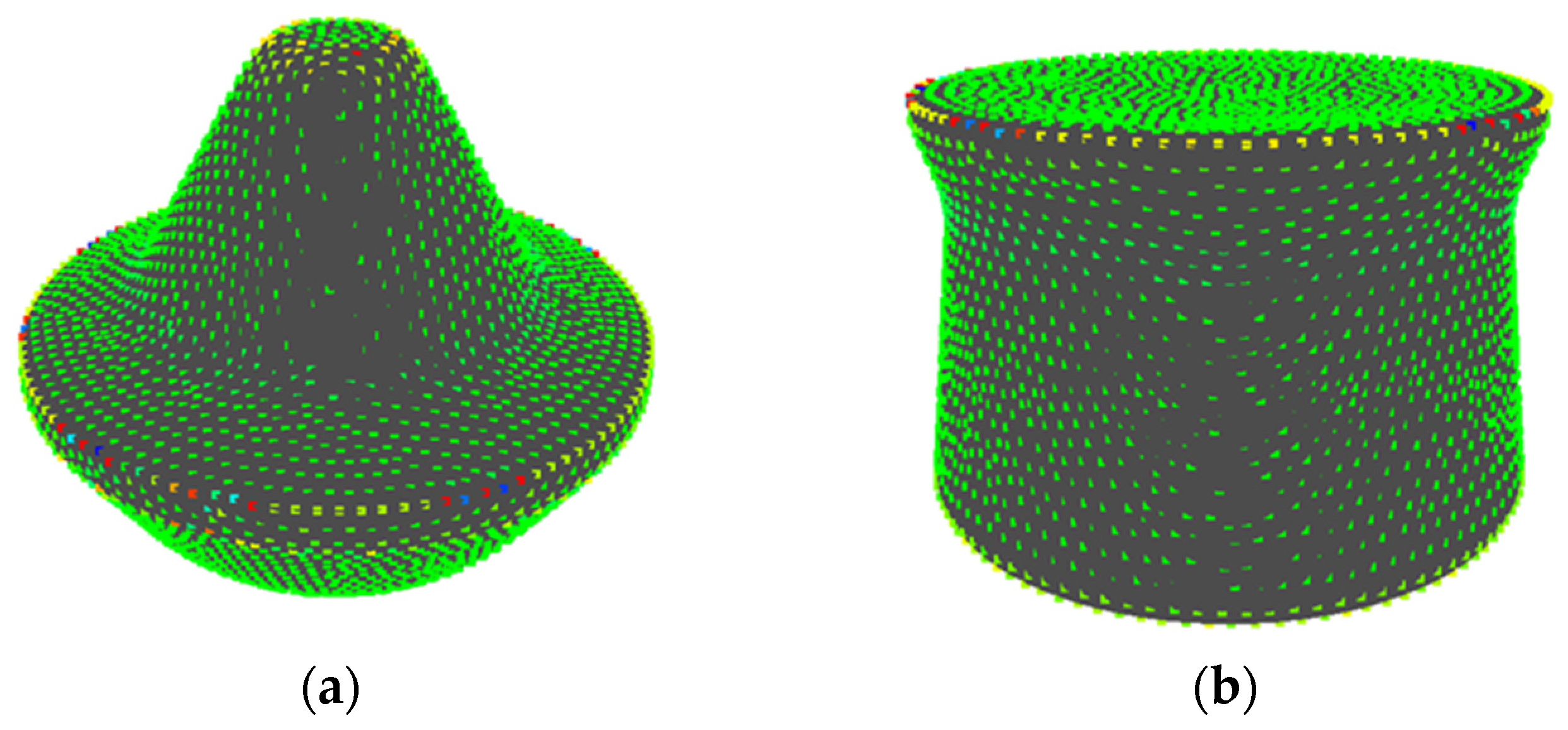
3.2. Experiment for Validation of Shape Generation Method
3.2.1. Experimental Methods
- Evaluation method: Just the same as Section 2.2.1.
- Sample shapes displaying method: White generated shapes on a black background were simultaneously displayed on a 13.3-inch laptop computer (Figure 22). During the experiment, each shape is rotated at a constant speed (x axis: 0 rpm, y axis: 0 rpm, z axis: 10 rpm), so that the appearance of all concavities can be observed.
- Presentation method: The distance between the eyeball of a participant and the computer was set to 500 mm. 15 sample shapes on the display simultaneously enter the field of view.
- Participants: 40 participants (36 men and four women) that ranged in age from 16 to 61 years (M = 23.9, SD = 7.67).
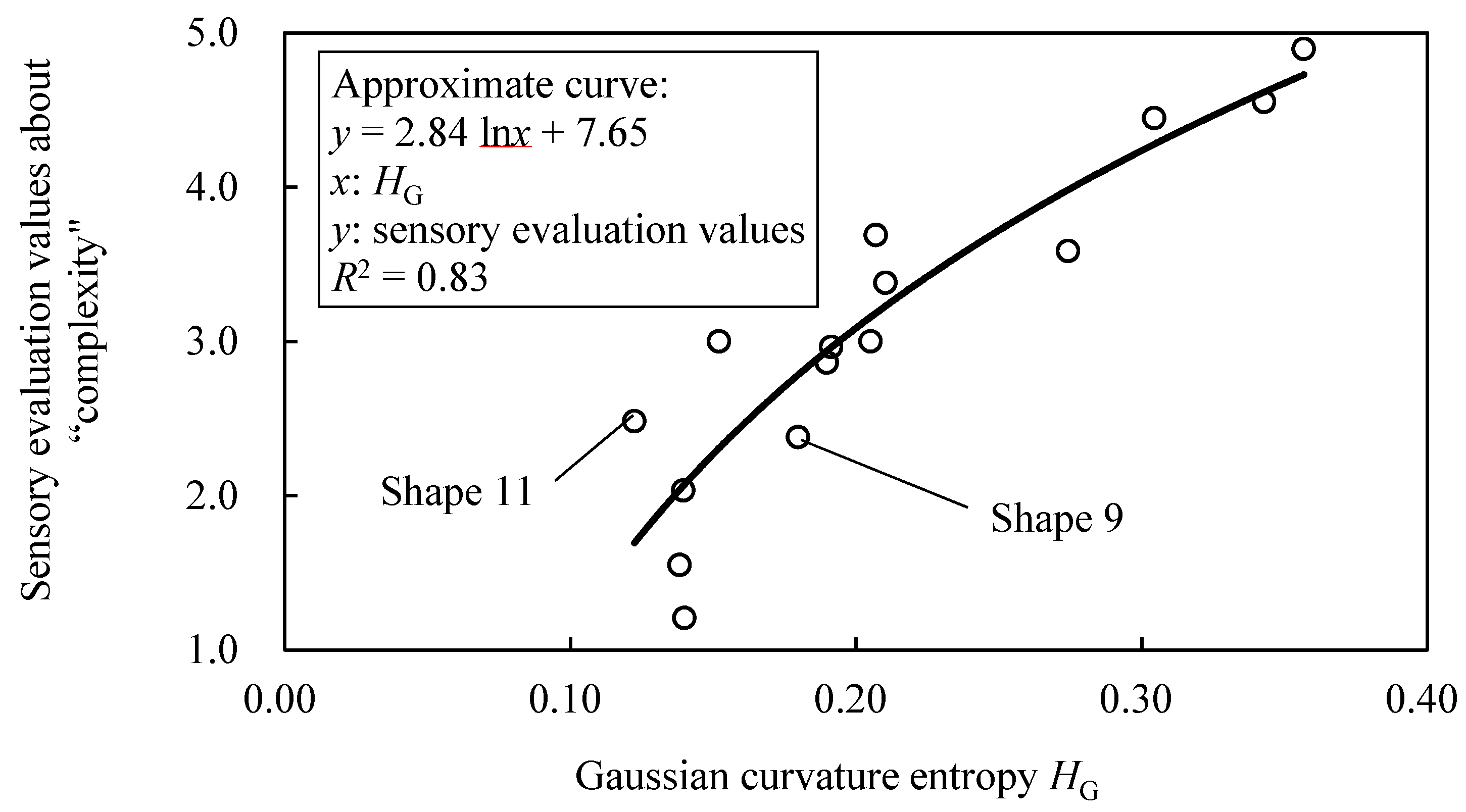
3.2.2. Experimental Results and Discussion
4. Conclusions
Author Contributions
Funding
Conflicts of Interest
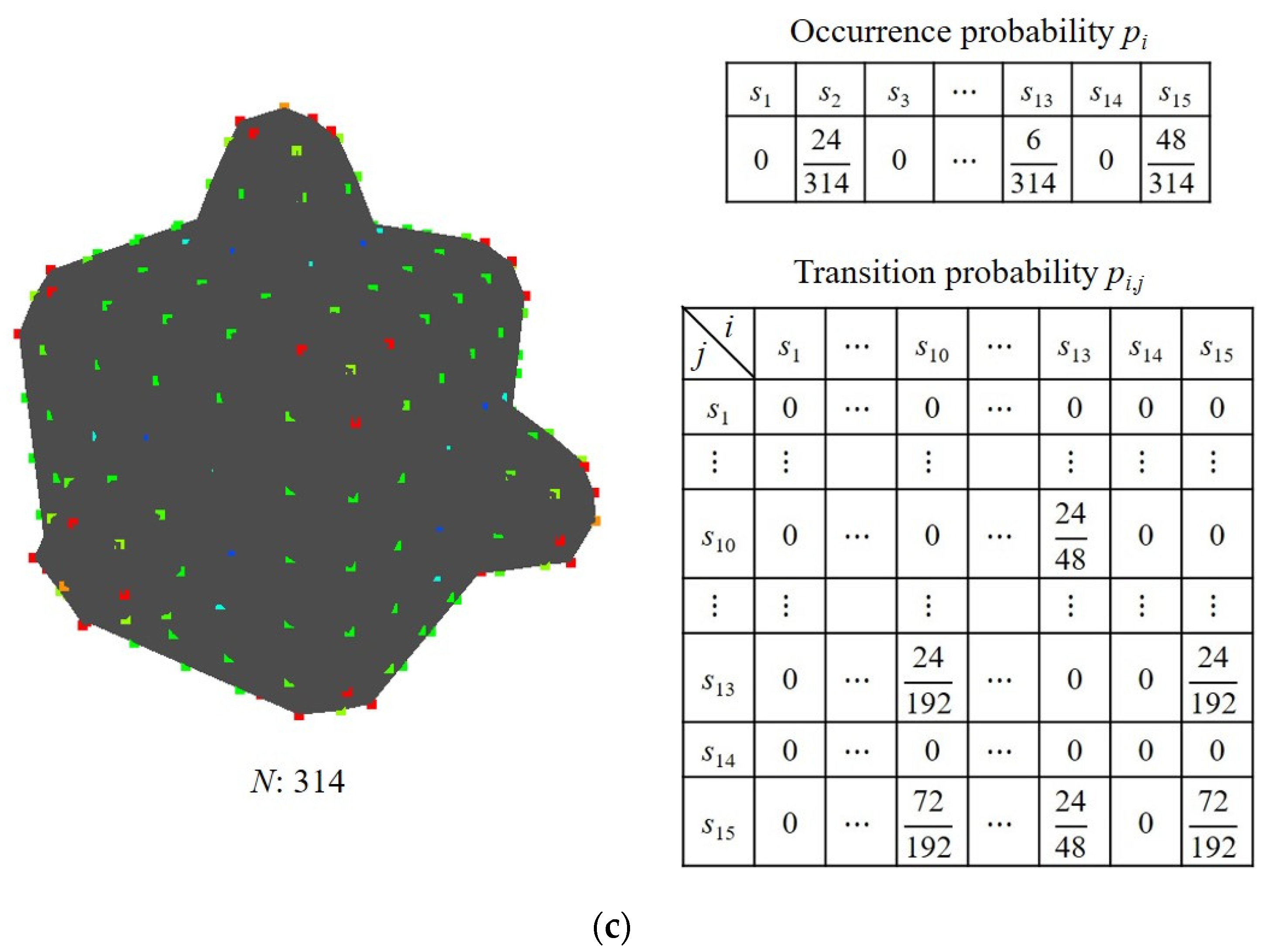
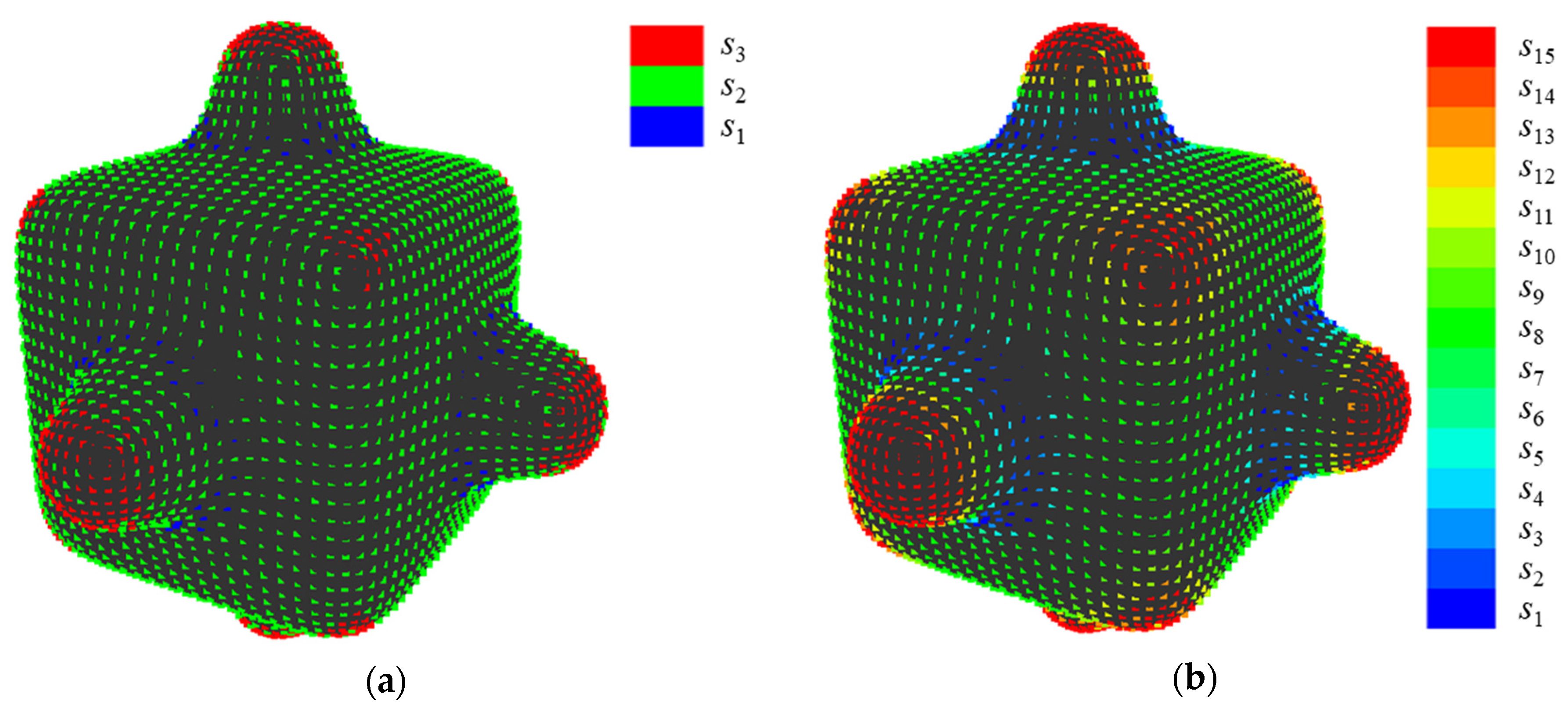
Appendix A
Appendix B
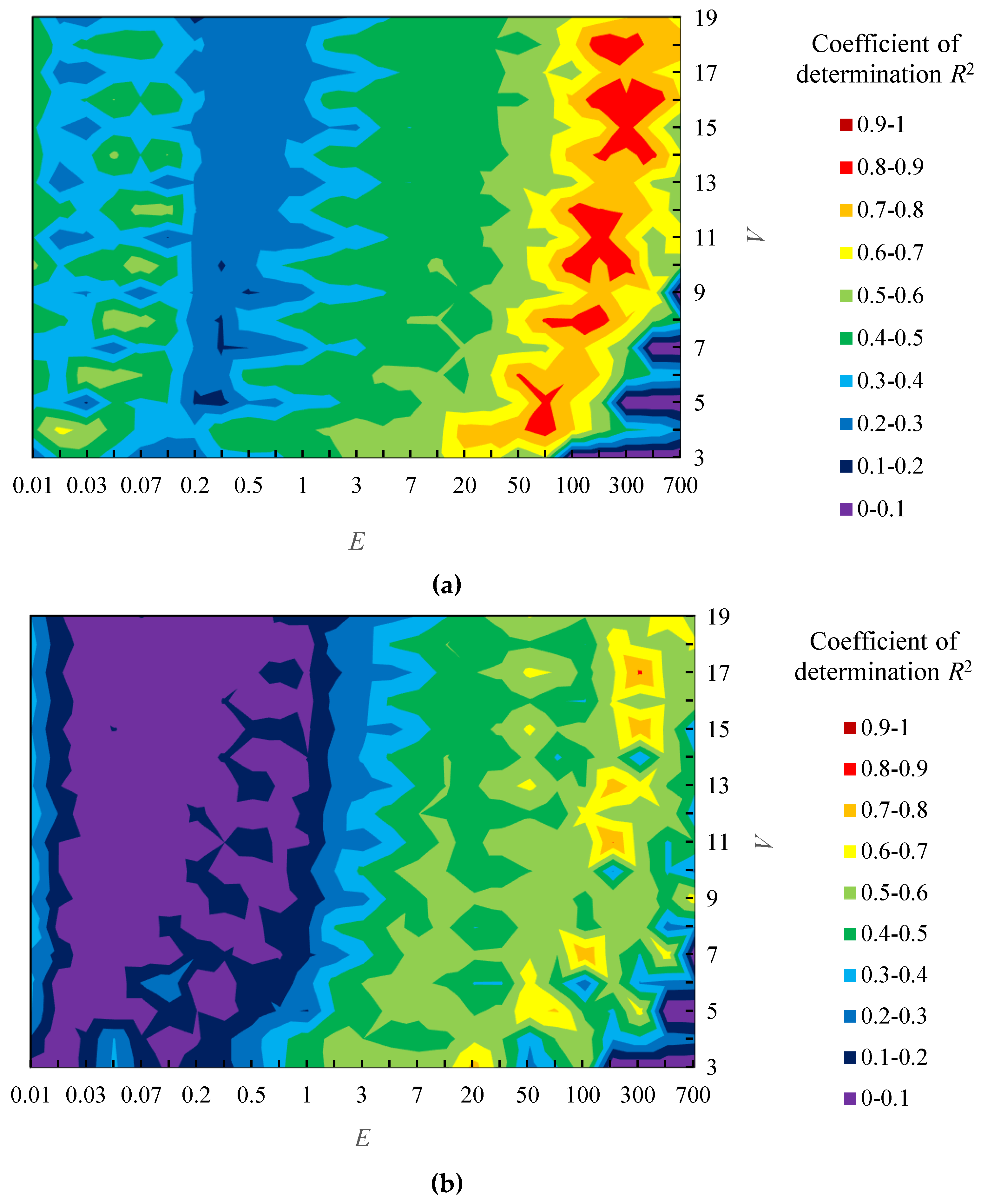
- (i)
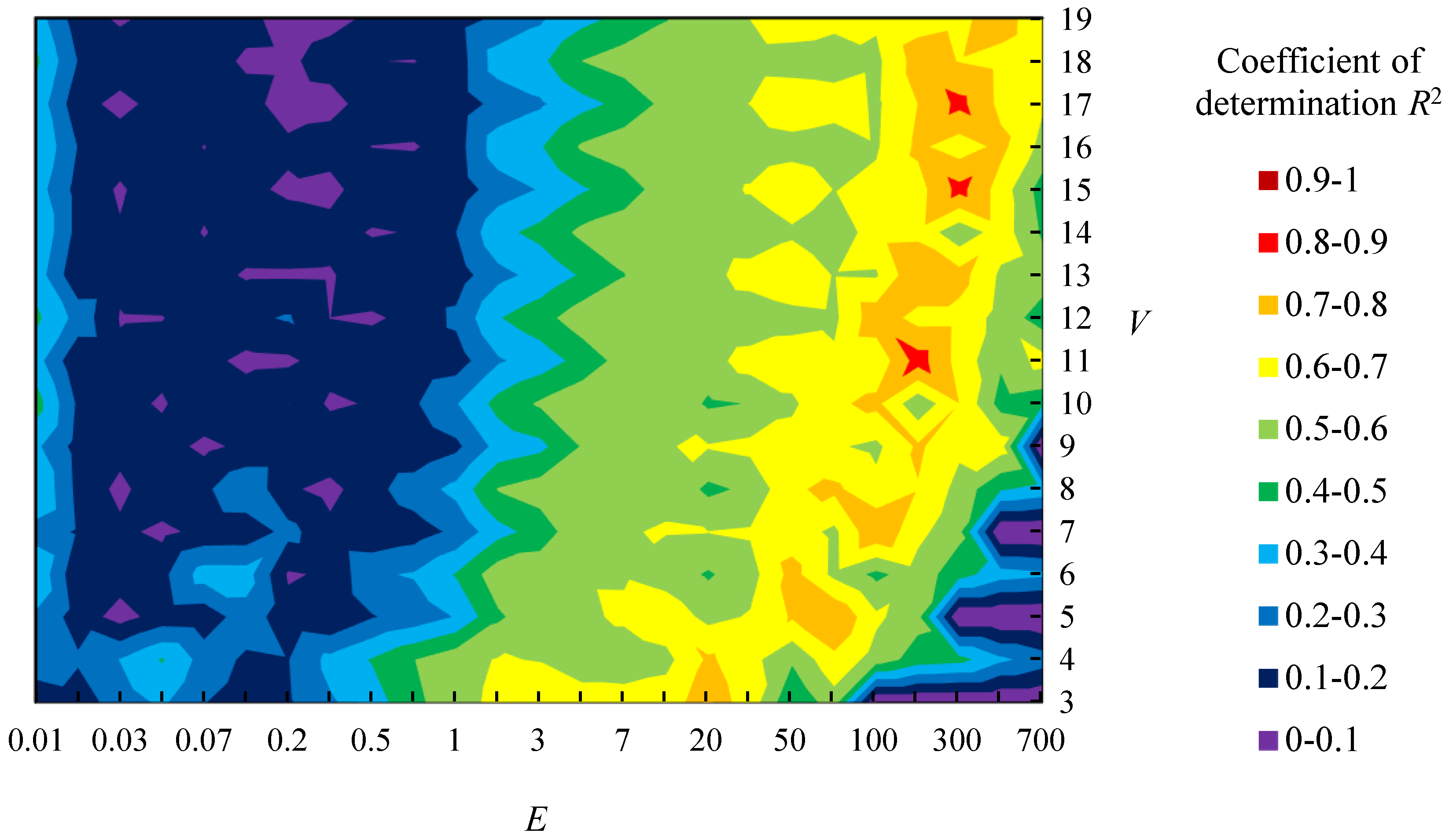
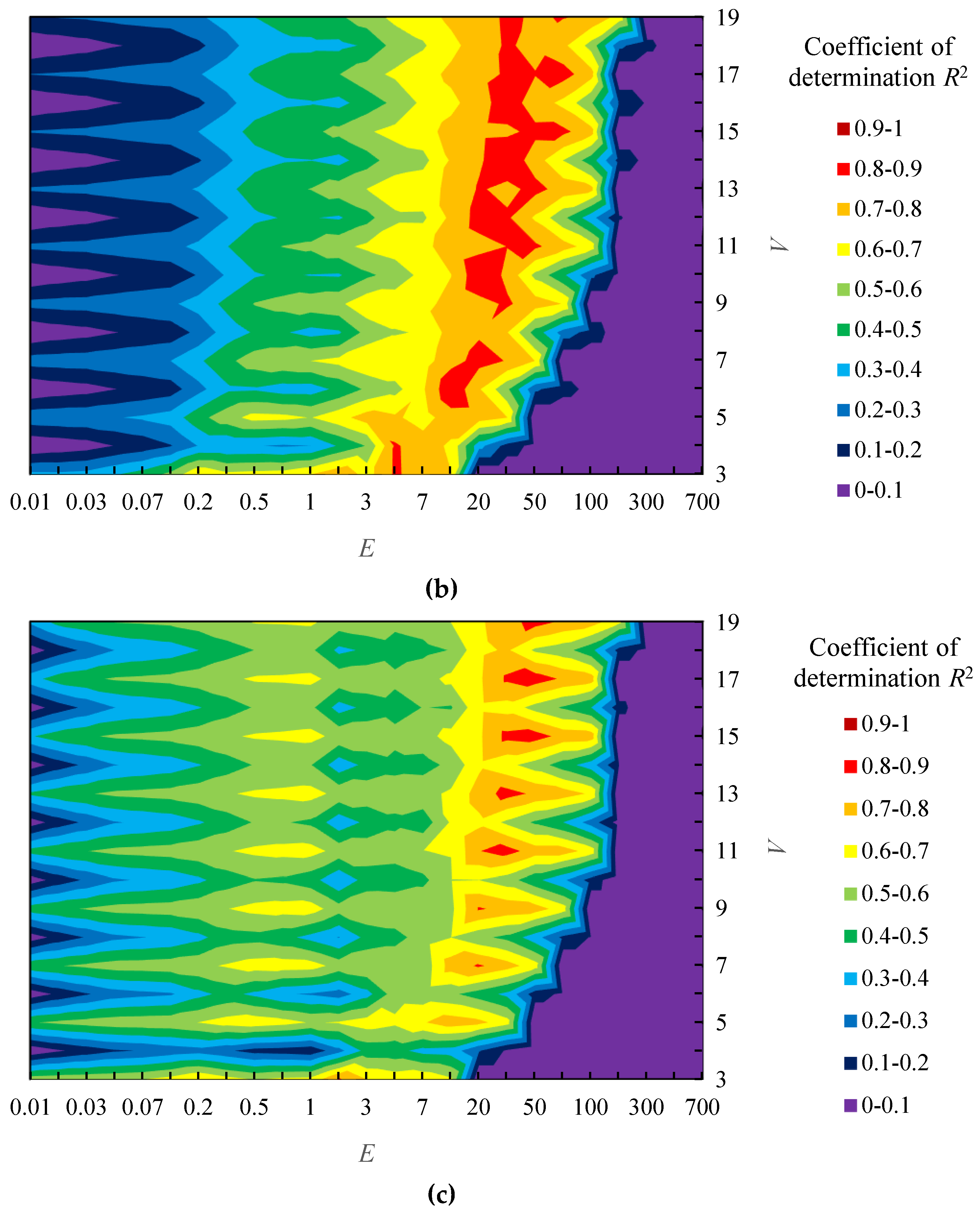
- Divide sample shapes A into 3 groups (Group A1, A2 and A3). In order to ensure that each group includes shapes with various sensory evaluation values about “complexity”, the shapes are assigned to the group based on the sensory evaluation values. In particular, 15 shapes were sorted in descending order of the sensory evaluation values and 5 categories were made by selecting 3 shapes in the order. Then, one shape was randomly selected from each category and 3 groups were made for the cross-validation.
- (ii)
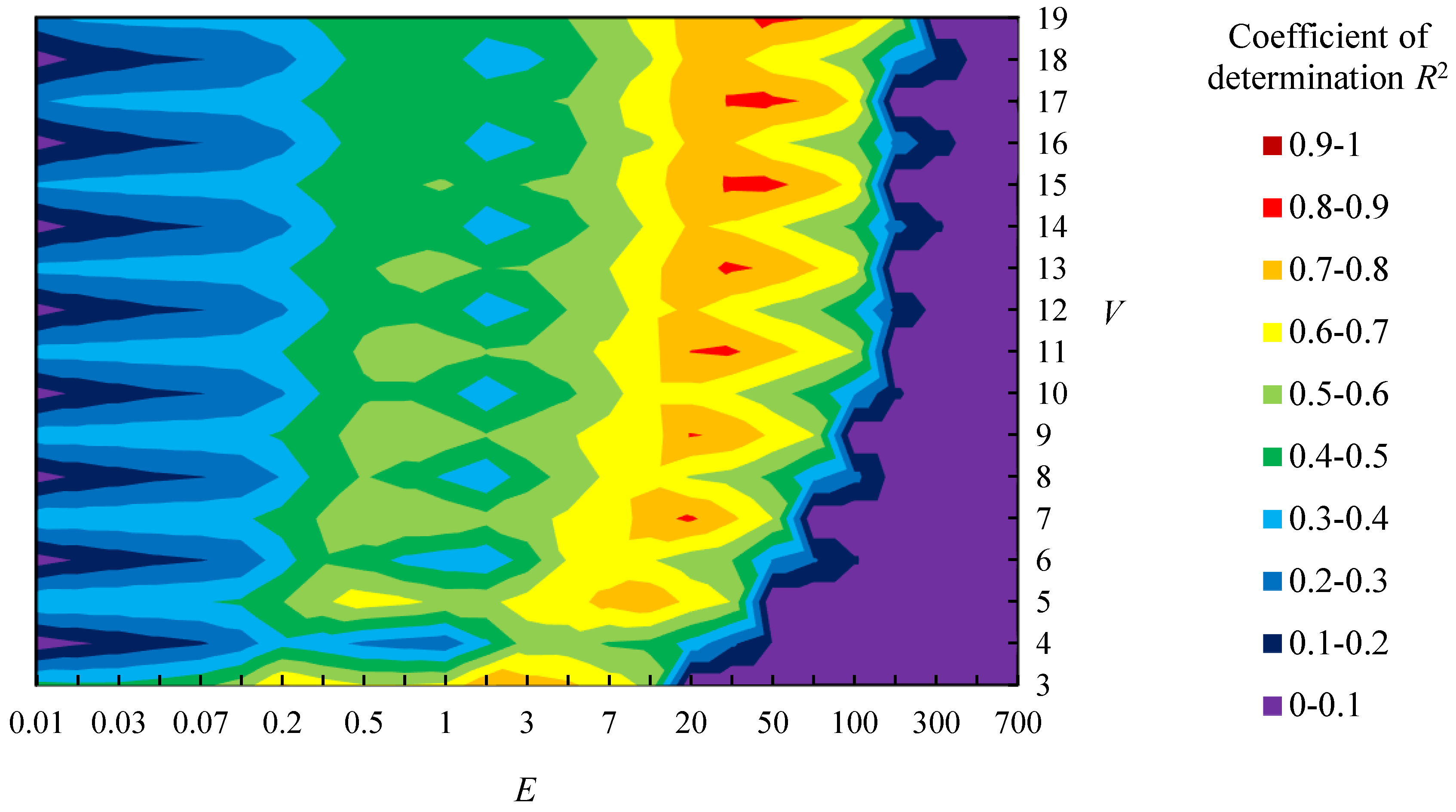
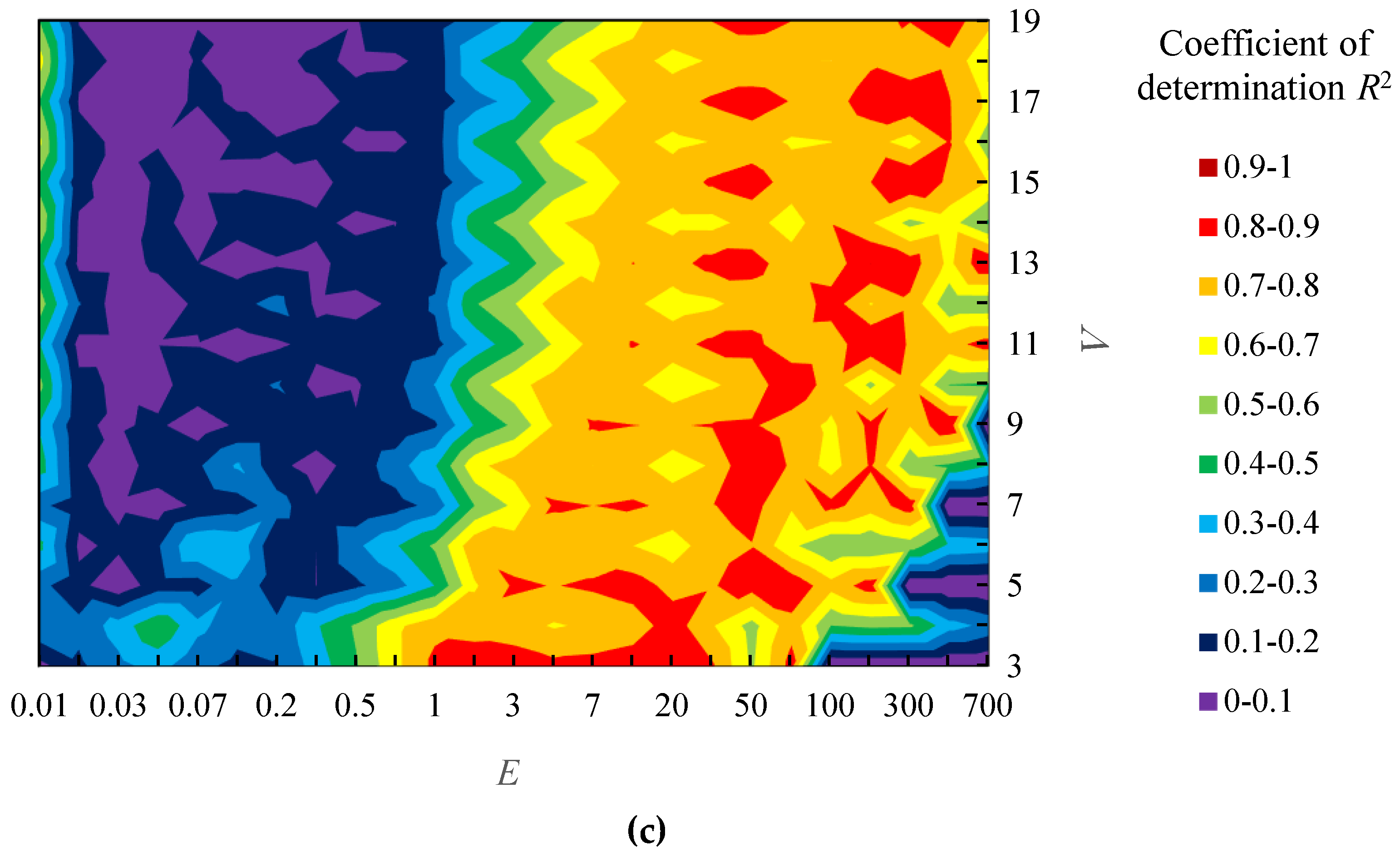
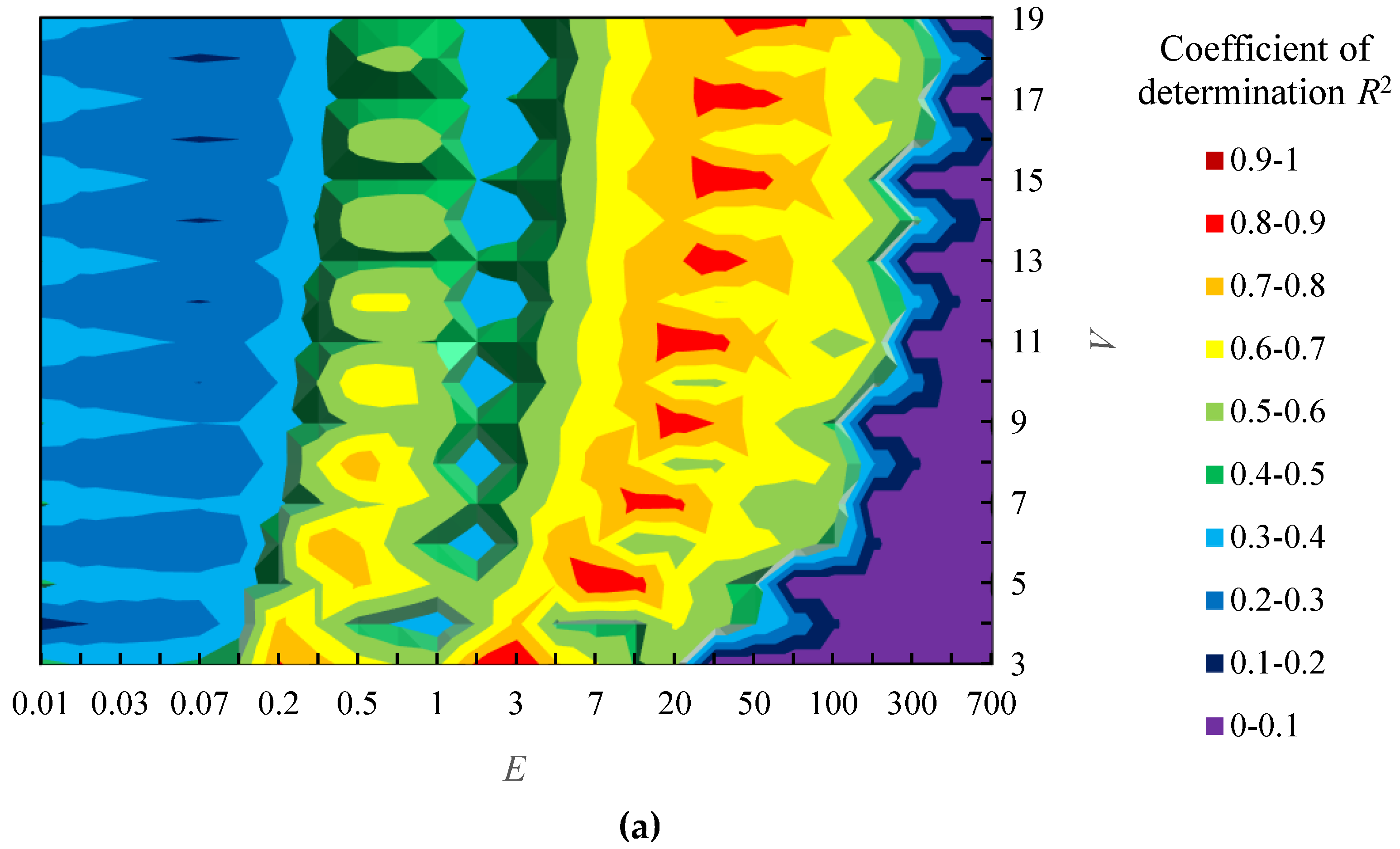
- Combine 2 groups and examine the relationship between parameters (E and V) and coefficient of determination R2 about 10 shapes in the combined groups.
- (iii)
- As same as sample shapes A, divide samples shapes B into 3 groups (Group B1, B2 and B3) and examine the relationship between parameters and R2 in combination of 2 groups.


References
- Ujiie, Y.; Kato, T.; Sato, K.; Matsuoka, Y. Curvature entropy for curved profile generation. Entropy 2012, 14, 533–558. [Google Scholar] [CrossRef]
- Birkhoff, G.D. Aesthetic Measure; Harvard University Press: Cambridge, UK, 1933. [Google Scholar]
- Eysenck, H.J. The empirical determination of an aesthetic formula. Psychol. Rev. 1941, 48, 83–92. [Google Scholar] [CrossRef]
- Berlyne, D.E. Aesthetics and psychobiology; Appleton Century Crofts: New York City, NY, USA, 1971. [Google Scholar]
- Munsinger, H.; Kessen, W. Uncertainty, structure, and preference. Psychol. Monogr. Gen. Appl. 1964, 78, 1–24. [Google Scholar] [CrossRef]
- Hung, W.K.; Chen, L. Effects of novelty and its dimensions on aesthetic preference in product design. Int. J. Des. 2012, 6, 81–90. [Google Scholar]
- Vitz, P.C. Preference for different amounts of visual complexity. Behav. Sci. 1966, 11, 105–114. [Google Scholar] [CrossRef] [PubMed]
- Backes, A.R.; Bruno, O.M. Medical image retrieval based on complexity analysis. Mach. Vis. Appl. 2010, 21, 217–227. [Google Scholar] [CrossRef]
- Wang, D.; Belyaev, A.; Saleem, W.; Seidel, H. Shape Complexity from Image Similarity; Max-Planck-Institut für Informatik: Saarbrücken, Germany, 2008. [Google Scholar]
- Saleem, W.; Belyaev, A.; Wang, D.; Seidel, H. On visual complexity of 3d shapes. Comput. Graph. 2011, 35, 580–585. [Google Scholar] [CrossRef]
- Farin, G.; Rein, G.; Sapidis, N.; Worsey, A.J. Fairing cubic B-spline curves. Comput. Aided Geom. Des. 1987, 4, 91–103. [Google Scholar] [CrossRef]
- Harada, T.; Yoshimoto, F.; Moriyama, M. An aesthetic curve in industrial design. In Proceedings of the 1999 IEEE Symposium on Visual Languages, Tokyo, Japan, 13–16 September 1999. [Google Scholar]
- Harada, T.; Yoshimoto, F. Automatic curve fairing system using visual languages. In Geometric Modeling: Techniques, Applications, Systems and Tools; Sarfraz, M., Ed.; Springer: Berlin/Heidelberg, Germany, 2001; pp. 301–327. [Google Scholar]
- Miura, T. A general equation o aesthetic curves and its self-affinity. Comput. Aided Des. Appl. 2006, 3, 457–464. [Google Scholar] [CrossRef]
- Inoguchi, J.; Kajiwara, K.; Miura, K.T.; Sato, M.; Schiefe, S.K.; Shimizu, Y. Log-aesthetic curves as similarity geometric analogue of Euler’s elasticae. Comput. Aided Geom. Des. 2018, 61, 1–5. [Google Scholar] [CrossRef]
- Ujiie, Y.; Matsuoka, Y. Total absolute curvature to represent the complexity of diverse curved profiles. In Proceedings of the 6th Asian Design Conference, Tsukuba, Ibaraki, Japan, 14–17 October 2003. [Google Scholar]
- Matsumoto, T.; Sato, K.; Matsuoka, Y.; Kato, T. Quantification of “complexity” in curved surface shape using total absolute curvature. Comput. Graph. 2019, 78, 108–115. [Google Scholar] [CrossRef]
- Shannon, C.E. A mathematical theory of communication. Bell Syst. Tech. J. 1948, 27, 379–423, 623–656. [Google Scholar] [CrossRef]
- Owen, J.S. A Survey of Unstructured Mesh Generation Technology. In Proceedings of the 7th International Meshing Roundtable, Livermore, CA, USA, 26–28 October 1998. [Google Scholar]
- Surazhsky, T.; Magid, E.; Soldea, O.; Elber, G.; Rivlin, E. A comparison of Gaussian and mean curvatures estimation methods on triangular meshes. In Proceedings of the 2003 IEEE International Conference on Robotics and Automation, Taipei, Taiwan, 14–19 September 2003. [Google Scholar]
- Endres, D.; Földiák, P. Bayesian Bin Distribution Inference and Mutual Information. IEEE Trans. Inf. Theory 2005, 51, 3766–3779. [Google Scholar] [CrossRef]
- Hughes, T.J.R.; Cottrell, J.A.; Bazilevs, Y. Isogeometric analysis: CAD, finite elements, NURBS, exact geometry and mesh refinement. Comput. Method Appl. Mech. Eng. 2005, 194, 4135–4195. [Google Scholar] [CrossRef]
- Kennedy, J.; Eberhart, R.C. Particle swarm optimization. In Proceedings of the 1995 IEEE Conference of Neural Networks, Perth, Western Australia, Australia, 27 November–1 December 1995. [Google Scholar]


© 2020 by the authors. Licensee MDPI, Basel, Switzerland. This article is an open access article distributed under the terms and conditions of the Creative Commons Attribution (CC BY) license (http://creativecommons.org/licenses/by/4.0/).
Share and Cite
Okano, A.; Matsumoto, T.; Kato, T. Gaussian Curvature Entropy for Curved Surface Shape Generation. Entropy 2020, 22, 353. https://doi.org/10.3390/e22030353
Okano A, Matsumoto T, Kato T. Gaussian Curvature Entropy for Curved Surface Shape Generation. Entropy. 2020; 22(3):353. https://doi.org/10.3390/e22030353
Chicago/Turabian StyleOkano, Akihiro, Taishi Matsumoto, and Takeo Kato. 2020. "Gaussian Curvature Entropy for Curved Surface Shape Generation" Entropy 22, no. 3: 353. https://doi.org/10.3390/e22030353
APA StyleOkano, A., Matsumoto, T., & Kato, T. (2020). Gaussian Curvature Entropy for Curved Surface Shape Generation. Entropy, 22(3), 353. https://doi.org/10.3390/e22030353