A Novel Counterfeit Feature Extraction Technique for Exposing Face-Swap Images Based on Deep Learning and Error Level Analysis


Abstract
1. Introduction
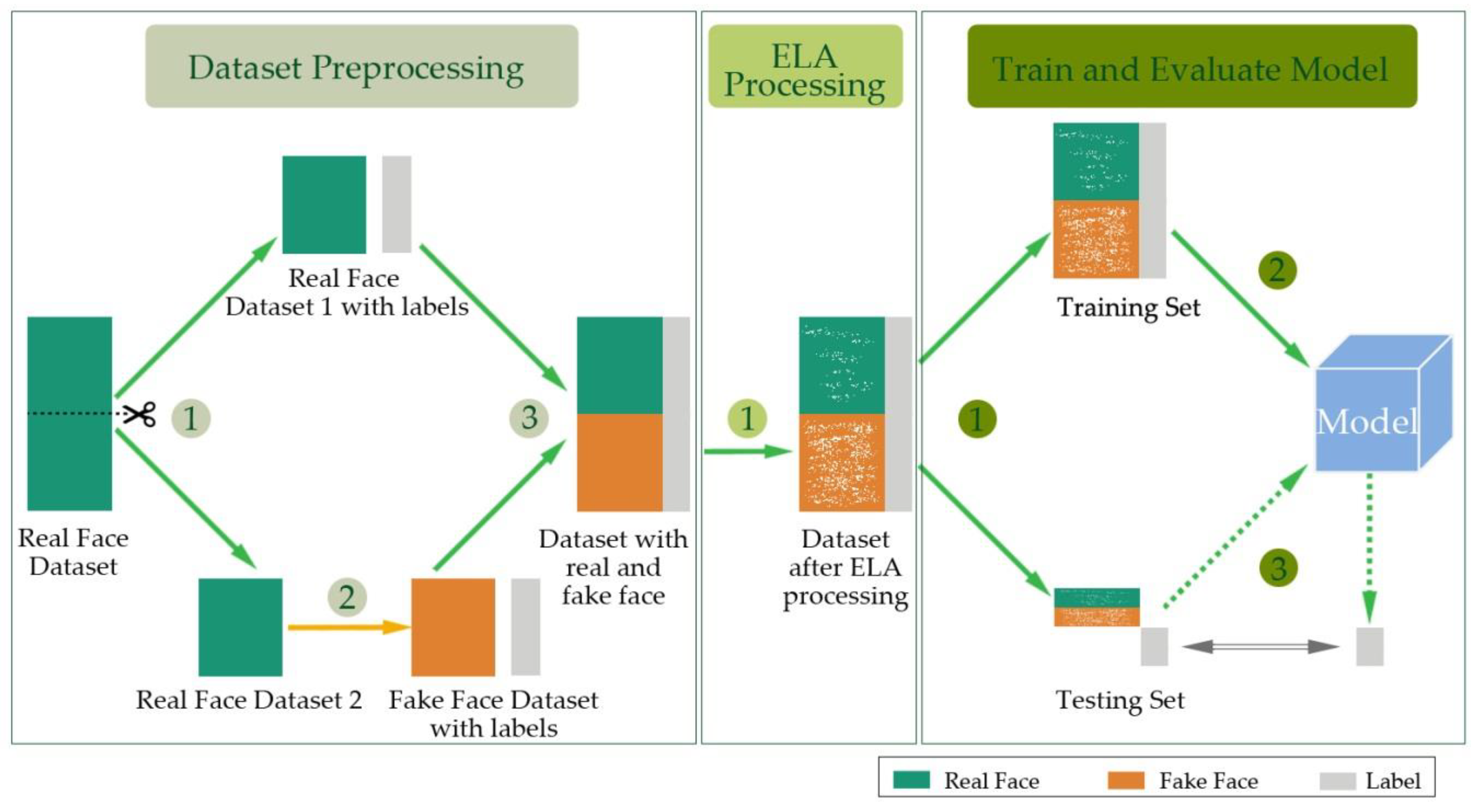
2. Outline of the Proposed Method
3. Methods
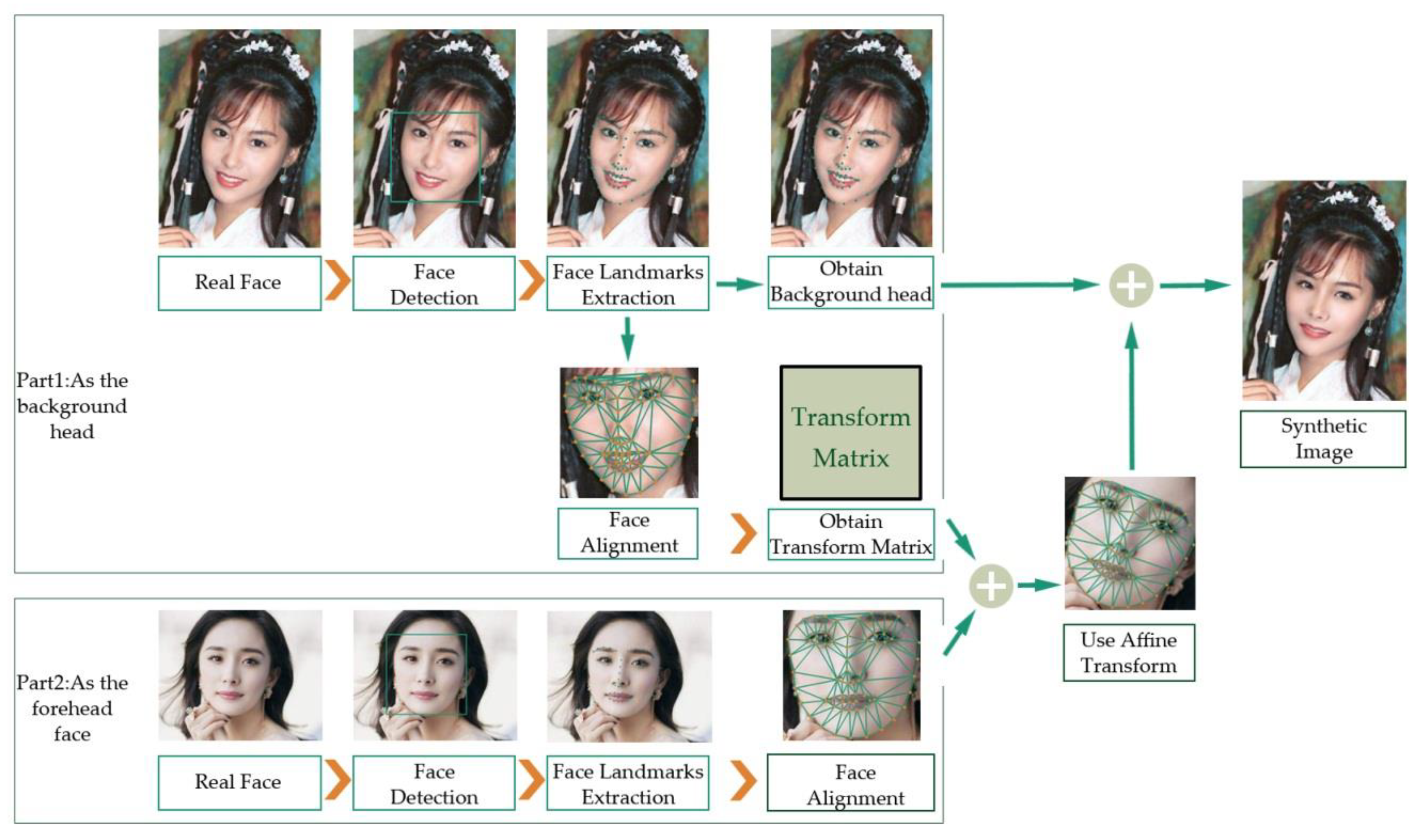
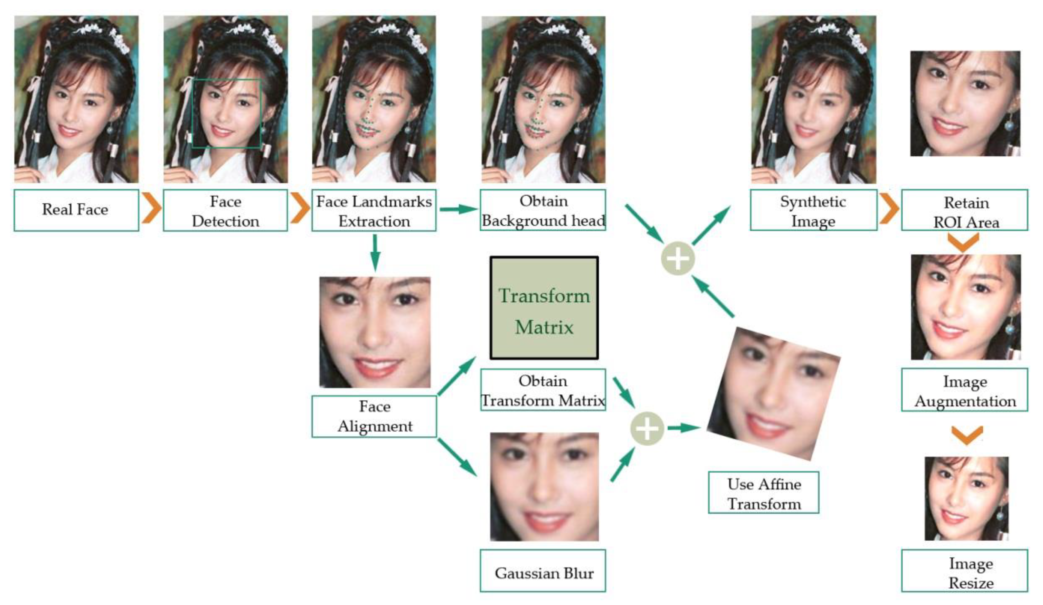
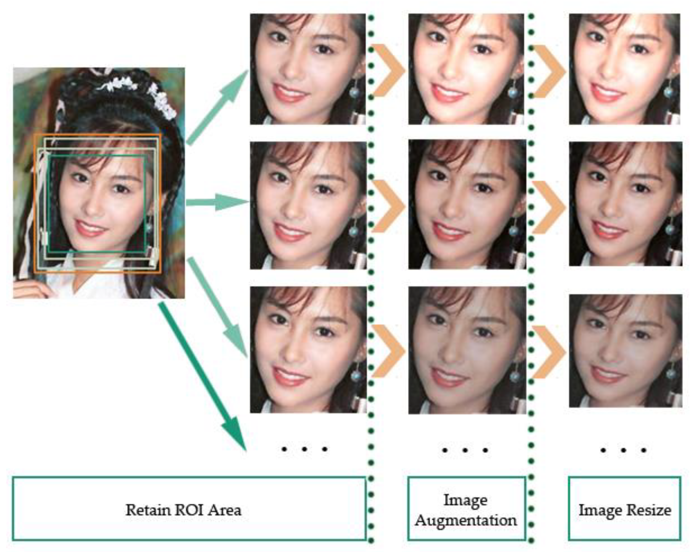
3.1. Dataset Preprocessing
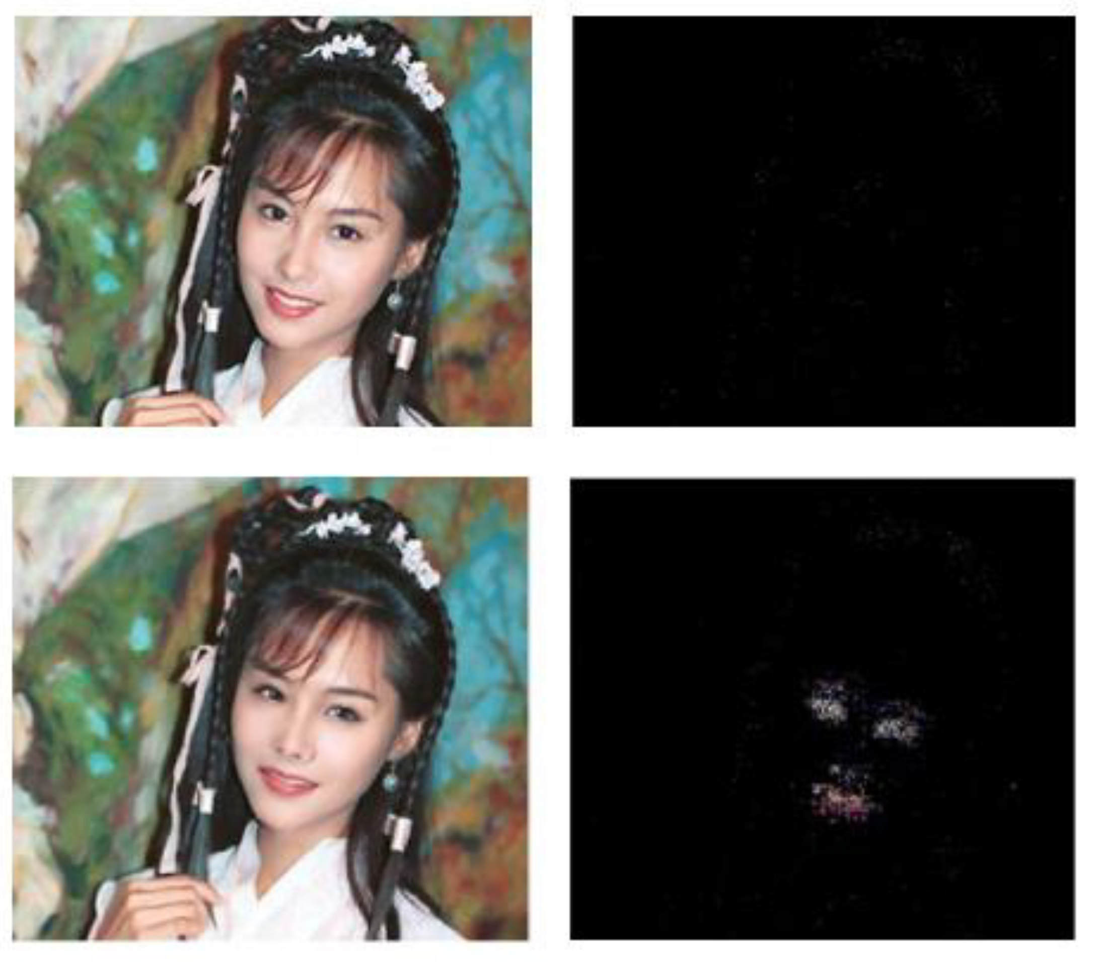
3.2. The Error Level Analysis Processing
- Save the original image and compress the input image to generate a new image according to the specified quality factor.
- Calculate the absolute value of the difference between the two images pixel by pixel, and generate a difference set image.
- According to the biggest pixel value of the difference set, we obtain the enhancement factor.
- Adjust the brightness of the difference set image according to the enhancement factor, and generate the final enhancement ELA image.
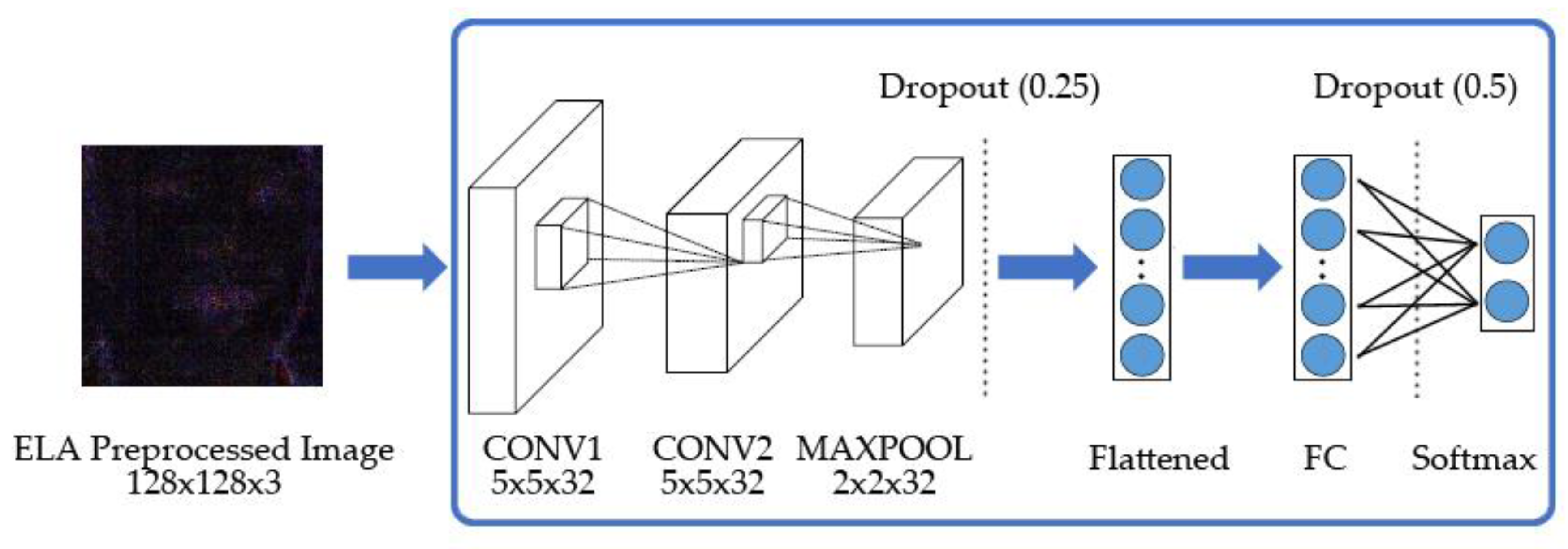
3.3. CNN Architectures
4. Experiments
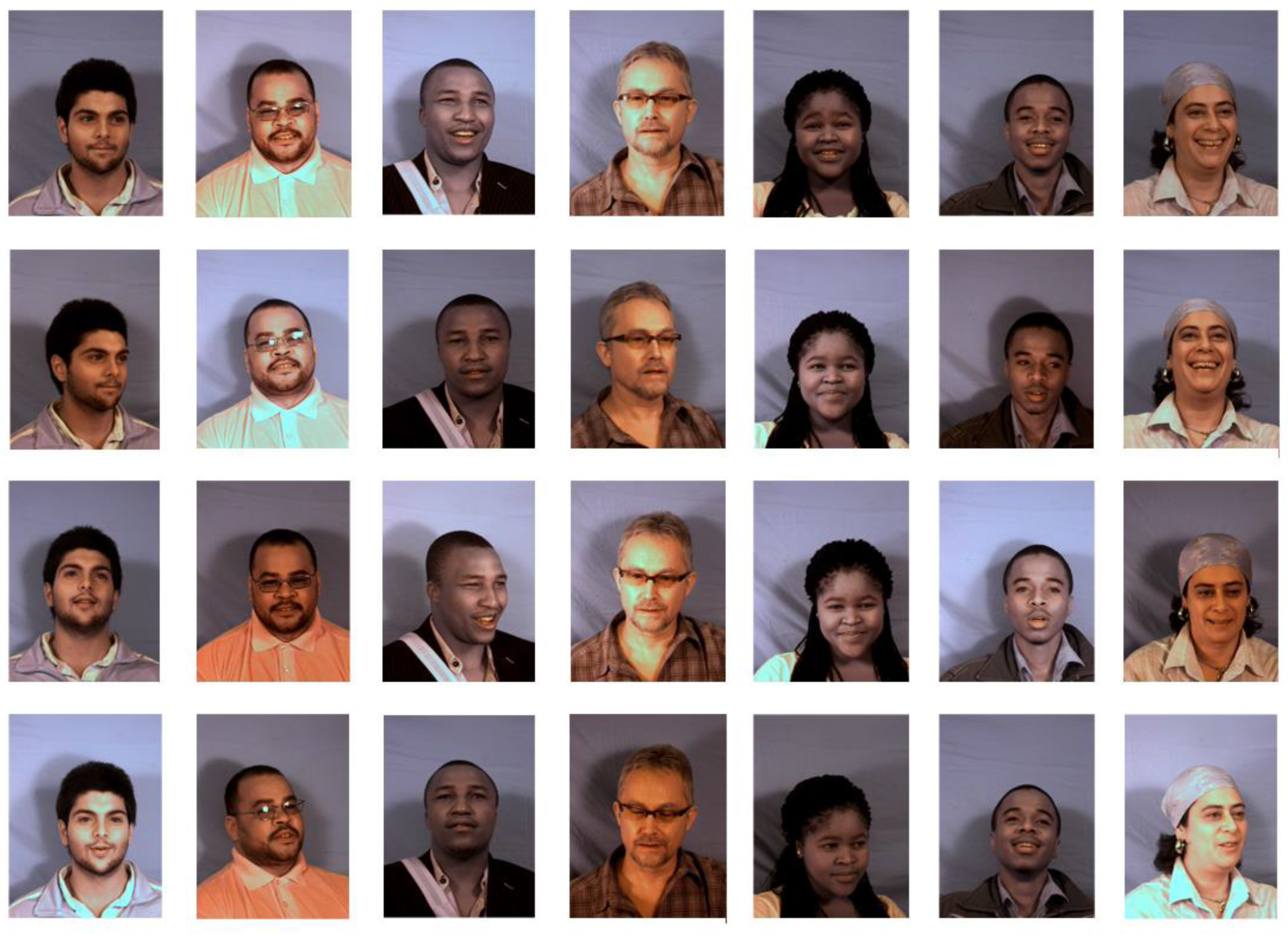
4.1. The Milborrow University of Cape Town Database
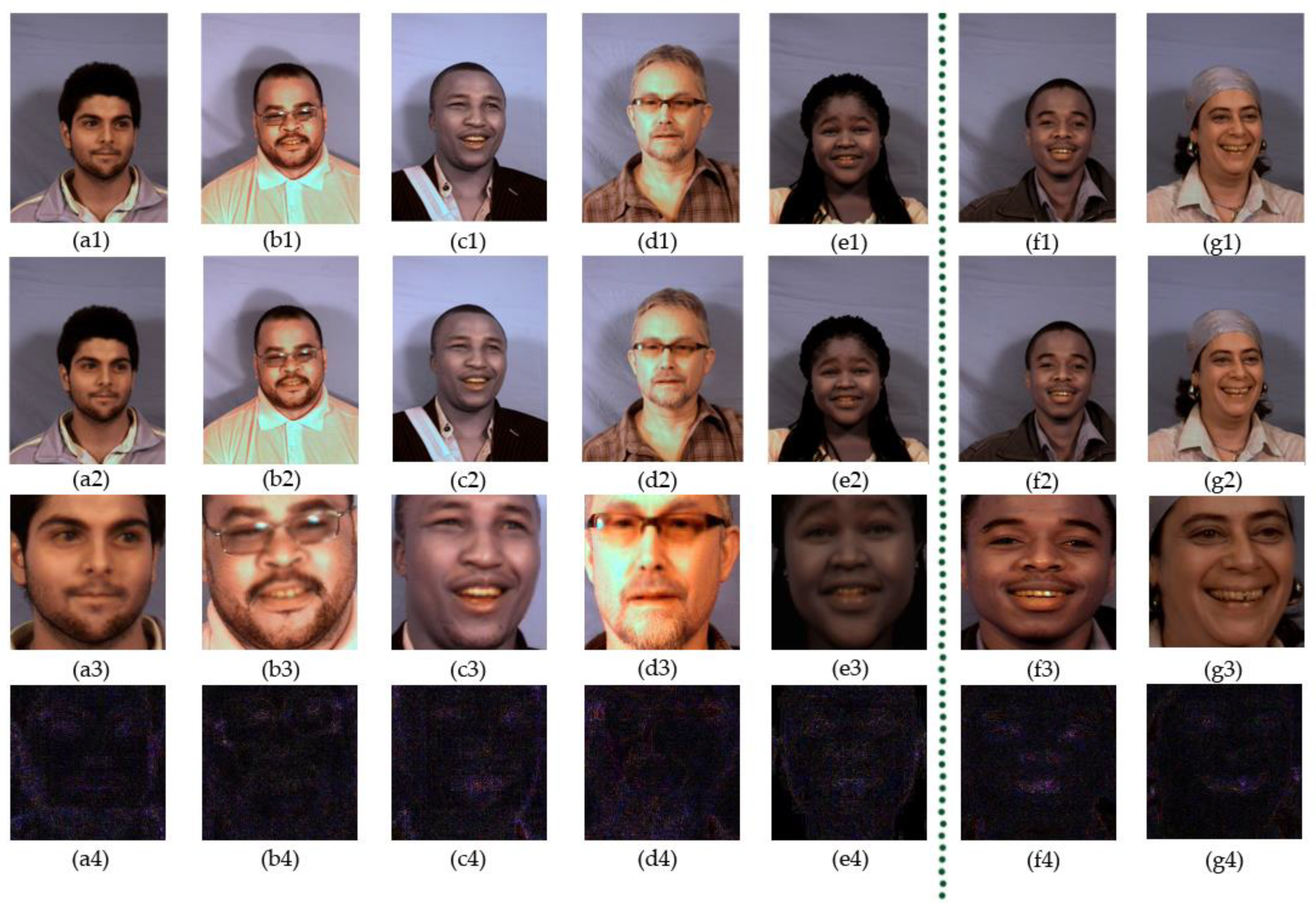
4.2. Dataset Preprocessing and ELA Processing
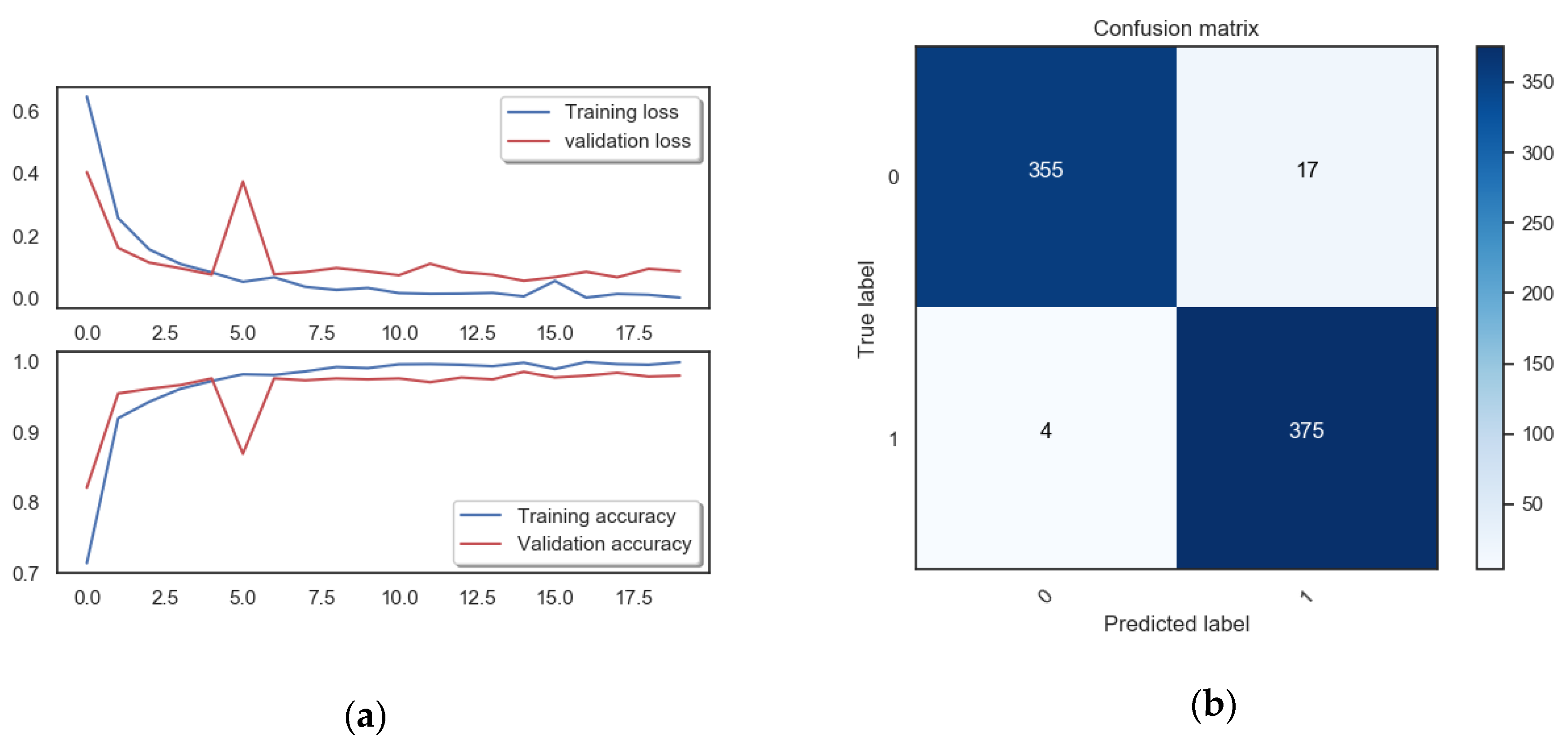
4.3. Train and Evaluate Model
4.4. Comparison with Other Methods
5. Conclusions
Author Contributions
Funding
Conflicts of Interest
References
- Liu, M.Y.; Breuel, T.; Kautz, J. Unsupervised Image-to-Image Translation Networks. In Proceedings of the Advances in Neural Information Processing Systems, Long Beach, CA, USA, 4–9 December 2017; pp. 700–708. [Google Scholar]
- Deep Fake Github. Available online: https://github.com/deepfakes/faceswap (accessed on 29 October 2018).
- Goodfellow, I.; Pouget-Abadie, J.; Mirza, M.; Xu, B.; Warde-Farley, D.; Ozair, S.; Courville, A.; Bengio, Y. Generative adversarial nets. In NIPS’14, Proceedings of the 27th International Conference on Neural Information Processing Systems; MIT Press: Cambridge, MA, USA, 2014; pp. 2672–2680. [Google Scholar]
- Schetinger, V.; Oliveira, M.M.; Da Silva, R.; Carvalho, T.J. Humans are easily fooled by digital images. Comput. Graph. 2017, 68, 142–151. [Google Scholar] [CrossRef]
- Korshunov, P.; Marcel, S. DeepFakes: A New Threat to Face Recognition? Assessment and Detection. arXiv 2018, arXiv:1812.08685. [Google Scholar]
- Li, Y.; Lyu, S. Exposing DeepFake Videos by Detecting Face Warping Artifacts. In Proceedings of the IEEE Conference on Computer Vision and Pattern Recognition Workshops (CVPRW), Long Beach, CA, USA, 16–20 June 2019. [Google Scholar]
- Simonyan, K.; Zisserman, A. Very deep convolutional networks for large-scale image recognition. arXiv 2014, arXiv:1409.1556. [Google Scholar]
- He, K.; Zhang, X.; Ren, S.; Sun, J. Deep residual learning for image recognition. In Proceedings of the CVPR, Las Vegas, NV, USA, 27–30 June 2016. [Google Scholar]
- Afchar, D.; Nozick, V.; Yamagishi, J.; Echizen, I. Mesonet: A compact facial video forgery detection network. In Proceedings of the IEEE International Workshop on Information Forensics and Security (WIFS), Hong Kong, China, 11–13 December 2018. [Google Scholar]
- Thies, J.; Zollhofer, M.; Stamminger, M.; Theobalt, C.; Nießner, M. Face2Face: Real-Time Face Capture and Reenactment of RGB Videos. In Proceedings of the IEEE Conference on Computer Vision and Pattern Recognition, Las Vegas, NV, USA, 27–30 June 2016; pp. 2387–2395. [Google Scholar]
- Li, Y.; Chang, M.C.; Lyu, S. In ictu oculi: Exposing ai generated fake face videos by detecting eye blinking. In Proceedings of the IEEE International Workshop on Information Forensics and Security (WIFS), Hong Kong, China, 11–13 December 2018. [Google Scholar]
- Li, H.; Li, B.; Tan, S.; Huang, J. Detection of deep network generated images using disparities in color components. arXiv 2018, arXiv:1808.07276. [Google Scholar]
- Yang, X.; Li, Y.; Lyu, S. Exposing Deep Fakes Using Inconsistent Head Poses. In Proceedings of the International Conference on Acoustics Speech and Signal Processing, Brighton, UK, 12–17 May 2019; pp. 8261–8265. [Google Scholar]
- Zhou, P.; Han, X.; Morariu, V.I.; Davis, L.S. Two-Stream Neural Networks for Tampered Face Detection. In Proceedings of the 2017 IEEE Conference on Computer Vision and Pattern Recognition Workshops (CVPRW), Honolulu, HI, USA, 21–26 July 2017. [Google Scholar]
- Cpatel, H.; Patel, M.M. An Improvement of Forgery Video Detection Technique using Error Level Analysis. Int. J. Comput. Appl. 2015, 111, 26–28. [Google Scholar] [CrossRef]
- Jeronymo, D.C.; Borges YC, C.; Dos Santos Coelho, L. Image Forgery Detection by Semi-Automatic Wavelet Soft-Thresholding with Error Level Analysis. Expert Syst. Appl. 2017, 85, 348–356. [Google Scholar] [CrossRef]
- Sudiatmika, I.B.K.; Rahman, F.; Trisno, T. Image forgery detection using error level analysis and deep learning. Telkomnika 2019, 17, 653–659. [Google Scholar] [CrossRef]
- Krawetz, N. A picture’s worth digital image analysis and forensics. In Proceedings of the 2007 Black Hat Briefings, Caesars Palace, LV, USA, 31 July–2 August 2007; pp. 1–31. [Google Scholar]
- Zhu, H.; Chen, X.; Dai, W.; Fu, K.; Ye, Q.; Jiao, J. Orientation robust object detection in aerial images using deep convolutional neural network. In Proceedings of the 2015 IEEE International Conference on Image Processing (ICIP), Quebec City, QC, Canada, 27–30 September 2015; pp. 3735–3739. [Google Scholar]
- Garcia, C.; Delakis, M. Convolutional face finder: A neural architecture for fast and robust face detection. IEEE Trans. Pattern Anal. Mach. Intell. 2004, 26, 1408–1423. [Google Scholar] [CrossRef] [PubMed]
- Lawrence, S.; Giles, C.L.; Tsoi, A.C.; Back, A.D. Face recognition: A convolutional neural-network approach. IEEE Trans. Neural Netw. 1997, 8, 98–113. [Google Scholar] [CrossRef] [PubMed]
- Karpathy, A.; Toderici, G.; Shetty, S.; Leung, T.; Sukthankar, R.; Fei-Fei, L. Large-Scale Video Classification with Convolutional Neural Networks. In Proceedings of the 2014 IEEE Conference on Computer Vision and Pattern Recognition, Columbus, OH, USA, 23–28 June 2014; pp. 1725–1732. [Google Scholar]
- Dong, C.; Loy, C.C.; He, K.; Tang, X. Image Super-Resolution Using Deep Convolutional Networks. IEEE Trans. Pattern Anal. Mach. Intell. 2016, 38, 295–307. [Google Scholar] [CrossRef] [PubMed]
- Ng, T.T.; Hsu, J.; Chang, S.F. Columbia Image Splicing Detection Evaluation Dataset. Available online: http://www.ee.columbia.edu/ln/dvmm/downloads/AuthSplicedDataSet/AuthSplicedDataSet.htm (accessed on 30 March 2008).
- Dong, J.; Wang, W.; Tan, T. Casia Image Tampering Detection Evaluation Database 2010. Available online: http://forensics.idealtest.org (accessed on 21 February 2020).
- Dong, J.; Wang, W.; Tan, T. Casia image tampering detection evaluation database. In Signal and Information Processing (ChinaSIP), Proceedings of the 2013 IEEE China Summit & International Conference, Beijing, China, 6–10 July 2013; IEEE: Piscataway, NJ, USA, 2013; pp. 422–426. [Google Scholar]
- De Carvalho, T.J.; Riess, C.; Angelopoulou, E.; Pedrini, H.; de Rezende Rocha, A. Exposing digital image forgeries by illumination color classification. IEEE Trans. Inf. Forensics Secur. 2013, 8, 1182–1194. [Google Scholar] [CrossRef]
- MUCT Database. Available online: https://github.com/StephenMilborrow/muct (accessed on 21 February 2020).
- CVPRW2019_Face_Artifacts. Available online: https://github.com/danmohaha/CVPRW2019_Face_Artifacts (accessed on 16 June 2019).
- Koshy, R.; Mahmood, A. Optimizing Deep CNN Architectures for Face Liveness Detection. Entropy 2019, 21, 423. [Google Scholar] [CrossRef]
- Schetinger, V.; Iuliani, M.; Piva, A.; Oliveira, M.M. Image forgery detection confronts image composition. Comput. Graph. 2017, 68, 152–163. [Google Scholar] [CrossRef]


| Level Class | Combination with Forensics | Typical Examples |
|---|---|---|
| Level 1 | —— | four CNN models [6] |
| Level 2 | —— | MesoNet [9] |
| Level 3 | abnormal physiological signal | breathing, pulse, eye blinking [11], head positions [13] |
| Consistency of imaging equipment | Local noise residuals and camera characteristics [14] | |
| abnormal computer generated image | color difference [12] |
| Model | Space Complexity | Time Complexity | Practical Experiment | |||
|---|---|---|---|---|---|---|
| Weight Layers | Model Size (Parameters) | Model Size (MB) | GFLOPs (Forward Pass) | Training Epoch | Testing AUC | |
| VGG16 | 16 | 1.38 108 | 528 MB | 15.5 | 100 | 83.3% |
| ResNet50 | 50 | 2.56 107 | 98 MB | 3.9 | 20 | 95.4% |
| ResNet101 | 101 | 4.46 107 | 542 MB | 7.6 | 20 | 95.1% |
| ResNet152 | 152 | 6.03 107 | 736 MB | 11.3 | 20 | 93.8% |
| Our method | 3 | 2.95 107 | 225 MB | 0.44 | 9 | 97.6% |
© 2020 by the authors. Licensee MDPI, Basel, Switzerland. This article is an open access article distributed under the terms and conditions of the Creative Commons Attribution (CC BY) license (http://creativecommons.org/licenses/by/4.0/).
Share and Cite
Zhang, W.; Zhao, C.; Li, Y. A Novel Counterfeit Feature Extraction Technique for Exposing Face-Swap Images Based on Deep Learning and Error Level Analysis. Entropy 2020, 22, 249. https://doi.org/10.3390/e22020249
Zhang W, Zhao C, Li Y. A Novel Counterfeit Feature Extraction Technique for Exposing Face-Swap Images Based on Deep Learning and Error Level Analysis. Entropy. 2020; 22(2):249. https://doi.org/10.3390/e22020249
Chicago/Turabian StyleZhang, Weiguo, Chenggang Zhao, and Yuxing Li. 2020. "A Novel Counterfeit Feature Extraction Technique for Exposing Face-Swap Images Based on Deep Learning and Error Level Analysis" Entropy 22, no. 2: 249. https://doi.org/10.3390/e22020249
APA StyleZhang, W., Zhao, C., & Li, Y. (2020). A Novel Counterfeit Feature Extraction Technique for Exposing Face-Swap Images Based on Deep Learning and Error Level Analysis. Entropy, 22(2), 249. https://doi.org/10.3390/e22020249