Nonlinear Canonical Correlation Analysis:A Compressed Representation Approach


Abstract
1. Introduction
2. Previous Work
3. Problem Formulation
4. Iterative Projections Solution
Optimality Conditions
- 1.
- 2.
| Algorithm 1 Arimoto Blahut pseudocode for rate distortion with second order statistics constraints |
| Require: Ensure: Fix
|
5. Compressed Representation CCA for Empirical Data
5.1. Previous Results
5.2. Our Suggested Method
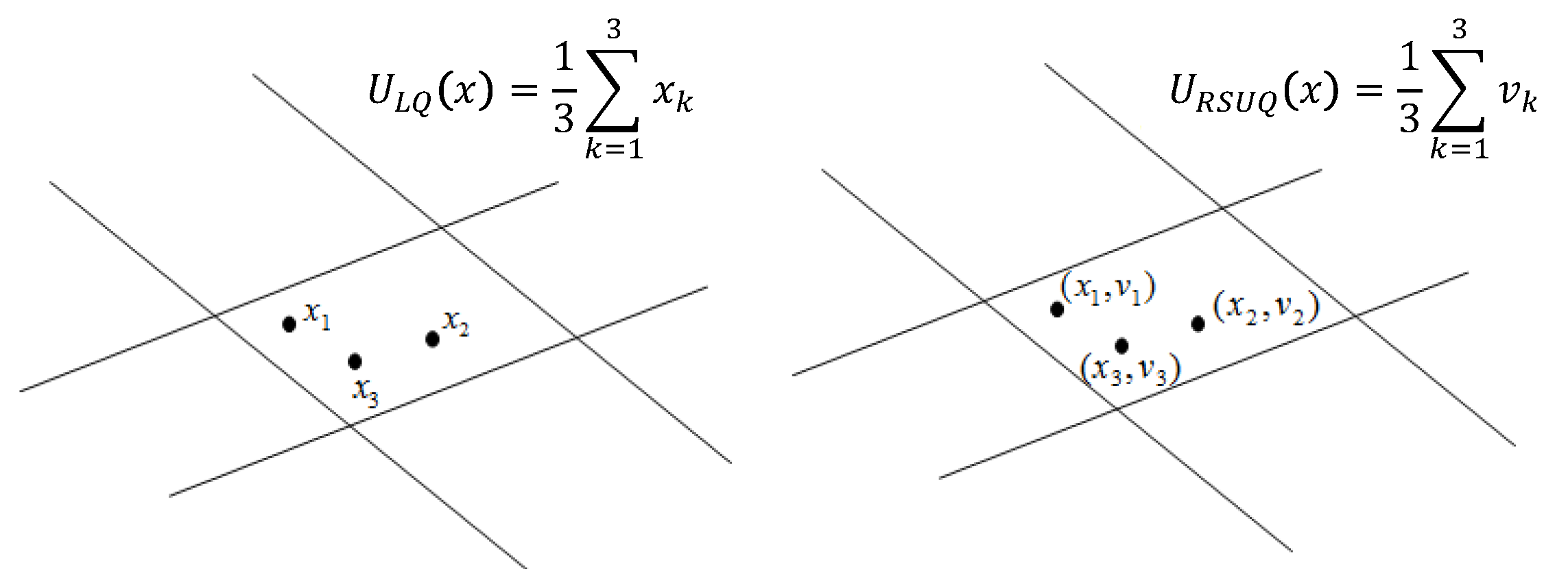
5.2.1. Lattice Quantization
5.2.2. CRCCA by Quantization
| Algorithm 2 A single step of CRCCA by quantization |
Require: , a fixed uniform quantizer
|
5.2.3. Convergence Analysis
5.3. Regularization
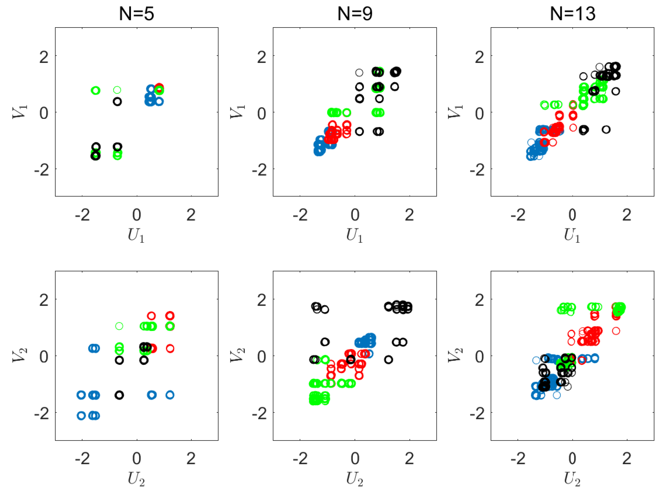
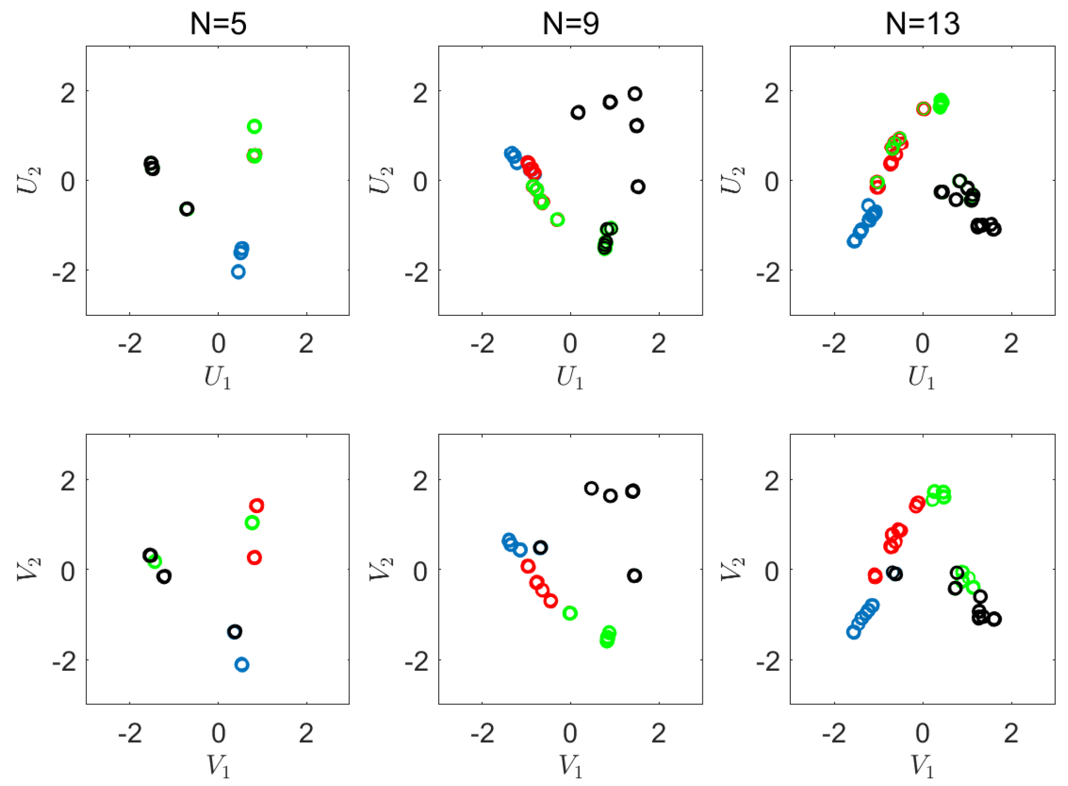
6. Experiments
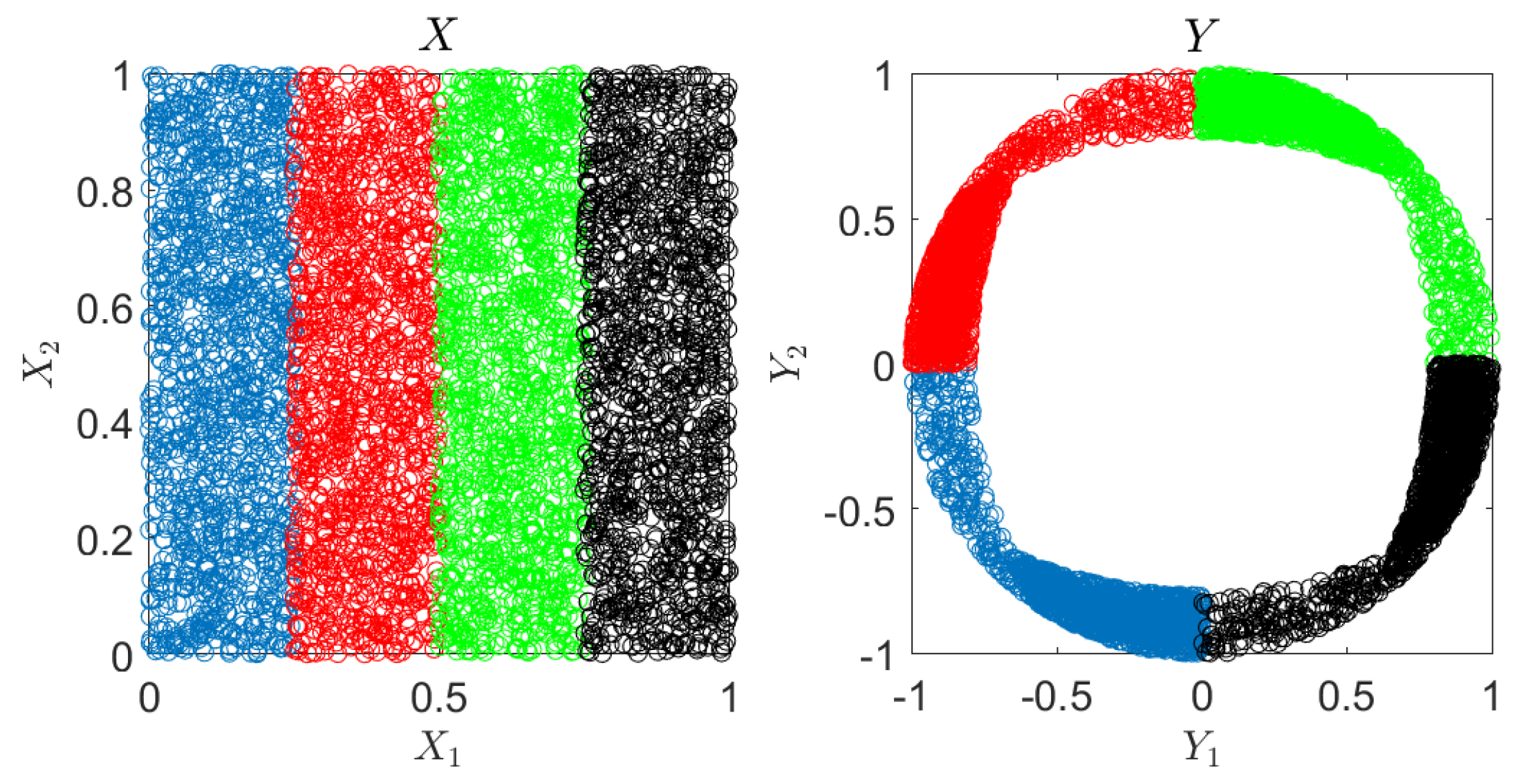
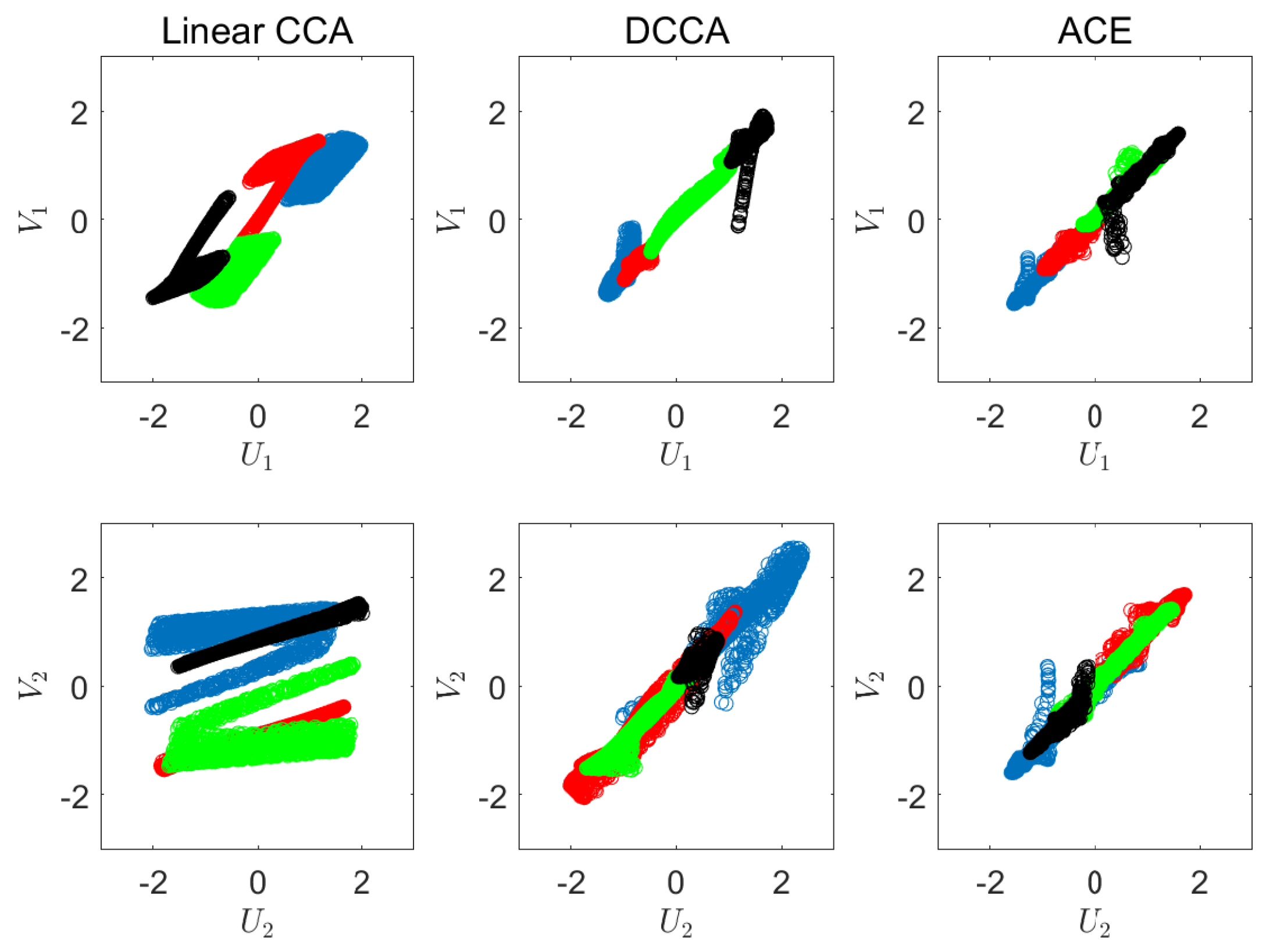
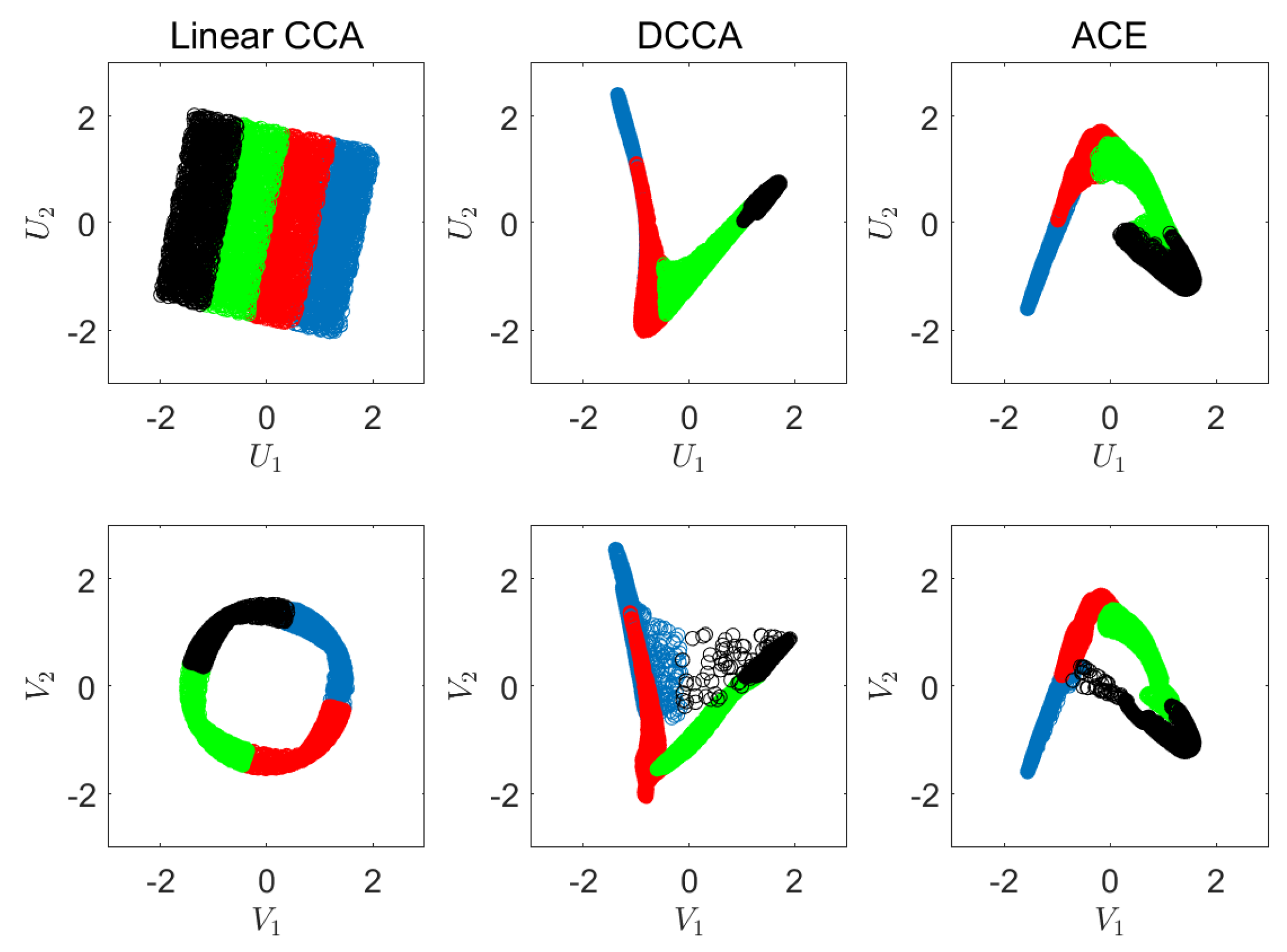
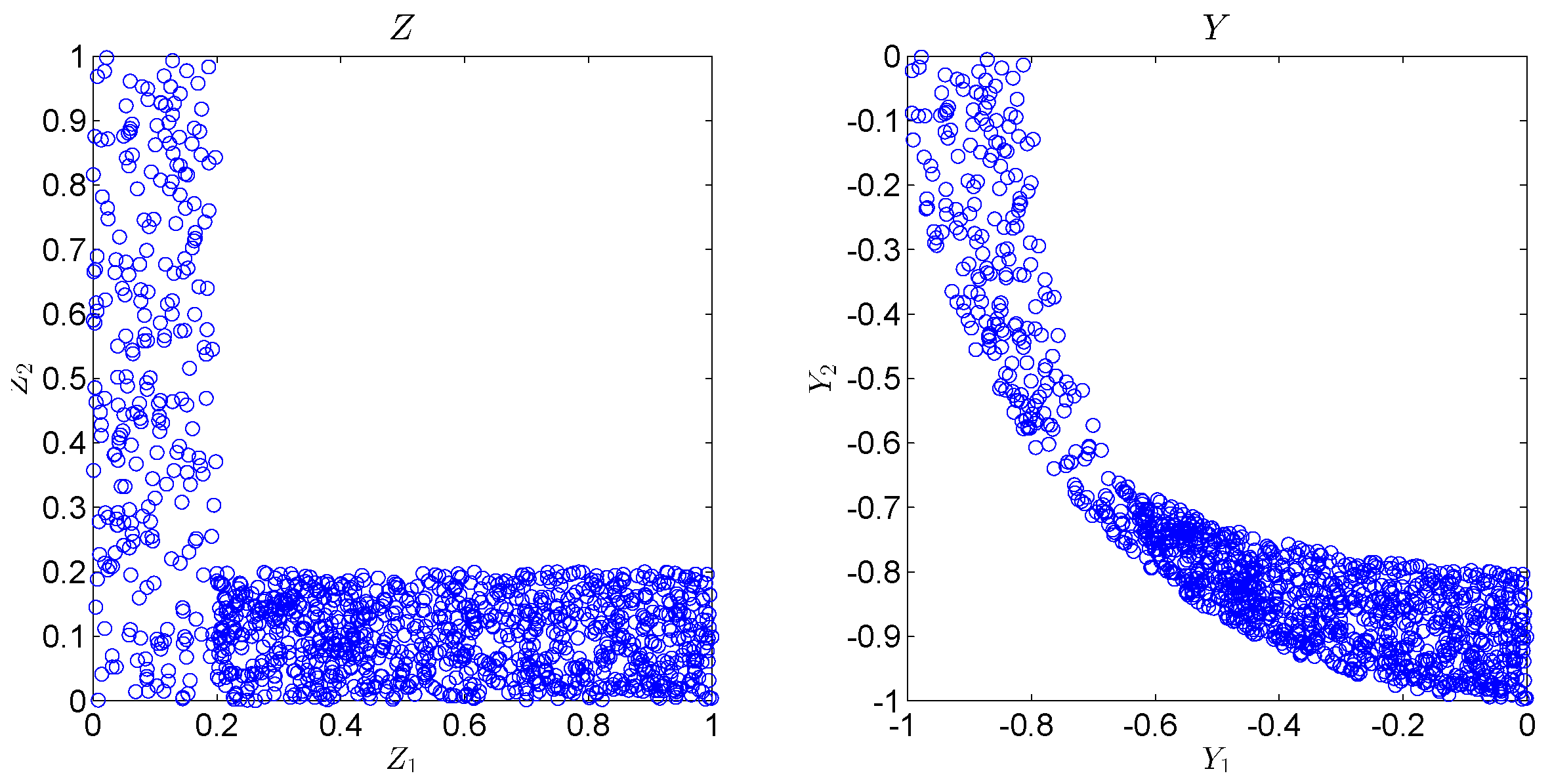
6.1. Synthetic Experiments
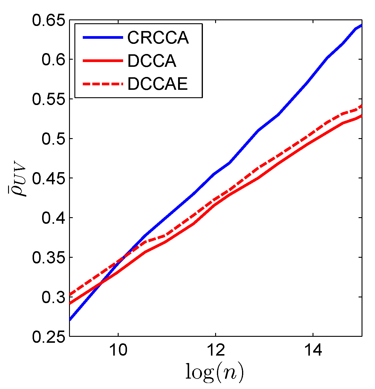
6.2. Real-World Experiment
7. Discussion and Conclusions
Author Contributions
Funding
Conflicts of Interest
Appendix A. A Proof for Lemma 1
Appendix B. A Proof for Lemma 2
Appendix C. Synthetic Experiment Description

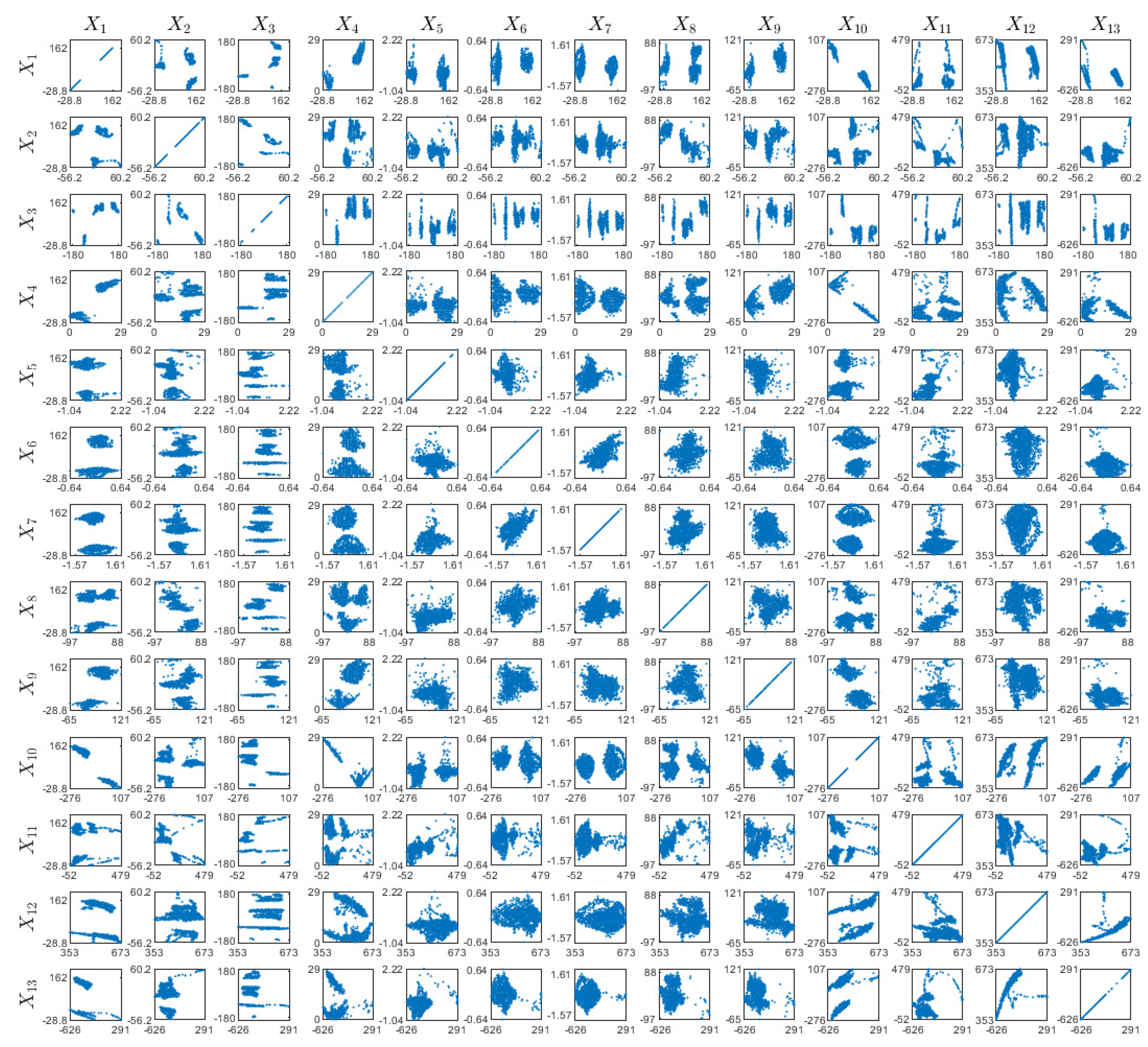
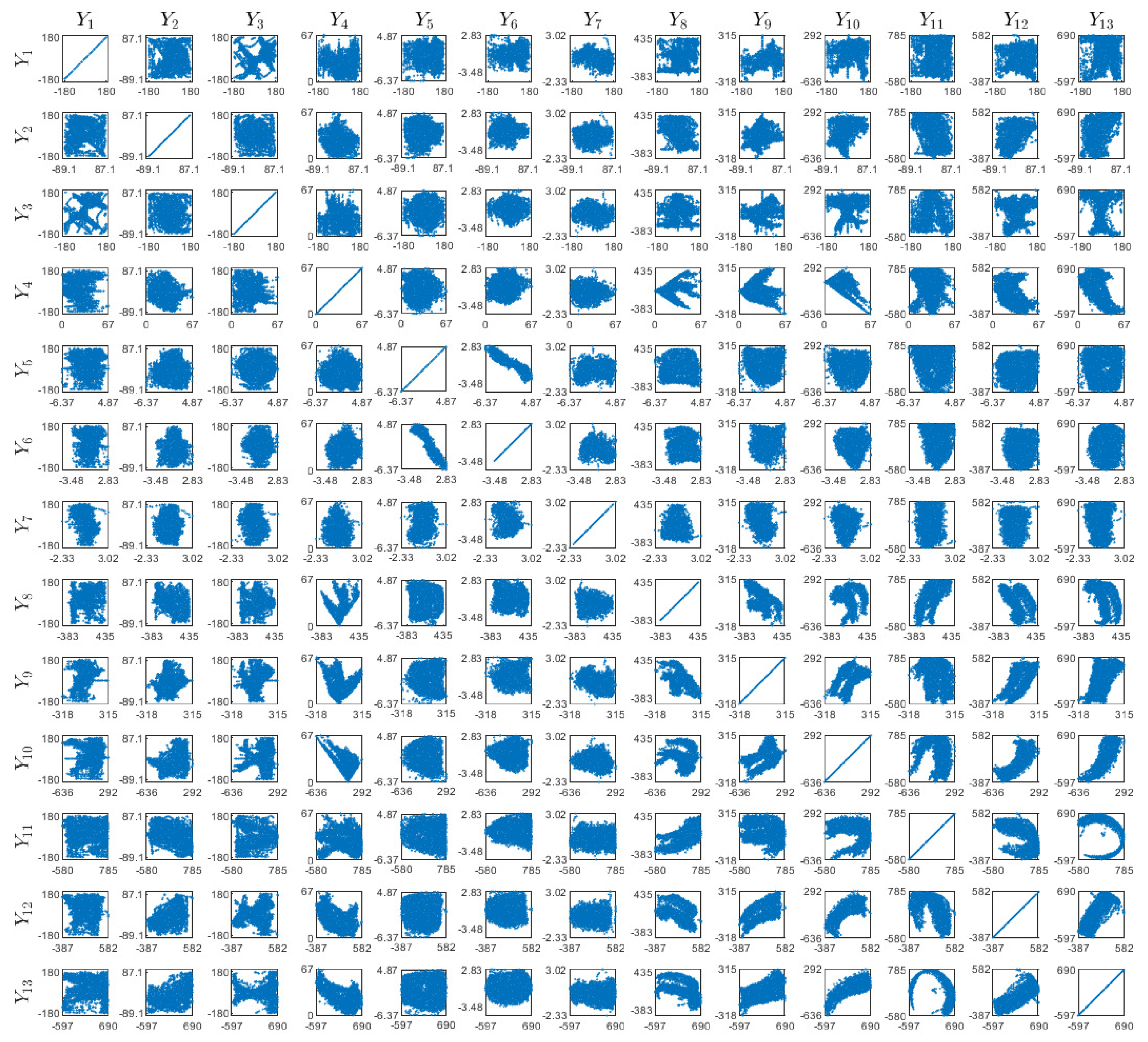
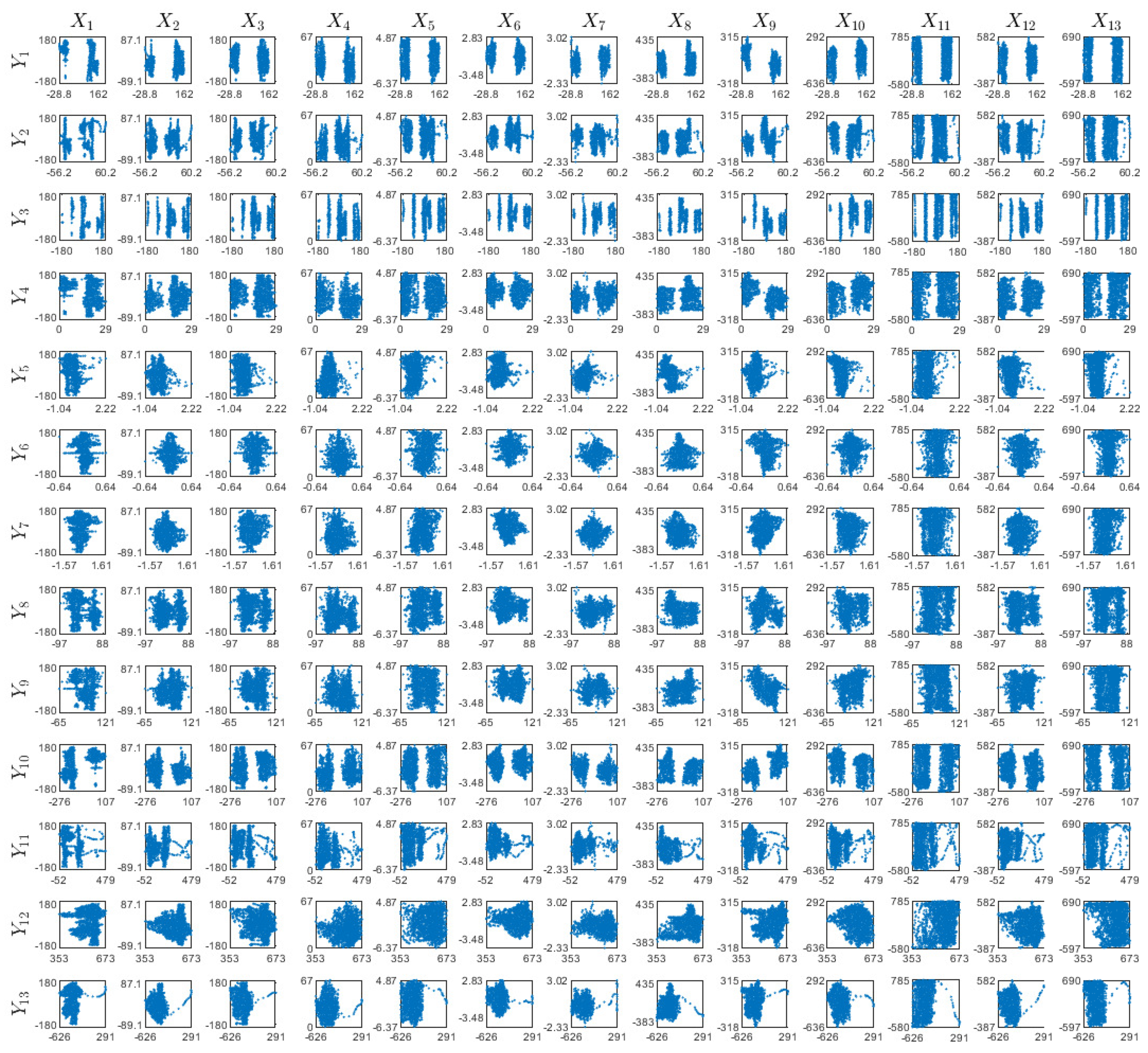
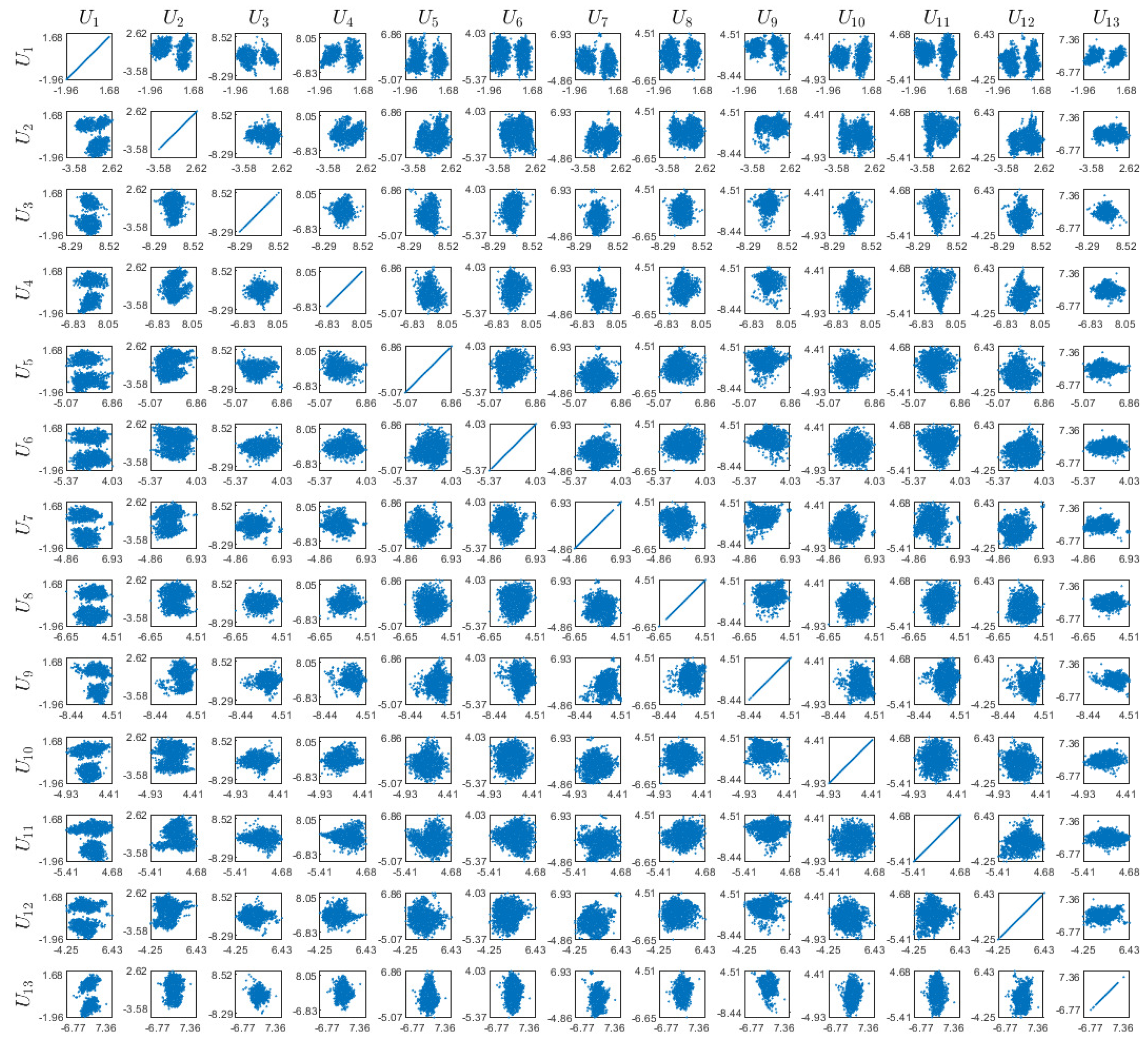
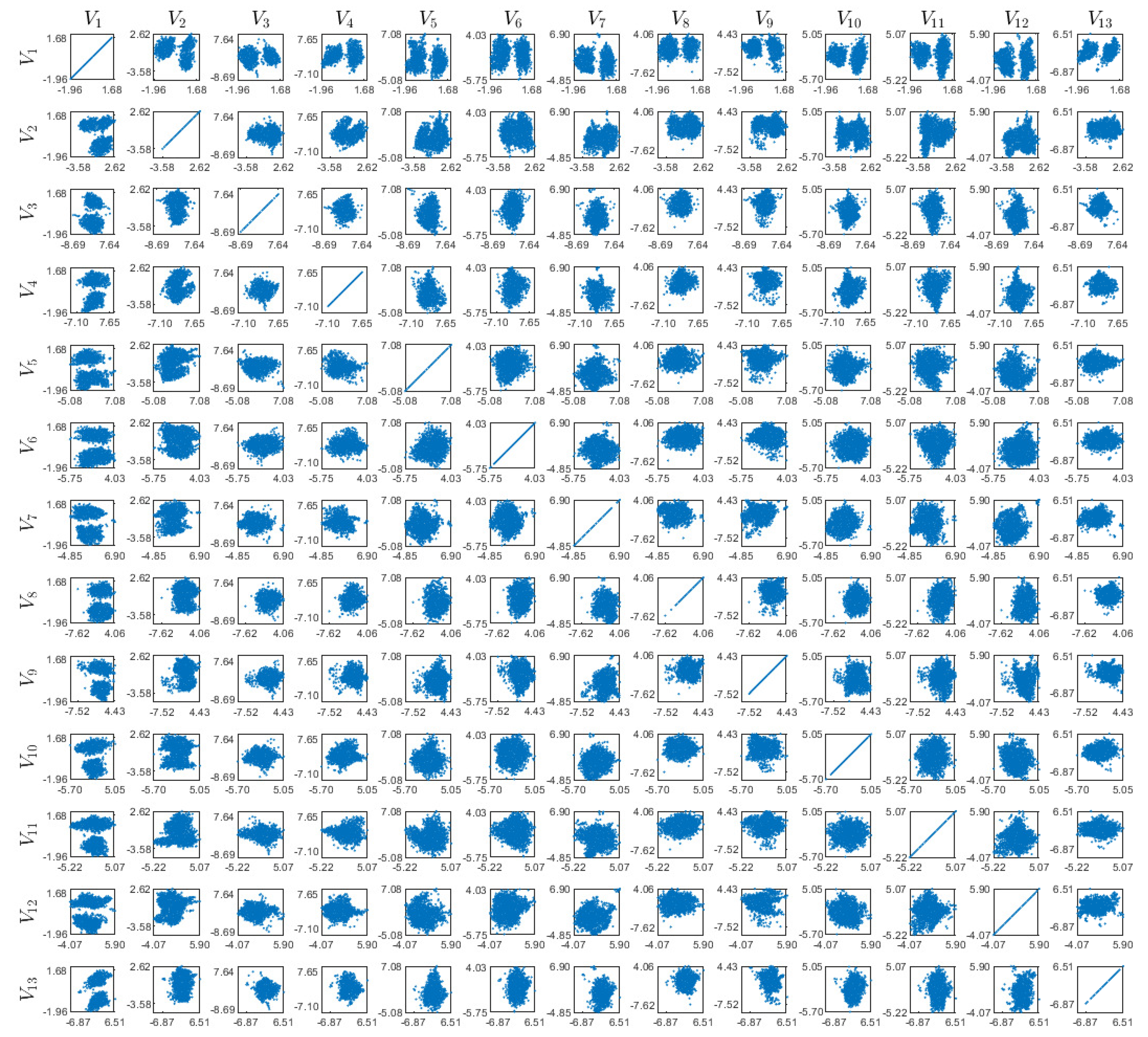
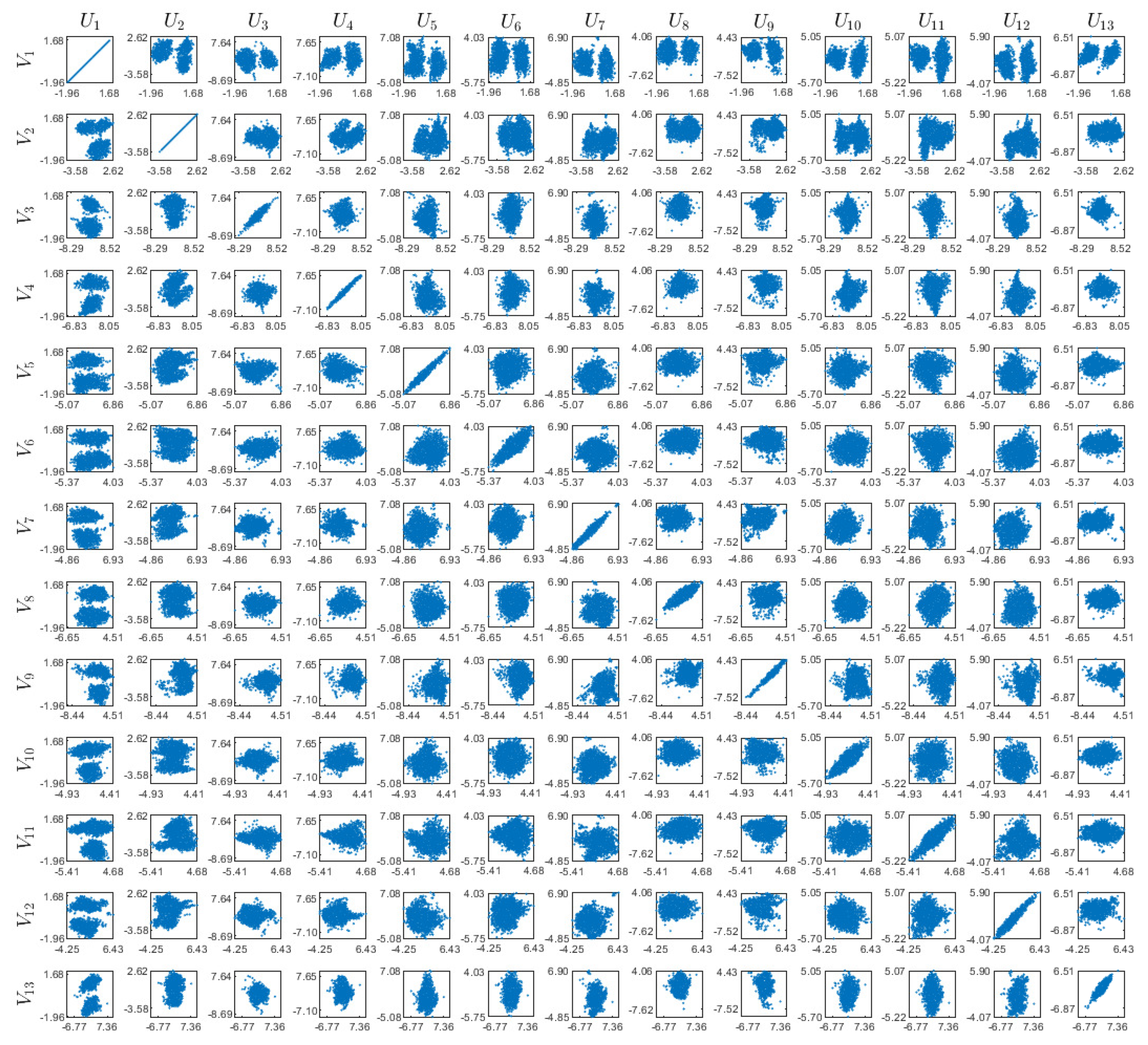
Appendix D. Visualizations of the Real World Experiment


References
- Hotelling, H. Relations between two sets of variates. Biometrika 1936, 28, 321–377. [Google Scholar] [CrossRef]
- Arora, R.; Livescu, K. Kernel CCA for multi-view learning of acoustic features using articulatory measurements. In Proceedings of the Symposium on Machine Learning in Speech and Language Processing, Portland, OR, USA, 14 September 2012; pp. 34–37. [Google Scholar]
- Dhillon, P.; Foster, D.P.; Ungar, L.H. Multi-view learning of word embeddings via cca. In Advances in Neural Information Processing Systems; MIT Press: Cambridge, MA, USA, 2011; pp. 199–207. [Google Scholar]
- Gong, Y.; Wang, L.; Hodosh, M.; Hockenmaier, J.; Lazebnik, S. Improving image-sentence embeddings using large weakly annotated photo collections. In European Conference on Computer Vision; Springer: Berlin/Heidelberg, Germany, 2014; pp. 529–545. [Google Scholar]
- Slaney, M.; Covell, M. Facesync: A linear operator for measuring synchronization of video facial images and audio tracks. In Advances in Neural Information Processing Systems; MIT Press: Cambridge, MA, USA, 2011; pp. 814–820. [Google Scholar]
- Kim, T.K.; Wong, S.F.; Cipolla, R. Tensor canonical correlation analysis for action classification. In Computer Vision and Pattern Recognition; IEEE: Piscataway, NJ, USA, 2007; pp. 1–8. [Google Scholar]
- Van Der Burg, E.; de Leeuw, J. Nonlinear canonical correlation. Br. J. Math. Stat. Psychol. 1983, 36, 54–80. [Google Scholar] [CrossRef]
- Breiman, L.; Friedman, J.H. Estimating optimal transformations for multiple regression and correlation. J. Am. Stat. Assoc. 1985, 80, 580–598. [Google Scholar] [CrossRef]
- Akaho, S. A Kernel Method For Canonical Correlation Analysis. In Proceedings of the International Meeting of the Psychometric Society, Osaka, Japan, 15–19 July 2001. [Google Scholar]
- Wang, C. Variational Bayesian approach to canonical correlation analysis. IEEE Trans. Neural Netw. 2007, 18, 905–910. [Google Scholar] [CrossRef] [PubMed]
- Klami, A.; Virtanen, S.; Kaski, S. Bayesian canonical correlation analysis. J. Mach. Learn. Res. 2013, 14, 965–1003. [Google Scholar]
- Andrew, G.; Arora, R.; Bilmes, J.A.; Livescu, K. Deep canonical correlation analysis. In Proceedings of the 30th International Conference on Machine Learning, Atlanta, GA, USA, 16–21 June 2013; pp. 1247–1255. [Google Scholar]
- Michaeli, T.; Wang, W.; Livescu, K. Nonparametric canonical correlation analysis. In Proceedings of the 33rd International Conference on Machine Learning, New York, NY, USA, 19–24 June 2016; pp. 1967–1976. [Google Scholar]
- Hardoon, D.R.; Szedmak, S.; Shawe-Taylor, J. Canonical correlation analysis: An overview with application to learning methods. Neural Comput. 2004, 16, 2639–2664. [Google Scholar] [CrossRef]
- Wang, W.; Arora, R.; Livescu, K.; Bilmes, J.A. On Deep Multi-View Representation Learning. In Proceedings of the 33rd International Conference on Machine Learning, Lille, France, 6–11 July 2015; pp. 1083–1092. [Google Scholar]
- Arora, R.; Mianjy, P.; Marinov, T. Stochastic optimization for multiview representation learning using partial least squares. In Proceedings of the 33rd International Conference on Machine Learning, New York, NY, USA, 19–24 June 2016; pp. 1786–1794. [Google Scholar]
- Arora, R.; Marinov, T.V.; Mianjy, P.; Srebro, N. Stochastic Approximation for Canonical Correlation Analysis. In Proceedings of the Advances in Neural Information Processing Systems, Long Beach, NY, USA, 4–9 December 2017; pp. 4778–4787. [Google Scholar]
- Wang, W.; Arora, R.; Livescu, K.; Srebro, N. Stochastic optimization for deep CCA via nonlinear orthogonal iterations. In Proceedings of the 53rd Annual Allerton Conference on Communication, Control, and Computing (Allerton), Monticello, IL, USA, 30 September–2 October 2015; IEEE: Piscataway, NJ, USA, 2015; pp. 688–695. [Google Scholar]
- Cover, T.M.; Thomas, J.A. Elements of Information Theory; John Wiley & Sons: Chichester, UK, 2012. [Google Scholar]
- Tishby, N.; Pereira, F.C.; Bialek, W. The information bottleneck method. In Proceedings of the 37th Annual Allerton Conference on Communication, Control and Computing, Monticello, IL, USA, 22–24 December 1999; pp. 368–377. [Google Scholar]
- Ter Braak, C.J. Interpreting canonical correlation analysis through biplots of structure correlations and weights. Psychometrika 1990, 55, 519–531. [Google Scholar] [CrossRef]
- Graffelman, J. Enriched biplots for canonical correlation analysis. J. Appl. Stat. 2005, 32, 173–188. [Google Scholar] [CrossRef]
- Witten, D.M.; Tibshirani, R.; Hastie, T. A penalized matrix decomposition, with applications to sparse principal components and canonical correlation analysis. Biostatistics 2009, 10, 515–534. [Google Scholar] [CrossRef]
- Witten, D.M.; Tibshirani, R.J. Extensions of sparse canonical correlation analysis with applications to genomic data. Stat. Appl. Genet. Mol. Biol. 2009, 8, 1–27. [Google Scholar] [CrossRef]
- Graffelman, J.; Pawlowsky-Glahn, V.; Egozcue, J.J.; Buccianti, A. Exploration of geochemical data with compositional canonical biplots. J. Geochem. Explor. 2018, 194, 120–133. [Google Scholar] [CrossRef]
- Lancaster, H. The structure of bivariate distributions. Ann. Math. Stat. 1958, 29, 719–736. [Google Scholar] [CrossRef]
- Hannan, E. The general theory of canonical correlation and its relation to functional analysis. J. Aust. Math. Soc. 1961, 2, 229–242. [Google Scholar] [CrossRef][Green Version]
- Van der Burg, E.; de Leeuw, J.; Dijksterhuis, G. OVERALS: Nonlinear canonical correlation with k sets of variables. Comput. Stat. Data Anal. 1994, 18, 141–163. [Google Scholar] [CrossRef]
- Gifi, A. Nonlinear Multivariate Analysis; Wiley-VCH: Hoboken, NJ, USA, 1990. [Google Scholar]
- Makur, A.; Kozynski, F.; Huang, S.L.; Zheng, L. An efficient algorithm for information decomposition and extraction. In Proceedings of the 2015 53rd Annual Allerton Conference on Communication, Control, and Computing (Allerton), Monticello, IL, USA, 30 September–2 October 2015; IEEE: Piscataway, NJ, USA, 2015; pp. 972–979. [Google Scholar]
- Lai, P.L.; Fyfe, C. Kernel and nonlinear canonical correlation analysis. Int. J. Neural Syst. 2000, 10, 365–377. [Google Scholar] [CrossRef] [PubMed]
- Uurtio, V.; Bhadra, S.; Rousu, J. Large-Scale Sparse Kernel Canonical Correlation Analysis. In Proceedings of the 36th International Conference on Machine Learning, Long Beach, CA, USA, 10–15 June 2019; pp. 6383–6391. [Google Scholar]
- Yu, J.; Wang, K.; Ye, L.; Song, Z. Accelerated Kernel Canonical Correlation Analysis with Fault Relevance for Nonlinear Process Fault Isolation. Ind. Eng. Chem. Res. 2019, 58, 18280–18291. [Google Scholar] [CrossRef]
- Schölkopf, B.; Herbrich, R.; Smola, A.J. A generalized representer theorem. In International Conference on Computational Learning Theory; Springer: Berlin/Heidelberg, Germany, 2001; pp. 416–426. [Google Scholar]
- Bach, F.R.; Jordan, M.I. Kernel independent component analysis. J. Mach. Learn. Res. 2002, 3, 1–48. [Google Scholar]
- Halko, N.; Martinsson, P.G.; Tropp, J.A. Finding structure with randomness: Probabilistic algorithms for constructing approximate matrix decompositions. SIAM Rev. 2011, 53, 217–288. [Google Scholar] [CrossRef]
- Rissanen, J. Modeling by shortest data description. Automatica 1978, 14, 465–471. [Google Scholar] [CrossRef]
- Chigirev, D.V.; Bialek, W. Optimal Manifold Representation of Data: An Information Theoretic Approach. In Proceedings of the Advances in Neural Information Processing Systems, Vancouver, BC, Canada, 8–13 December 2003; pp. 161–168. [Google Scholar]
- Vera, M.; Piantanida, P.; Vega, L.R. The Role of the Information Bottleneck in Representation Learning. In Proceedings of the 2018 IEEE International Symposium on Information Theory (ISIT), Vail, CO, USA, 17–22 June 2018; IEEE: Piscataway, NJ, USA, 2018; pp. 1580–1584. [Google Scholar]
- Dobrushin, R.; Tsybakov, B. Information transmission with additional noise. IEEE Trans. Inf. Theory 1962, 8, 293–304. [Google Scholar] [CrossRef]
- Wolf, J.; Ziv, J. Transmission of noisy information to a noisy receiver with minimum distortion. IEEE Trans. Inf. Theory 1970, 16, 406–411. [Google Scholar] [CrossRef]
- Chechik, G.; Globerson, A.; Tishby, N.; Weiss, Y. Information bottleneck for Gaussian variables. J. Mach. Learn. Res. 2005, 6, 165–188. [Google Scholar]
- Linder, T.; Lugosi, G.; Zeger, K. Empirical quantizer design in the presence of source noise or channel noise. IEEE Trans. Inf. Theory 1997, 43, 612–623. [Google Scholar] [CrossRef]
- Györfi, L.; Kohler, M.; Krzyzak, A.; Walk, H. A Distribution-Free Theory of Nonparametric Regression; Springer: Berlin/Heidelberg, Germany, 2006. [Google Scholar]
- Györfi, L.; Wegkamp, M. Quantization for nonparametric regression. IEEE Trans. Inf. Theory 2008, 54, 867–874. [Google Scholar] [CrossRef]
- Zamir, R. Lattice Coding for Signals and Networks: A Structured Coding Approach to Quantization, Modulation, and Multiuser Information Theory; Cambridge University Press: Cambridge, UK, 2014. [Google Scholar]
- Ziv, J. On universal quantization. IEEE Trans. Inf. Theory 1985, 31, 344–347. [Google Scholar] [CrossRef]
- Zamir, R. Lattices are everywhere. In Information Theory and Applications Workshop; IEEE: Piscataway, NJ, USA, 2009; pp. 392–421. [Google Scholar]
- Zamir, R.; Feder, M. On universal quantization by randomized uniform/lattice quantizers. IEEE Trans. Inf. Theory 1992, 38, 428–436. [Google Scholar] [CrossRef]
- Zamir, R.; Feder, M. Information rates of pre/post-filtered dithered quantizers. IEEE Trans. Inf. Theory 1996, 42, 1340–1353. [Google Scholar] [CrossRef]
- Velloso, E.; Bulling, A.; Gellersen, H.; Ugulino, W.; Fuks, H. Qualitative activity recognition of weight lifting exercises. In Proceedings of the 4th Augmented Human International Conference, Stuttgart, Germany, 7–8 March 2013; ACM: New York, NY, USA, 2013; pp. 116–123. [Google Scholar]
- Paninski, L. Estimation of entropy and mutual information. Neural Comput. 2003, 15, 1191–1253. [Google Scholar] [CrossRef]
- Good, I.J. The population frequencies of species and the estimation of population parameters. Biometrika 1953, 40, 237–264. [Google Scholar] [CrossRef]
- Orlitsky, A.; Suresh, A.T. Competitive distribution estimation: Why is good-turing good. In Proceedings of the Advances in Neural Information Processing Systems, Montreal, QC, Canada, 7–12 December 2015; pp. 2143–2151. [Google Scholar]
- Painsky, A.; Wornell, G. On the universality of the logistic loss function. In Proceedings of the 2018 IEEE International Symposium on Information Theory (ISIT), Vail, CO, USA, 17–22 June 2018; IEEE: Piscataway, NJ, USA, 2018; pp. 936–940. [Google Scholar]
- Painsky, A.; Wornell, G.W. Bregman Divergence Bounds and Universality Properties of the Logarithmic Loss. IEEE Trans. Inf. Theory 2019. [Google Scholar] [CrossRef]
- Slonim, N.; Friedman, N.; Tishby, N. Multivariate information bottleneck. Neural Comput. 2006, 18, 1739–1789. [Google Scholar] [CrossRef] [PubMed]


© 2020 by the authors. Licensee MDPI, Basel, Switzerland. This article is an open access article distributed under the terms and conditions of the Creative Commons Attribution (CC BY) license (http://creativecommons.org/licenses/by/4.0/).
Share and Cite
Painsky, A.; Feder, M.; Tishby, N. Nonlinear Canonical Correlation Analysis:A Compressed Representation Approach. Entropy 2020, 22, 208. https://doi.org/10.3390/e22020208
Painsky A, Feder M, Tishby N. Nonlinear Canonical Correlation Analysis:A Compressed Representation Approach. Entropy. 2020; 22(2):208. https://doi.org/10.3390/e22020208
Chicago/Turabian StylePainsky, Amichai, Meir Feder, and Naftali Tishby. 2020. "Nonlinear Canonical Correlation Analysis:A Compressed Representation Approach" Entropy 22, no. 2: 208. https://doi.org/10.3390/e22020208
APA StylePainsky, A., Feder, M., & Tishby, N. (2020). Nonlinear Canonical Correlation Analysis:A Compressed Representation Approach. Entropy, 22(2), 208. https://doi.org/10.3390/e22020208