1. Introduction
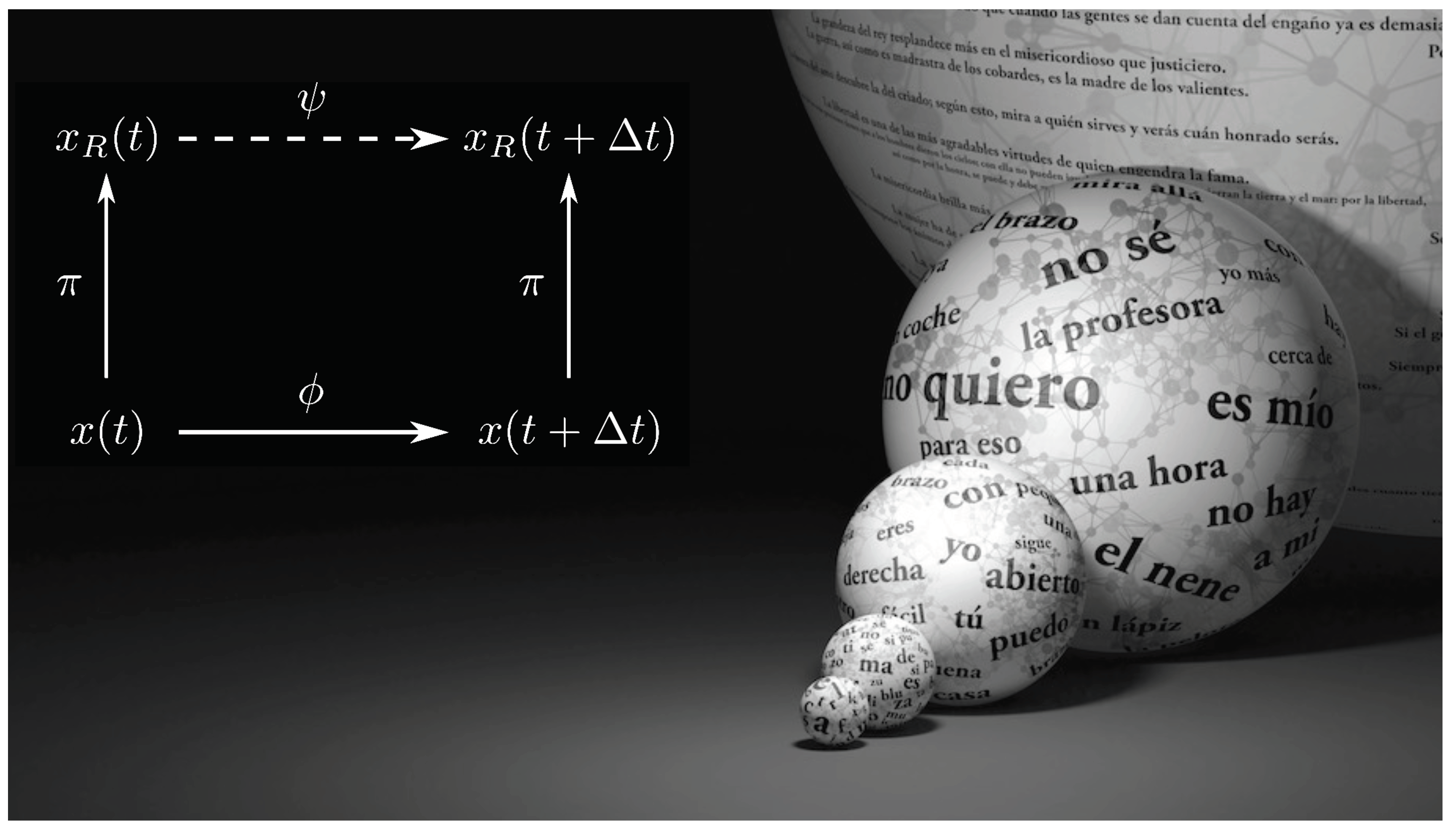
What is the “right” level of description for the faculty of human language? What would allow us to properly describe how it operates given the multiple scales involved—from letters and words to whole sentences? This nested character of language organization (
Figure 1) pervades the great challenge of understanding how it originated and how we could generate it artificially. The standard answer to these and similar questions is given by rules of thumb that have helped us, historically, to navigate the linguistic complexities. We have identified salient aspects (e.g., phonetics, formal grammars, etc.) to which whole fields are devoted. In adopting a level of description, we hope to encapsulate a helpful snippet of knowledge. To guide these choices we must broadly fulfill two goals: (i) the system under research (human language) must be somehow simplified and (ii) despite that simplification we must still capture as many relevant, predictive features about our system’s unfolding as possible. Some simplifications work better than others. In general, opting for a specific level does not mean that another one is not informative.
A successful approach to explore human language is through networks. Nodes of a language web can be letters, syllables, or words; links can represent co-occurrences, structural similarity, phonology, or syntactic or semantic relations [
1,
2,
3,
4,
5,
6,
7]. Are these different levels of description nested parsimoniously into each other? Or do sharp transitions exist that establish clear phenomenological realms? Most of the network-level topological analyses suggest potential paths to understand linguistic processing and hint at deeper features of language organization. However, the connection between different levels are seldom explored, with few exceptions based on purely topological patterns [
8]; or some ambitious attempts to integrate all linguistic scales from the evolutionary one to the production of phonemes [
9,
10].
In this paper, we present a methodology to tackle this problem in linguistics: When are different levels of description pertinent? When can we forgo some details and focus on others? For example, when do we need to attend to syntactic constraints, and when do we need to pay attention to phonology? How do the descriptions at different levels come together? This interplay can be far from trivial: note, e.g., how phonetics dictates the grammatical choice of the determiner form “a” or “an” in English. Similarly, phonetic choices with no grammatical consequence can evolve into rigid syntactic rules in the long term. Is the description at a higher level always grounded in all previous stages, or do descriptions exist that do not depend on details from other scales? Likely, these are not all or nothing question. Therefore, rather, how many details in a given description do we need to carry on to the next one?
To exemplify how these questions can be approached, we look at written corpora as symbolic series. There are many ways in which a written corpus can be considered a symbolic series. For example, we can study the succession of letters in a text. Then, the available vocabulary consists of all letters in the alphabet (often including punctuations marks):
Alternatively, we can consider words as indivisible. In such cases, our vocabulary (
) would consist of all entries in a dictionary. We can study even simpler symbolic dynamics, e.g., if we group together all words of each given grammatical class and consider words within a class equal to each other. From this point of view, we do not gain much by keeping explicit words in our corpora. We can just substitute each one by its grammatical class, for example,
After this, we can study the resulting series that have as symbols elements of the coarse-grained vocabulary:
Further abstractions are possible. For example, we can introduce a mapping that retains the difference between nouns and verbs, and groups all other words in an abstract third category:
It is fair to ask which of these descriptions are more useful, when to stop our abstractions, whether different levels define complementary or redundant aspects of language, etc. Each of these descriptions introduces an operation that maps the most fine-grained vocabulary into less detailed ones, for example,
To validate the accuracy of this mapping, we need a second element. At the most fundamental level, some unknown rules
exist. They are the ones connecting words to each other in real language and correspond to the generative mechanisms that we would like to unravel. At the level coarse-grained by a mapping
, we can propose a description
(
Figure 1) that captures how the less-detailed dynamics advance. How well can we recover the original series depends on our choices of
and
. Particularly good descriptions at different scales conform the answers to the questions raised above. The
and
mappings play roles similar to language grammar, i.e., sets of rules that tell us what words can follow each other. Some rules show up in actual corpora more often than others. Almost every sentence needs to deal with the Subject-Verb-Object (SVO) rule, but only seldom do we find all types of adjectives in a same phrase. If we would infer a grammar empirically by looking at English corpora, we could easily oversee that there is a rule for adjective order too. However, as it can be so easily missed, this might not be as important as SVO to understand how English works.
Here, we investigate grammars, or sets of rules, that are empirically derived from written corpora. We would like to study as many grammars as possible, and to evaluate numerically how well each of them works. In this approach, a wrong rule (e.g., one proposing that sentence order in English is VSO instead of SVO) would perform poorly and be readily discarded. It is more difficult to test descriptive grammars (e.g., a rule that dictates the adjective order), so instead we adopt abstract models that tell us the probability that classes of words follow each other. For example, in English, it is likely to find an adjective or a noun after a determiner, but it is unlikely to find a verb. Our approach is inspired by the information bottleneck method [
11,
12,
13,
14,
15], rate distortion theory [
16,
17], and similar techniques [
18,
19,
20,
21,
22]. In all these studies, arbitrary symbolic dynamics are divided into the observations up to a certain point,
, the dynamics from that point onward,
, and some coarse-grained model
R (which plays the role of our
and
combined) that attempts to conceptualize what has happened in
to predict what will happen in
. This scheme allows us to quantify mathematically how good is a choice of
. For example, it is usual to search for models
R that maximize the quantity:
for some
. The first term captures the information that the model carries about the observed dynamics
, the second term captures the information that the past dynamics carry about the future given the filter imposed by the model
R, and the metaparameter
weights the importance of each term towards the global optimization.
We will evaluate our probabilistic grammars in a similar (yet slightly different) fashion. For our method of choice, we first acknowledge that we are facing a Pareto, or Multi-Objective Optimization (MOO) problem [
23,
24,
25]. In this kind of problem we attempt to minimize or maximize different traits of the model simultaneously. Such efforts are often in conflict with each other. In our case, we want to make our models as simple as possible, but in that simplicity we ask that they retain as much of their predictive power as possible. We will quantify how different grammars perform in both these regards, and rank them accordingly. MOO problems rarely present global optima, i.e., we will not be able to find the best grammar. Instead, MOO solutions are usually embodied by Pareto-optimal trade-offs. These are collections of designs that cannot be improved in both optimization targets simultaneously. In our case these will be grammars that cannot be made simpler without losing some accuracy in their description of a text, or that cannot be made more accurate without making them more complicated.
The solutions to MOO problems are connected with statistical mechanics [
25,
26,
27,
28,
29]. The geometric representation of the optimal trade-off reveals phase transitions (similar to the phenomena of water turning into ice or evaporating promptly with slight variations of temperature around 0 or 100 degrees Celsius) and critical points. In our case, Pareto optimal grammars would give us a collection of linguistic descriptions that simultaneously optimize how simply language rules can become while retaining as much of their explanatory power as possible. The different grammars along a trade-off would become optimal descriptions at different levels, depending on how much detail we wish to track about a corpus. Positive (second order) phase transitions would indicate salient grammars that are adequate descriptions of a corpus at several scales. Negative (first order) phase transitions would indicate levels at which the optimal description of our language changes drastically and very suddenly between extreme sets of rules. Critical points would indicate the presence of somehow irreducible complexity in which different descriptions of a language become simultaneously necessary, and aspects included in one description are not provided by any other. Although critical points seem a worst-case scenario towards describing language, they are a favorite of statistical physics. Systems at a critical point often display a series of desirable characteristics, such as versatility, enhanced computational abilities, and optimal handling of memory [
30,
31,
32,
33,
34,
35,
36,
37,
38].
In
Section 2 we explain how we infer our
and
(i.e., our abstract “grammatical classes” and associated grammars), and the mathematical methods used to quantify how simple and accurate they are. In
Section 3, we present some preliminary results, always keeping in mind that this paper is an illustration of the intended methodology. More thorough implementations will follow in the future. In
Section 4, we reflect about the insights that we might win with these methods, how they could integrate more linguistic aspects, and how they could be adapted to deal with the complicated, hierarchical nature of language.
3. Results
Using the methodology described above, we have coarse-grained the words of a written corpus, first, into the 34 grammatical classes shown in
Table 1. This process is illustrated by Equation (
2). The resulting symbolic series was binarized to create samples akin to spin glasses, a well studied model from statistical mechanics that allows us to use powerful mathematical tools on our problem. This process was then repeated at several levels of coarse graining as words were further lumped into abstract grammatical categories (e.g., as in Equation (
4)). At each level of description, the inferred spin glass model plays the role of a grammar that constrains, in a probabilistic fashion, how word classes can follow each other in a text. These mathematical tools from spin glass theory allow us to test grammars from different description levels against each other as will become clear now.
In spin glasses, a collection of little magnets (or spins) is arranged in space. We say that a magnet is in state
if its north pole is pointing upwards and in state
if its pointing downwards (these are equivalent to the 1s and 0s in our word samples). Two of these little magnets interact through their magnetic fields. These fields build up a force that tends to align both spins in the same direction, whichever it is, just as two magnets in your hand try to fall along a specific direction with respect to each other. On top of this, the spins can interact with an external magnetic field—bringing in a much bigger magnet which orientation cannot be controlled. This external field tends to align the little spins along its fixed, preferred direction. Given the spin states
and
, the energy of their interaction with the external magnetic field and with each other can be written as
and
(with
) denote the strength of the interaction between the spins, and
and
denote the interaction of each spin with the external field. The terms
and
are also known as biases. If the spins are aligned with each other and with the external field, the resulting energy is the lowest possible. Each misalignment increases the energy of the system. In physics, states with less energy are more probable. Statistical mechanics allows us to write precisely the likelihood of finding this system in each of its four (
,
,
, and
) possible states:
where
is the inverse of the temperature. The term
is known as the partition function and is a normalizing factor that guarantees that the probability distribution in Equation (
16) is well defined.
Back to our text corpus in its binary representation, we know the empirical frequency
with which each of the possible spin configurations shows up—we just need to read it from our corpus. We can treat our collection of 0s and 1s as if they were
samples of a spin glass, and attempt to infer the
and
which (through a formula similar to Equation (
16)) more faithfully reproduce the observed sample frequencies. The superindex in
and
indicates that they will change with the level of coarse-graining. Inferring those
and
amounts to finding the MaxEnt model at that coarse-grained level. As advanced above, MaxEnt models are convenient because they are the models that introduce less extra hypotheses given some observations. In other words, if we infer the MaxEnt model for some
, any other model with the same coarse-graining would be introducing spurious hypotheses that are not suggested by the data. To infer MaxEnt models, we used Minimum Probability Flow Learning (MPFL [
50]), a fast and reliable method that infers the
given a sufficiently large sample.
Each grammatical class is represented by
spins at the
-th coarse-graining. This implies, as we know, that our samples consists of
spints. MPFL returns a matrix
of size
. This matrix embodies our abstract, probabilistic grammar (and plays the role of
in
Figure 1). Each entry
of this matrix tells us the interaction energy between the
k-th and
-th bits in a sample (with
). However, each grammatical class is represented not by one spin, but by a configuration of spins that has only one 1. To obtain the interaction energies between grammatical classes (rather than between spins), we need to compute
This energy in turn tells us the frequency with which we should observe each pair of words according to the model:
We inferred MaxEnt models for the more fine-grained level of description (
as given by the grammatical classes in
Table 1), as well as for every other intermediate level
.
Figure 2a shows the emerging spin-spin interactions for
, which consists of only 19 (versus the original 34) grammatical classes. This matrix presents a clear box structure:
The diagonal blocks ( and ) represent the interactions between all spins that define, separately, the first and second words in each sample. As our corpus becomes infinitely large, . These terms do not capture the interaction between grammatical classes. In the spin-glass analogy, they are equivalent to the interaction of each word with the external magnet that biases the presence of some grammatical classes over others. Such biases affect the frequencies with which individual classes show up, but not the frequency with which they are paired up. Therefore, the and are not giving us much syntactic information.
More interesting for us are the interaction terms stored in
and
. The inference method used guarantees that
. It is from these terms that we can compute the part of
(shown in
Figure 2b) that pertains to pairwise interaction alone (i.e., the energy of the spin system when we discount the interaction with the external field).
encodes the energy of two word classes when they are put next to each other in a text. The order in which words appear after each other is relevant, therefore that matrix is not symmetric. These energies reflect some of the rules of English. For example, the first row (labeled “E, M”) is a class that has lumped together the existential “there” (as in “there is” and “there are”) with all modal verbs. These tend to be followed by a verb in English, thus the matrix entry coding for
(marked in red) is much lower than most entries for any other
. The blue square encompasses verbs, nouns, and determiners. Although the differences there are very subtle, the energies reflect that it is more likely to see a noun after a determiner and not the other way around, and also that it is less likely to see a verb after a determiner.
It is not straightforward to compare all energies because they are affected by the raw frequency with which pairs of words show up in a text. In that sense, our corpus size might be sampling some pairings insufficiently so that their energies do not reflect proper English use. On the other hand, classes such as nouns, verbs, and determiners happen so often (and so often combined with each other) that they present very low energies as compared with other possible pairs. This makes the comparison more difficult by visual inspection.
It is possible to use to generate a synthetic text and evaluate its energy using the most fine-grained model . If the coarse-grained model retains a lot of the original structure, the generated text will fit gracefully in the rules dictated by —just as magnets falling into place. Such texts would present very low energy when evaluated by . If the coarse-grained model has erased much of the original structure, the synthetic text will present odd pairings. These would feel similar to magnets that we are forcing into a wrong disposition, therefore resulting in a large energy when is used. In other words, this energy reflects how accurate each coarse-grained model is.
That accuracy is one of the targets in our MOO problem, in which we attempt to retain as much information as possible with models as simple as possible. To quantify that second target, simplicity, we turn to entropy. The simplest model possible generates words that fall in either class of randomly and uniformly, thus presenting the largest entropy possible. More complex models, in their attempt to remain accurate, introduce constraints as to how the words in the coarse-grained model must be mapped back into the classes available in . That operation would be the reverse of . This reverse mapping, however, cannot be undone without error because the coarse-graining erases information. Entropy measures the amount of information that has been erased, and therefore how simple the model has been made.
Figure 3b shows the energy
and entropy
for synthetic texts generated with the whole range of coarse-grainings explored. In terms of Pareto optimality, we expect our models to have as low an energy as possible while having the largest entropy compatible with each energy—just as thermodynamic systems do. Such models would simultaneously optimize their simplicity and accuracy. Within the sample, some of these models are Pareto dominated (crosses in
Figure 3b) by some others. This means that for each of those models at least some other one exists that is simpler and more accurate at the same time. These models are suboptimal regarding both optimization targets, so we do not need to bother with them.The non-dominated ones (marked by circles in
Figure 3b) capture better descriptions in both senses (accuracy and simplicity). They are such that we cannot move from one to another without improving an optimization target and worsening the other. They embody the optimal trade-off possible (of course, limited by all the approximations made in this paper), and we cannot choose a model over the others without introducing some degree of artificial preference either for simplicity or accuracy.
In statistical mechanics the energy and entropy of a system are brought together by the free energy:
Here,
plays a role akin to a temperature and
plays the role of its inverse. We noted
to indicate that these temperature and inverse temperature are different from the ones in Equation (
19). Those temperatures control how often a word shows up given a model, whereas
controls how appropriate each level of description is. When
is low (and
is large), a minimum free energy in Equation (
21) is attained by maximizing the entropy rather than minimizing the energy. This is, low
selects for simpler descriptions. When
is large (and
is small), we prefer models with lower energy, i.e., higher accuracy.
By varying
we visit the range of models available, i.e., we visit the collection of Pareto optimal grammars (circles in
Figure 3b). In statistical mechanics, by varying the temperature of a system we visit a series of states of matter (this is, we put, e.g., a glass of water at different temperatures and observe how its volume and pressure change). At some relevant points, called phase transitions, the states of matter change radically, e.g., water freezes swiftly at 0 degrees Celsius, and evaporates right at 100 degrees Celsius. The geometry of Pareto optimal states of matter tells us when such transitions occur [
25,
26,
27,
28,
29].
Similarly, the geometric disposition of Pareto optimal models in
Figure 3b tells us when a drastic change in our best description is needed as we vary
. Relevant phase transitions are given by cavities and salient points along the Pareto optimal solutions. In the first approach, we observe several cavities. More interestingly, perhaps, is the possibility that our Pareto optimal models might fall along a straight line; one has been added as a guideline in
Figure 3b. Although there are obvious deviations from it, such description might be feasible at large. Straight lines in this plot are interesting because they indicate the existence of special critical points [
28,
37,
46,
47,
48]. In the next section, we discuss what criticality might mean in this context.
4. Discussion
In this paper, we study how different hierarchical levels in the description of human language are entangled with each other. Our work is currently at a preliminary stage, and this manuscript aims at presenting overall goals and a possible methodological way to tackle relevant questions. Some interesting results are presented as an illustration and discussed in this section to exemplify the kind of debate that this line of research can spark.
Our work puts forward a rigorous and systematic framework to tackle the questions introduced above, namely, what levels of description are relevant to understand human language and how do these different descriptions interact with each other. Historically, we have answered these questions guided by intuition. Some aspects of language are so salient that they demand a sub-field of their own. Although this complexity and interconnectedness is widely acknowledged, its study is still fairly compartmentalized. The portray of language as a multilayered network system is a recent exception [
8], as it is the notable and lasting effort by Christiansen et al. [
9,
10] to link all scales of language production, development, and evolution in a unified frame.
We generated a collection of models that describe a written English corpus. These models trade optimally a decreasing level of accuracy by increasing simplicity. By doing so, they gradually lose track of variables involved in the description at more detailed levels. For example, as we saw above, the existential “there” is merged with modal verbs. Indeed, these two classes were lumped together before the distinction between all other verbs was erased. Although those grammatical classes are conceptually different, our blind methodology found convenient to merge them earlier in order to elaborate more efficient compact grammars.
Remaining as accurate as possible while becoming as simple as possible is a multi-objective optimization problem. The conflicting targets are captured by the energy and entropy that artificial texts generated by a coarse-grained model have when evaluated at the most accurate level of description. We could have quantified these targets in other ways (e.g., counting the number of grammatical classes to quantify complexity, and measuring similarity between synthetic and real texts for accuracy). Those alternative choices should be explored systematically in the future to understand which options are more informative. Our choices, however, make our results easy to interpret in physical terms. For example, improbable (unnatural) texts have high energies in any good model.
The grammars that optimally trade between accuracy (low energy) and simplicity (high entropy) conform the Pareto front (i.e., the solution) of the MOO problem. Its shape in the energy-entropy plane (
Figure 3) is linked to phase transitions [
25,
26,
27,
28,
29]. According to this framework, we do not find evidence of a positive (second order) phase transition. What could such a transition imply for our system? The presence of a positive phase transition in our data would suggest the existence of a salient level of description capable of capturing a large amount of linguistic structure in relatively simple terms. For example, if a unique grammatical rule would serve to connect words together disregarding of the grammatical classes in which we have split our vocabulary. We would expect that to be the case, e.g., if a single master rule such as merge would serve to generate all the complexity of human language without further constraints arising. This does not seem to be the case. However, this does not rule out the existence of the relevant merge operation, nor does it deny its possible fundamental role. Indeed, Chomsky proposes that merge is the fundamental operation of syntax, but that it leaves the creative process of language underconstrained [
51,
52,
53]. As a result, actual implementations (i.e., real languages) see a plethora of further complexities arising in a phenomena akin to symmetry breaking.
The presence of a negative (first order) phase transition would acknowledge several salient levels of description needed to understand human language. These salient descriptions would furthermore present an important gap separating them. This would indicate that discrete approaches would be possible to describe language without missing any detail by ignoring the intermediate possibilities. If that were the case, we would still need to analyze the emerging models and look at similarities between them to understand whether both models capture a same core phenomenology at two relevant (yet distant) scales; or whether each model focuses on a specific, complementary aspect that the other description has no saying about. Some elements in
Figure 3b are compatible with this kind of phase transition.
However, the disposition of several Pareto optimal grammars along a seemingly straight line rather suggests the existence of a special kind of critical phenomenon [
28,
37,
46,
47,
48]. Criticality is a worst-case scenario in terms of description. It implies that there is no trivial model, nor couple of models, nor relatively small collection that can capture the whole of linguistic phenomenology at any level. A degenerate number of descriptions is simultaneously necessary, and elements trivial in a level can become cornerstones of another. Also, potentially, constraints imposed by a linguistic domain (e.g., phonology) can penetrate all the way and alter the operating rules of other domains (e.g., syntax or semantics). We can list examples of how this happens in several tongues (such as the case of determiners “a” and ‘an’ in English mentioned above). The kind of criticality suggested by our results would indicate that such intrusions are the norm rather than the exception. Note that this opportunistic view of grammar appears compatible with Christiansen’s thesis that language evolved, as an interface, to make itself useful to our species, necessarily exploiting all kinds of hacks along its way [
9].
Zipf’s law is a notable distribution in linguistics [
54,
55]. It states that the
n-th most abundant word in a text shows up with a frequency that is inversely proportional to that word’s rank (i.e.,
n). The presence of this distribution in linguistic corpora has been linked to an optimal balance between communicative tensions [
54,
56,
57]. It has also been proved mathematically that Zipf’s law is an unavoidable feature of open-ended evolving systems [
58]. Languages and linguistic creativity are candidates to present open-ended evolution. Could this open-endedness be reflected also in the diversity of grammatical rules that form a language? Could we expect to find a power-law in the distribution of word combinations with a given energy? If that were the case, Bialek et al. [
37,
47] proved mathematically that the relationship between energy and entropy of such grammars must be linear and therefore critical. In other words, our observation of criticality in this work, if confirmed, would be a strong hint (yet not sufficient) that the relevant Zipf distribution may also be lurking behind grammars derived empirically from written corpora.
Numerous simplifications were introduced to produce the preliminary results in this paper. We started our analysis with words that have already been coarse-grained into 34 grammatical classes, barring the emergence of further intermediate categories dictated, e.g., by semantic use. We know that semantic considerations can condition combinations of words, such as what verbs can be applied to what kinds of agents [
59]. The choice of words as units (instead of letters or syllables) is another limiting factor. Words are symbols whose meanings do not depend on physical correlates with the objects signified [
60]. In that sense, their association to their constituent letters and phonems is arbitrary. Their meaning is truly emergent and not rooted in their parts. Introducing letters, syllables, and phonetics in our analysis might reveal and allow us to capture that true emergence.
To do this it might be necessary to work with hierarchical models that allow correlations beyond the next and previous words considered here. This kind of hierarchy, in general, is a critical aspect of language [
53] that our approach should capture in due time. We have excluded it in this work to attain preliminary results in a reasonable time. Although hierarchical models are likely to be more demanding (in computational terms), they can be parsimoniously incorporated in our framework. A possibility is to use epsilon machines [
61,
62,
63], which naturally lump together pieces of symbolic dynamics to find out causal states. These causal states act as shielding units that advance a symbolic dynamics in a uniquely determined way—just like phrases or sentences provide a sense of closure at their end, and direct the future of a text in new directions.


