1. Introduction
The interplay between inequalities and information theory has a rich history, with notable examples including the relationship between the Brunn–Minkowski inequality and the entropy power inequality as well as the matrix determinant inequalities obtained from differential entropy [
1]. In this paper, the focus is on a “two-moment” inequality that provides an upper bound on the integral of the
rth power of a function. Specifically, if
f is a nonnegative function defined on
and
are real numbers satisfying
and
, then
where the best possible constant
is given exactly; see Propositions 2 and 3 ahead. The one-dimensional version of this inequality is a special case of the classical Carlson–Levin inequality [
2,
3,
4], and the multidimensional version is a special case of a result presented by Barza et al. [
5]. The particular formulation of the inequality used in this paper was derived independently in [
6], where the proof follows from a direct application of Hölder’s inequality and Jensen’s inequality.
In the context of information theory and statistics, a useful property of the two-moment inequality is that it provides a bound on a nonlinear functional, namely the
r-quasi-norm
, in terms of integrals that are linear in
f. Consequently, this inequality is well suited to settings where
f is a mixture of simple functions whose moments can be evaluated. We note that this reliance on moments to bound a nonlinear functional is closely related to bounds obtained from variational characterizations such as the Donsker–Varadhan representation of Kullback divergence [
7] and its generalizations to Rényi divergence [
8,
9].
The first application considered in this paper concerns the relationship between the entropy of a probability measure and its moments. This relationship is fundamental to the principle of maximum entropy, which originated in statistical physics and has since been applied to statistical inference problems [
10]. It also plays a prominent role in information theory and estimation theory where the fact that the Gaussian distribution maximizes differential entropy under second moment constraints ([
11], [Theorem 8.6.5]) plays a prominent role. Moment–entropy inequalities for Rényi entropy were studied in a series of works by Lutwak et al. [
12,
13,
14], as well as related works by Costa et al. [
15,
16] and Johonson and Vignat [
17], in which it is shown that, under a single moment constraint, Rényi entropy is maximized by a family of generalized Gaussian distributions. The connection between these moment–entropy inequalities and the Carlson–Levin inequality was noted recently by Nguyen [
18].
In this direction, one of the contributions of this paper is a new family of moment–entropy inequalities. This family of inequalities follows from applying Inequality (
1) in the setting where
f is a probability density function, and thus there is a one-to-one correspondence between the integral of the
rth power and the Rényi entropy of order
r. In the special case where one of the moments is the zeroth moment, this approach recovers the moment–entropy inequalities given in previous work. More generally, the additional flexibility provided by considering two different moments can lead to stronger results. For example, in Proposition 6, it is shown that if
f is the standard Gaussian density function defined on
, then the difference between the Rényi entropy and the upper bound given by the two-moment inequality (equivalently, the ratio between the left- and right-hand sides of (
1)) is bounded uniformly with respect to
n under the following specification of the moments:
Conversely, if one of the moments is restricted to be equal to zero, as is the case in the usual moment–entropy inequalities, then the difference between the Rényi entropy and the upper bound diverges with
n.
The second application considered in this paper is the problem of bounding mutual information. In conjunction with Fano’s inequality and its extensions, bounds on mutual information play a prominent role in establishing minimax rates of statistical estimation [
19] as well as the information-theoretic limits of detection in high-dimensional settings [
20]. In many cases, one of the technical challenges is to provide conditions under which the dependence between the observations and an underlying signal or model parameters converges to zero in the limit of high dimension.
This paper introduces a new method for bounding mutual information, which can be described as follows. Let
be a probability measure on
such that
and
have densities
and
with respect to the Lebesgue measure on
. We begin by showing that the mutual information between
X and
Y satisfies the upper bound
where
is the variance of
; see Proposition 8 ahead. In view of (
3), an application of the two-moment Inequality (
1) with
leads to an upper bound with respect to the moments of the variance of the density:
where this expression is evaluated at
with
. A useful property of this bound is that the integrated variance is quadratic in
, and thus Expression (
4) can be evaluated by swapping the integration over
y and with the expectation of over two independent copies of
X. For example, when
is a Gaussian scale mixture, this approach provides closed-form upper bounds in terms of the moments of the Gaussian density. An early version of this technique is used to prove Gaussian approximations for random projections [
21] arising in the analysis of a random linear estimation problem appearing in wireless communications and compressed sensing [
22,
23].
2. Moment Inequalities
Let
be the space of Lebesgue measurable functions from
S to
whose
pth power is absolutely integrable, and for
, define
Recall that
is a norm for
but only a quasi-norm for
because it does not satisfy the triangle inequality. The
sth moment of
f is defined as
where
denotes the standard Euclidean norm on vectors.
The two-moment Inequality (
1) can be derived straightforwardly using the following argument. For
, the mapping
is concave on the subset of nonnegative functions and admits the variational representation
where
is the Hölder conjugate of
r. Consequently, each
leads to an upper bound on
. For example, if
f has bounded support
S, choosing
g to be the indicator function of
S leads to the basic inequality
. The upper bound on
given in Inequality (
1) can be obtained by restricting the minimum in Expression (
5) to the parametric class of functions of the form
with
and then optimizing over the parameters
. Here, the constraints on
are necessary and sufficient to ensure that
.
In the following sections, we provide a more detailed derivation, starting with the problem of maximizing
under multiple moment constraints and then specializing to the case of two moments. For a detailed account of the history of the Carlson type inequalities as well as some further extensions, see [
4].
2.1. Multiple Moments
Consider the following optimization problem:
For
, this is a convex optimization problem because
is concave and the moment constraints are linear. By standard theory in convex optimization (e.g., [
24]), it can be shown that if the problem is feasible and the maximum is finite, then the maximizer has the form
The parameters
are nonnegative and the
ith moment constraint holds with equality for all
i such that
is strictly positive—that is,
. Consequently, the maximum can be expressed in terms of a linear combination of the moments:
For the purposes of this paper, it is useful to consider a relative inequality in terms of the moments of the function itself. Given a number
and vectors
and
, the function
is defined according to
if the integral exists. Otherwise,
is defined to be positive infinity. It can be verified that
is finite provided that there exists
such that
and
are strictly positive and
.
The following result can be viewed as a consequence of the constrained optimization problem described above. We provide a different and very simple proof that depends only on Hölder’s inequality.
Proposition 1. Let f be a nonnegative Lebesgue measurable function defined on the positive reals . For any number and vectors and , we have Proof. Let
. Then, we have
where the second step is Hölder’s inequality with conjugate exponents
and
. □
2.2. Two Moments
For
, the beta function
and gamma function
are given by
and satisfy the relation
,
. To lighten the notation, we define the normalized beta function
Properties of these functions are provided in
Appendix A.
The next result follows from Proposition 1 for the case of two moments.
Proposition 2. Let f be a nonnegative Lebesgue measurable function defined on . For any numbers with and ,where andwhere is defined in Equation (6). Proof. Letting
and
with
, we have
Making the change of variable
leads to
where
and
and the second step follows from recognizing the integral representation of the beta function given in Equation (
A3). Therefore, by Proposition 1, the inequality
holds for all
. Evaluating this inequality with
leads to the stated result. □
The special case
admits the simplified expression
where we have used Euler’s reflection formula for the beta function ([
25], [Theorem 1.2.1]).
Next, we consider an extension of Proposition 2 for functions defined on
. Given any measurable subset
S of
, we define
where
is the
n-dimensional Euclidean ball of radius one and
The function
is proportional to the surface measure of the projection of
S on the Euclidean sphere and satisfies
for all
. Note that
and
.
Proposition 3. Let f be a nonnegative Lebesgue measurable function defined on a subset S of . For any numbers with and ,where and is given by Equation (7). Proof. Let
f be extended to
using the rule
for all
x outside of
S and let
be defined according to
where
is the Euclidean sphere of radius one and
is the surface measure of the sphere. In the following, we will show that
Then, the stated inequality then follows from applying Proposition 2 to the function
g.
To prove Inequality (
11), we begin with a transformation into polar coordinates:
Letting
denote the indicator function of the set
, the integral over the sphere can be bounded using:
where: (a) follows from Hölder’s inequality with conjugate exponents
and
, and (b) follows from the definition of
g and the fact that
Plugging Inequality (
14) back into Equation (
13) and then making the change of variable
yields
The proof of Equation (12) follows along similar lines. We have
where (a) follows from a transformation into polar coordinates and (b) follows from the change of variable
.
Having established Inequality (
11) and Equation (12), an application of Proposition 2 completes the proof. □
3. Rényi Entropy Bounds
Let
X be a random vector that has a density
with respect to the Lebesgue measure on
. The differential Rényi entropy of order
is defined according to [
11]:
Throughout this paper, it is assumed that the logarithm is defined with respect to the natural base and entropy is measured in nats. The Rényi entropy is continuous and nonincreasing in
r. If the support set
has finite measure, then the limit as
r converges to zero is given by
. If the support does not have finite measure, then
increases to infinity as
r decreases to zero. The case
is given by the Shannon differential entropy:
Given a random variable
X that is not identical to zero and numbers
with
and
, we define the function
where
.
The next result, which follows directly from Proposition 3, provides an upper bound on the Rényi entropy.
Proposition 4. Let X be a random vector with a density on . For any numbers with and , the Rényi entropy satisfieswhere is defined in Equation (9) and is defined in Equation (7). Proof. This result follows immediately from Proposition 3 and the definition of Rényi entropy. □
The relationship between Proposition 4 and previous results depends on whether the moment p is equal to zero:
One-moment inequalities: If
, then there exists a distribution such that Inequality (
15) holds with equality. This is because the zero-moment constraint ensures that the function that maximizes the Rényi entropy integrates to one. In this case, Proposition 4 is equivalent to previous results that focused on distributions that maximize Rényi entropy subject to a single moment constraint [
12,
13,
15]. With some abuse of terminology, we refer to these bounds as one-moment inequalities. (A more accurate name would be two-moment inequalities under the constraint that one of the moments is the zeroth moment.)
Two-moment inequalities: If
, then the right-hand side of Inequality (
15) corresponds to the Rényi entropy of a nonnegative function that might not integrate to one. Nevertheless, the expression provides an upper bound on the Rényi entropy for any density with the same moments. We refer to the bounds obtained using a general pair
as two-moment inequalities.
The contribution of two-moment inequalities is that they lead to tighter bounds. To quantify the tightness, we define
to be the gap between the right-hand side and left-hand side of Inequality (
15) corresponding to the pair
—that is,
The gaps corresponding to the optimal two-moment and one-moment inequalities are defined according to
3.1. Some Consequences of These Bounds
By Lyapunov’s inequality, the mapping
is nondecreasing on
, and thus
In other words, the case
provides an upper bound on
for nonnegative
p. Alternatively, we also have the lower bound
which follows from the convexity of
.
A useful property of
is that it is additive with respect to the product of independent random variables. Specifically, if
X and
Y are independent, then
One consequence is that multiplication by a bounded random variable cannot increase the Rényi entropy by an amount that exceeds the gap of the two-moment inequality with nonnegative moments.
Proposition 5. Let Y be a random vector on with finite Rényi entropy of order , and let X be an independent random variable that satisfies . Then,for all . Proof. Let
and let
and
denote the support sets of
Z and
Y, respectively. The assumption that
X is nonnegative means that
. We have
where (a) follows from Proposition 4, (b) follows from Equation (
18) and the definition of
, and (c) follows from Inequality (
16) and the assumption
. Finally, recalling that
completes the proof. □
3.2. Example with Log-Normal Distribution
If
, then the random variable
has a log-normal distribution with parameters
. The Rényi entropy is given by
and the logarithm of the
sth moment is given by
With a bit of work, it can be shown that the gap of the optimal two-moment inequality does not depend on the parameters
and is given by
The details of this derivation are given in
Appendix B.1. Meanwhile, the gap of the optimal one-moment inequality is given by
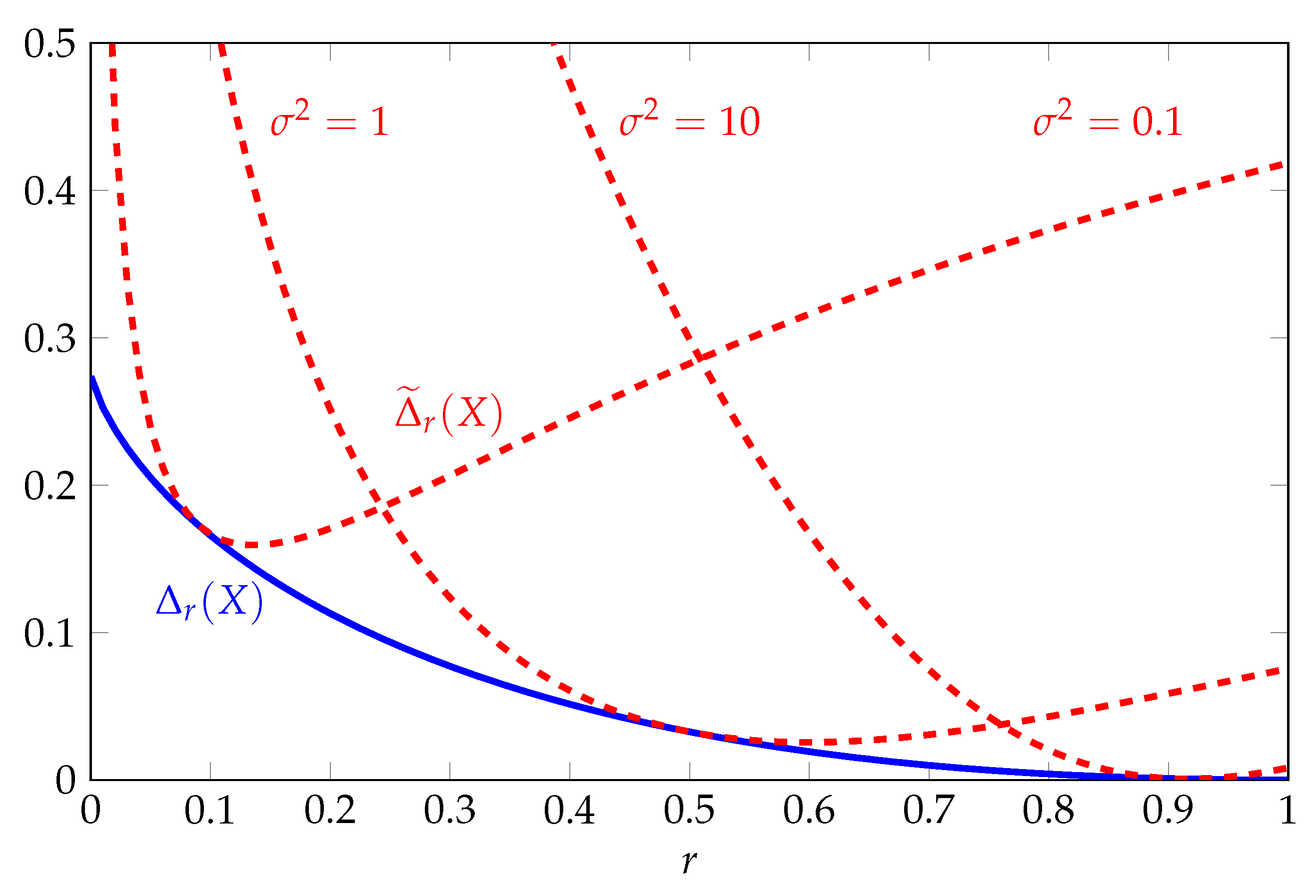
The functions
and
are illustrated in
Figure 1 as a function of
r for various
. The function
is bounded uniformly with respect to
r and converges to zero as
r increases to one. The tightness of the two-moment inequality in this regime follows from the fact that the log-normal distribution maximizes Shannon entropy subject to a constraint on
. By contrast, the function
varies with the parameter
. For any fixed
, it can be shown that
increases to infinity if
converges to zero or infinity.
3.3. Example with Multivariate Gaussian Distribution
Next, we consider the case where
is an
n-dimensional Gaussian vector with mean zero and identity covariance. The Rényi entropy is given by
and the
sth moment of the magnitude
is given by
The next result shows that as the dimension
n increases, the gap of the optimal two-moment inequality converges to the gap for the log-normal distribution. Moreover, for each
, the following choice of moments is optimal in the large-
n limit:
The proof is given in
Appendix B.3.
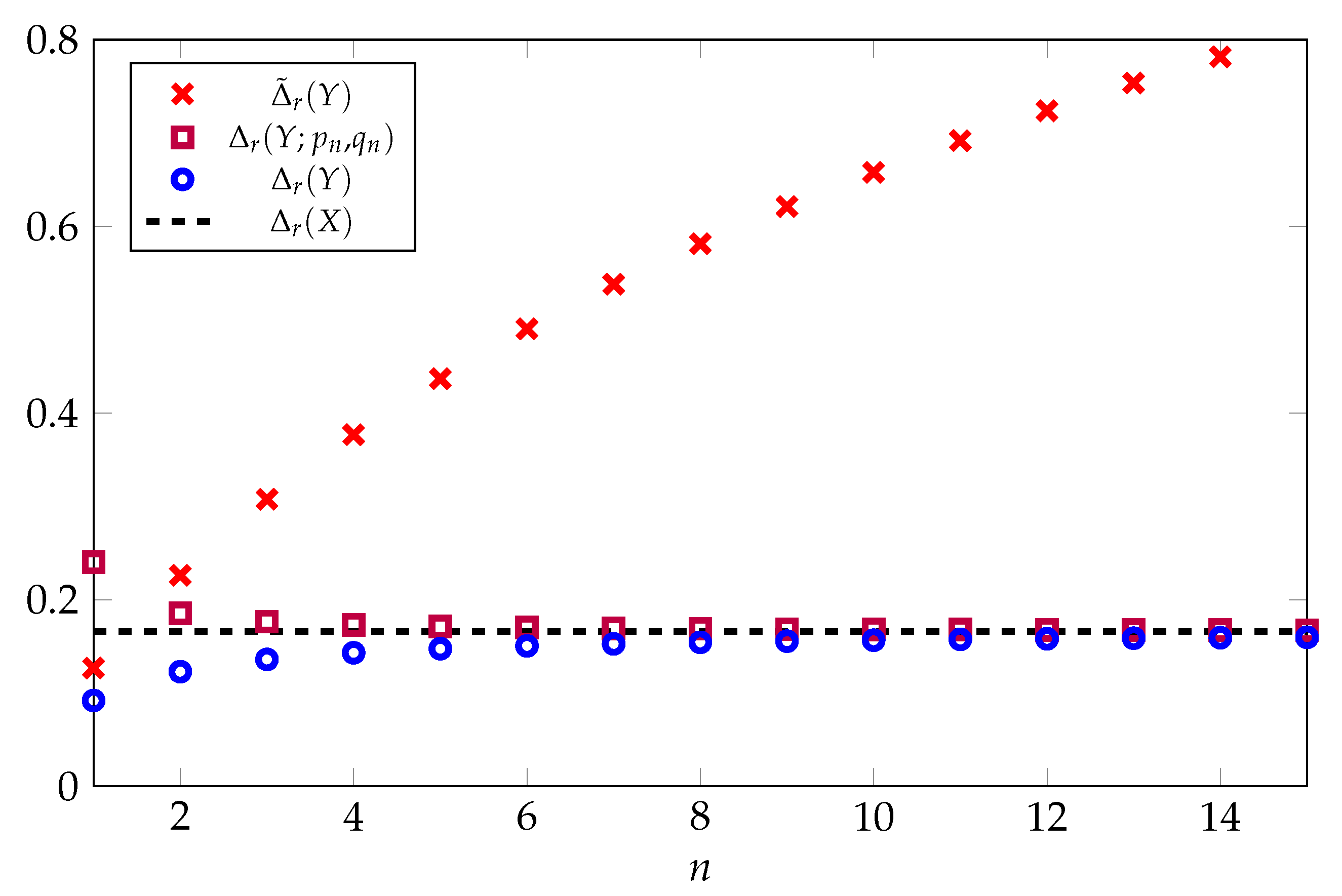
Proposition 6. If , then, for each ,where X has a log-normal distribution and are given by (21). Figure 2 provides a comparison of
,
, and
as a function of
n for
. Here, we see that both
and
converge rapidly to the asymptotic limit given by the gap of the log-normal distribution. By contrast, the gap of the optimal one-moment inequality
increases without bound.
3.4. Inequalities for Differential Entropy
Proposition 4 can also be used to recover some known inequalities for differential entropy by considering the limiting behavior as
r converges to one. For example, it is well known that the differential entropy of an
n-dimensional random vector
X with finite second moment satisfies
with equality if and only if the entries of
X are i.i.d. zero-mean Gaussian. A generalization of this result in terms of an arbitrary positive moment is given by
for all
. Note that Inequality (
22) corresponds to the case
.
Inequality (
23) can be proved as an immediate consequence of Proposition 4 and the fact that
is nonincreasing in
r. Using properties of the beta function given in
Appendix A, it is straightforward to verify that
Combining this result with Proposition 4 and Inequality (
16) leads to
Using Inequality (
10) and making the substitution
leads to Inequality (
23).
Another example follows from the fact that the log-normal distribution maximizes the differential entropy of a positive random variable
X subject to constraints on the mean and variance of
, and hence
with equality if and only if
X is log-normal. In
Appendix B.4, it is shown how this inequality can be proved using our two-moment inequalities by studying the behavior as both
p and
q converge to zero as
r increases to one.


