1. Introduction
Much below the linear critical Reynolds number of the parabolic channel flow, transition to turbulence can occur under finite-amplitude perturbations, i.e., via a subcritical transition. Numerous studies have established that turbulence takes the form of discrete turbulent bands that are oblique to the streamwise direction, interspersed with laminar flow, at transitional Reynolds numbers [
1,
2,
3,
4,
5,
6,
7,
8,
9,
10]. Similar banded turbulent structures have also been observed in other quasi-two-dimensional flows, i.e., systems with one confined dimension and two extended dimensions, such as plane Couette [
11,
12,
13], Taylor Couette [
14,
15], annular pipe [
16] and Wallefe flows [
17]. Therefore, the coexistence of laminar and turbulent states in the form of banded turbulent structures is a common feature of turbulence at transitional Reynolds numbers of a broad variety of shear flows. Recent investigations into these structures have greatly advanced the understanding of the subcritical transition in these flows [
10,
18]. In the following discussion, for channel flow, the streamwise, wall-normal and spanwise directions are denoted as
x,
y and
z, respectively, time is denoted as
t and the half-channel-height as
h. The flow is assumed driven by a constant volume flux and the Reynolds number is defined as
, where
is the centerline velocity of the unperturbed parabolic flow and
the kinematic viscosity of the fluid.
The first observation and many numerical studies of turbulent bands in channel flow were performed by numerical simulations in relatively small computational domains, either normal or tilted, in which the structure, kinematics and dynamics of turbulent bands are rather restrained [
1,
2,
4,
19,
20]. Particularly, narrow tilted domains force turbulent bands to be parallel to the narrow edge, which practically assumes infinitely long bands in combination with periodic boundary conditions. Nevertheless, this greatly reduces the computational cost and allows studying the kinematics and dynamics of bands over large time scales [
9,
20] and offers conveniences for studying the mean flow and wavelength of the band pattern [
4,
10]. In a domain tilted by
, Tuckerman et al. [
4] reported that turbulent bands propagate approximately at the bulk speed of the flow, with a slight decreasing trend with the Reynolds number (the speed crosses the bulk speed at
). In a similar approach as Avila et al. [
21] for pipe flow and Shi et al. [
22] for plane Couette flow, Gomé et al. [
20] also showed finite lifetime and splitting nature of bands and determined the on-set of sustained turbulence in channel flow to be at
by balancing the super-exponential decay and splitting processes, in a domain also tilted by
. The subcritical transition to turbulence in plane Couette flow in tilted domains has been concluded to fall in the universality class of directed percolation [
23] and the work of Gomé et al. [
20] seems to suggest the same transition scenario in channel flow. However, the imposed tilt angle of the domain seems to affect the statistical results. For example, the simulations in a domain tilted by
[
9] showed very different lifetimes of bands from the results of Gomé et al. [
20]. Specifically, the former reported that turbulent bands are sustained at
, whereas the latter suggested that in fact the lifetime stays finite and is below 200 time units at
. The effect of the imposed tilt angle has not been thoroughly investigated. Besides, the usual narrow tilted domain only allows multiple bands to form parallel band pattern, i.e., bands are forced to take the same orientation.
Large domains pose a lesser restriction on turbulent bands. In recent years, a few studies have been dedicated to turbulent bands in large normal domains in experiments [
3,
9] and simulations [
5,
6,
7,
8,
24,
25]. If the domain is large enough, given a proper localized perturbation, turbulence elongates obliquely with respect to the streamwise direction and forms a fully localized band (localized both in its length direction and in its width direction). The existence of the two ends of the band adds further complexity to the flow. Paranjape [
9] reported in experiment that at
, a turbulent band shrinks and will decay so that the flow will relaminarize in the end, because the growth at the downstream end (referred to as the head hereafter) is slower than the decay at the upstream end (referred to as the tail hereafter). At higher Reynolds numbers, a turbulent band becomes sustained because the growth at the head outperforms the decay at the tail and will grow in length. Numerical studies [
6,
7,
24] agree with the experiments. Therefore, it has been confirmed that the growth of a band is unidirectional, driven by the head [
7,
8,
9,
24]. Because streaks decay at the tail and are generated at the head, an individual band undergoes a spanwise shift as a whole, aside from being advected in the streamwise direction. Shimizu and Manneville [
8] mentioned that the spanwise drift speed is 0.1 and Xiao and Song [
24] reported a close value of 0.08. Noticing the periodic streak generation at the head, Kanazawa [
7] and Xiao and Song [
24], respectively, proposed mechanisms behind the wave generation at the head, which are discussed in more detail below.
In fact, it was found that the length of a band does not grow infinitely. The length ‘at equilibrium’ of a band at
was shown to be about 300
h and the length seems to increase with
[
7]. As the length is sufficiently large, the fast decay of the tail limits the growth, and splitting may occur with a daughter band nucleated. At relatively low Reynolds numbers, the splitting is longitudinal, i.e., the daughter band is parallel to the mother band. As Reynolds number increases (
), transverse splitting (or branching) can also occur, nucleating daughter bands with the opposite tilt direction such that the flow pattern becomes two-sided (the criss-cross pattern) [
8,
9]. However, the study of the splitting of bands and the underlying mechanism is still rare.
In the presence of multiple bands, given that bands have a spanwise shift speed as a whole and can grow in length, close bands with opposite orientations may collide. Even parallel bands, when located sufficiently close to each other, were shown to interact also [
6,
8]. The dynamics of individual bands and the interaction between bands determine the pattern that bands can form and therefore, determine the statistical aspect of the transition to turbulence [
8]. Using unprecedented large domain and simulating up to very large times (up to
time units), Shimizu and Manneville [
8] showed that turbulent bands can only form one-sided (parallel) pattern at low Reynolds numbers (
), breaking the spanwise symmetry, which is restored only at higher Reynolds numbers. Directed percolation was found to reasonably well describe the transition process toward featureless turbulence at further higher Reynolds numbers, as also proposed by Sano and Tamai [
26] in experiments. Interestingly, the one-sided pattern of turbulent bands at lowest Reynolds numbers seems to justify the use of tilted domain in which bands are forced to be parallel, although the tilt angle was shown about
–
below
[
6,
7,
8,
9] rather than
as used in some studies [
4,
20].
Although a great advancement in the understanding of turbulent bands has been made in recent studies, many problems even for individual turbulent bands have not been well understood, for example the mechanisms underlying the growth of bands at the head and the decay at the tail, the tilt angle selection and the self-sustaining mechanism of the bulk of turbulent bands. We discuss some of these problems in this paper.
4. Tilt Angle of Turbulent Bands
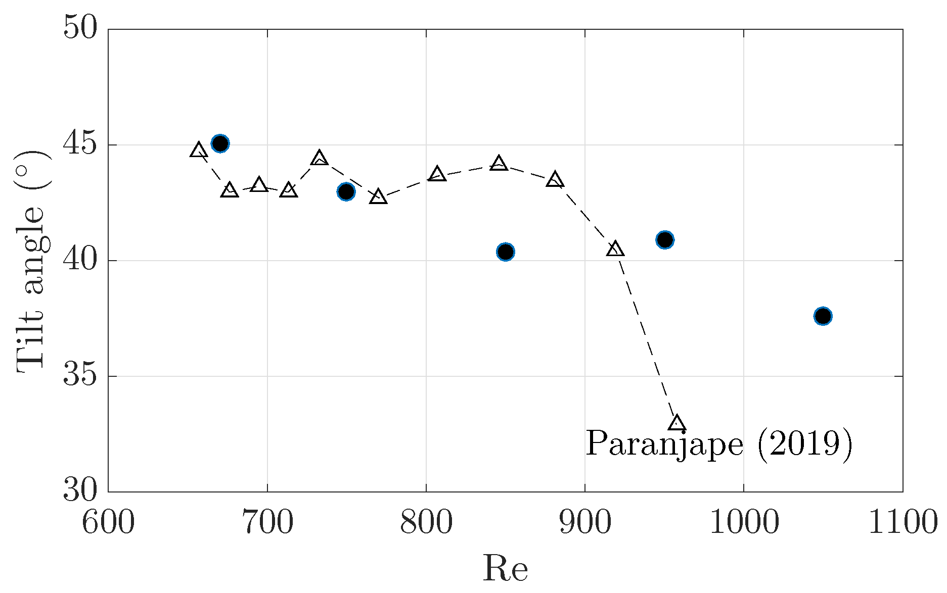
The tilt angle of turbulent bands at
was reported in experiments by Paranjape [
9]. Their measurements showed that the angle stays nearly constant close to
below
and decreases to approximately
above
. The decreasing trend was also reported by Shimizu and Manneville [
8]. A few numerical studies also reported the tilt angle at some Reynolds numbers; for example, Kanazawa [
7] reported
at
, Tao et al. [
6] reported approximately
at
and Xiao and Song [
24] reported an angle of about
at
, which are lower than but close to the experimental results of Paranjape [
9]. The small difference may be attributed to the periodic boundary condition used in simulations and to the specific methods of quantifying the tilt angle.
However, the mechanism underlying the tilt angle selection is still not well-understood. Prior studies simply measured the tilt angle by considering the entire band as a tilted object based on image processing or in similar manners [
6,
9]. Differently, here we propose that the tilt angle should be more fundamentally determined by the propagation speed of the head and the advection speed of the streaks inside the bulk. More specifically, the speed of the streaks inside the bulk relative to the head should determine the tilt angle of the band. Based on our measurements shown in
Figure 2 and
Figure 7, we calculated the tilt angle of the band as
The result is shown in
Figure 8. Our calculations agree well with the experimental result of Paranjape [
9] below
. However, at
, our calculation appears to be much higher than their measurement: our calculation gives
for
, whereas it was estimated to be around
in experiments. Nevertheless, our calculation gives the decreasing trend in the tilt angle as
is increased to around
and above.
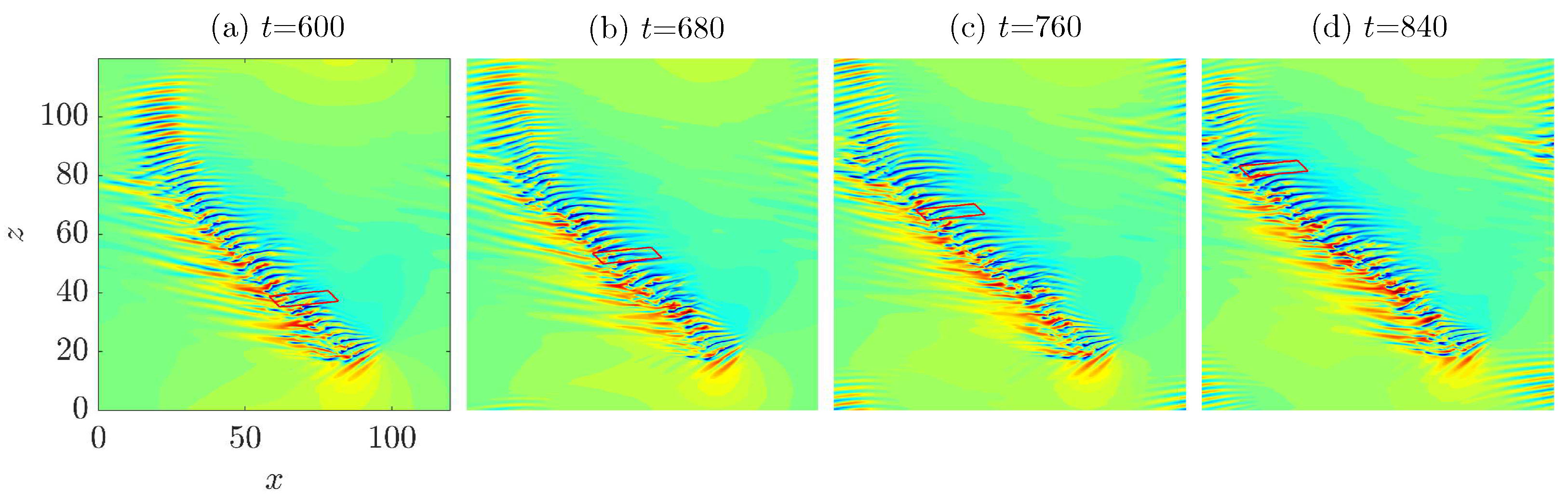
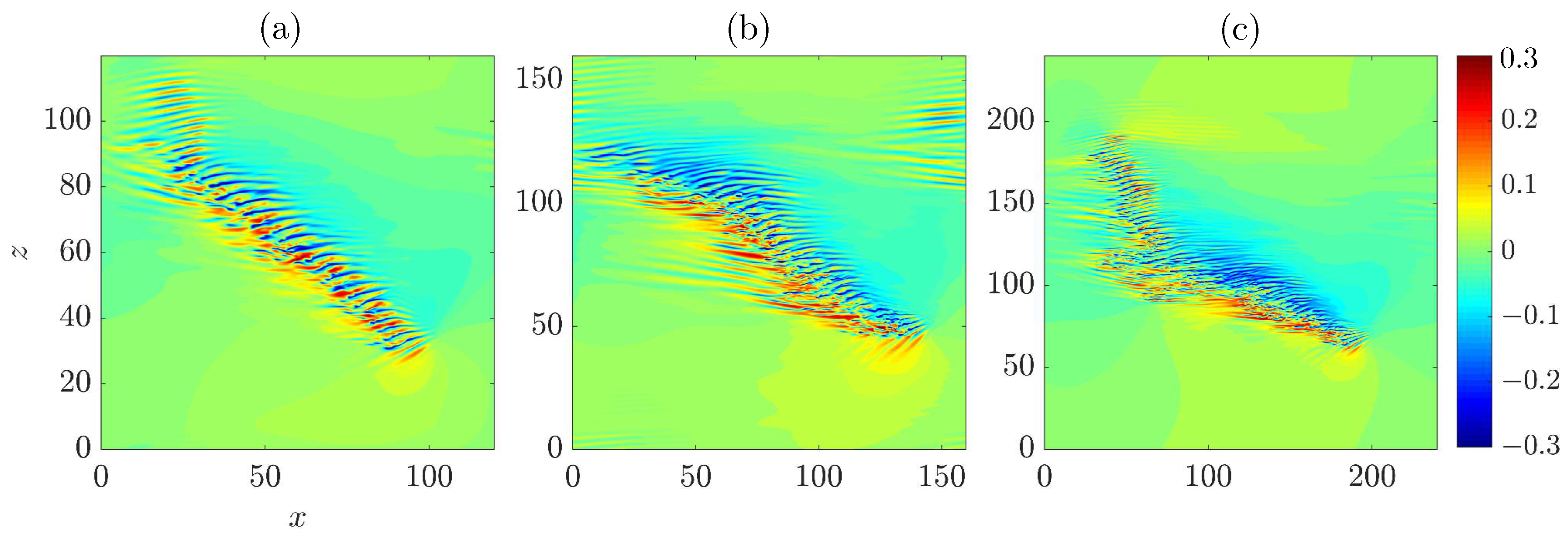
The possible reason for the significant difference between our calculation and the experimental measurements at
can possibly be understood by inspecting the structure of the band as
increases (see
Figure 9). We can see that, at
, the band has a well-defined banded structure, i.e., the width (e.g., the streamwise extension) of the band does not significantly change along the band (see
Figure 9a). At
, the tail of the band seems to broaden and the width of the band may not be constant along the length direction any more (see
Figure 9b). Further at
, the band significantly delocalizes: The bulk broadens gradually towards the tail and part of the band turns into an extended turbulent area (see
Figure 9c). By image processing the entire band, as in the measurements of Paranjape [
9] and Tao et al. [
6], the calculated tilt angle at
will certainly be smaller than our calculation that is only based on the information of the low-speed streaks and the head. This disagreement will be small at low Reynolds numbers when turbulence is well-banded.
The agreement between our calculation and the reported speeds in the literature supports our speculation that the tilt angle of the band is determined jointly by the propagation speed of the head and the advection speed of the streaks inside the bulk. However, what mechanism determines the advection speed of the streaks is still to be investigated. A quantitative study of the large-scale flow may give a hint to the advection of the streaks [
9,
27,
29,
30].
It should be noted that the two ends of turbulent bands may not exist in relatively small normal periodic domains or narrow tilted domains, therefore, seemingly our formulation of the tilt angle (Equation (
1)) does not apply. In those cases, it is not clear what mechanism determines the tilt angle of turbulent bands. Our speculation is that the tilt angle may be indefinite and is strongly affected by the specific domain selection if the head does not exist. This might explain, for the same Reynolds number, why turbulent bands can exist in tilted domains with very different tilt angles [
4,
9,
20] and why the nonlinear traveling wave solutions that Paranjape et al. [
19] obtained can exist in a broad tilt-angle range from
to
.
5. Discussion
The wave generation at the head, the tilt direction, the advection of the head, the streaks inside turbulent bands and the tilt angle of the band are discussed and investigated in this paper. The inflectional-instability argument of Xiao and Song [
24] for the wave generation at the head and its potential relationship with the localized periodic-orbit theory of Kanazawa [
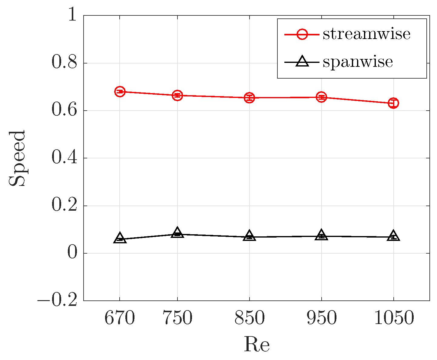
7] are discussed. Based on the discussion, we propose that the tilt direction should probably be determined by the local inflectional spanwise velocity profile generated/introduced by the initial perturbation. The opposite tilt directions are rooted in the mirror symmetry of the spanwise velocity component. Besides, we measured the propagation speed of the head and the advection speed of the low-speed streaks in the bulk of turbulent bands at low Reynolds numbers up to
. We found that the head propagates at constant speeds of
and
(absolute value) at all Reynolds numbers investigated. The low-speed streaks are advected roughly at the speed of the bulk speed in the streamwise direction with a slight decreasing trend as the Reynolds number increases, and the spanwise advection speed is nearly constant at approximately 0.07. Prior studies measured the tilt angle by treating the band as a tilted object [
6,
9]; alternatively, we here propose that the tilt angle of turbulent bands should be determined by the kinematics of the head and the streaks generated at the head. Specifically, the tilt angle can be calculated using the relative speed between the streaks in the bulk and the head, and, at least for
, we obtained a good agreement with the experimental measurements of Paranjape [
9]. We also speculate that the tilt angle of a band may be indefinite and system-dependent if the head does not exist as in narrow tilted domains and relatively small normal domains.
A few problems remain poorly understood and should be investigated in order to further understand the transition in channel flow.
The sustaining mechanism of the wave-generating head. The formation and sustainment of the locally inflectional flow at the head, whether or not the head is locally self-sustained and the relationship between the head and the large-scale flow are still not clear. If the head is indeed locally self-sustained and independent of the bulk, as proposed by Kanazawa [
7], how the flow can be locally excited to this periodic orbit is also not clear. This problem is relevant to the generation and control of turbulent bands at low Reynolds numbers.
The mechanism underlying the advection speed of the head. Xiao and Song [
24] speculated that the speeds are possibly determined by the speeds of the unstable waves resulting from the local inflectional instability. They reported a close spanwise speed of the most unstable wave for
, which is about
and is close to the actual spanwise of the head (see
Figure 2). However, the streamwise speed of the most unstable wave is roughly 0.55 (can be calculated from the eigenvalues and wavenumbers associated with the most unstable wave reported by them) and is significantly lower than the values shown in
Figure 2, which is about 0.85. This discrepancy may be attributed to the over-simplification of the local mean flow at the head by temporal and spatial averaging in their linear stability analysis, as well as by the region selection for the averaging. A possibility to elucidate the mechanism underlying the advection speed is to investigate the speed of the periodic orbit of Kanazawa [
7].
The mechanism underlying the self-sustainment and advection speed of the streaks. Paranjape et al. [
19] obtained exact traveling wave solutions that have some key characteristics of turbulent bands and identified the solutions as the precursors of turbulent bands. Further, for these solutions, they speculated that the streaks are sustained by the tilting effect of the large-scale flow, instead of the self-sustaining process of wall turbulence at high Reynolds numbers in which sinuous streaks break down, generating streamwise vortices, and are regenerated by streamwise vortices [
31,
32]. The same mechanism may also apply to turbulent bands. In our simulations, we indeed observed that streaks in the bulk are long-lived and move with a characteristic speed without a clear breakdown and regeneration. Duguet and Schlatter [
27] described turbulent bands in plane shear flows as the advection of small-scale structures (streaks and vortices) by the large-scale flow, which also seems to suggest the important role of the advection by the large-scale flow in the sustainment of the streaks.
The mechanism underlying the decay of streaks at the tail as well as the splitting and branching of turbulent bands. At relatively higher Reynolds numbers, a band may also nucleate a band with the opposite tilt direction [
8,
9]. The splitting scenario, at least partially, determines the flow pattern.
6. Materials and Methods
For solving the incompressible Navier–Stokes equations in channel geometry, we used our in-house code as described in [
24,
25], which adopts a high-order finite-difference method with a centered nine-point stencil in the wall-normal direction and Fourier-spectral method in the periodic streamwise and spanwise directions. Readers are referred to
Openpipeflow [
33] for details about the finite-difference scheme and the parallelization of the code. The Navier–Stokes equations were integrated using the method of Hugues and Randriamampianina [
34], which adopts a second-order-accurate backward-differentiation scheme, combined with the Adamas–Bashforth scheme for the nonlinear term, for the temporal discretization and a projection method to impose the incompressibility condition. The time-step size was fixed at
for the simulations presented in this paper, which was shown to be sufficiently small for the Reynolds number regime considered [
4,
6].
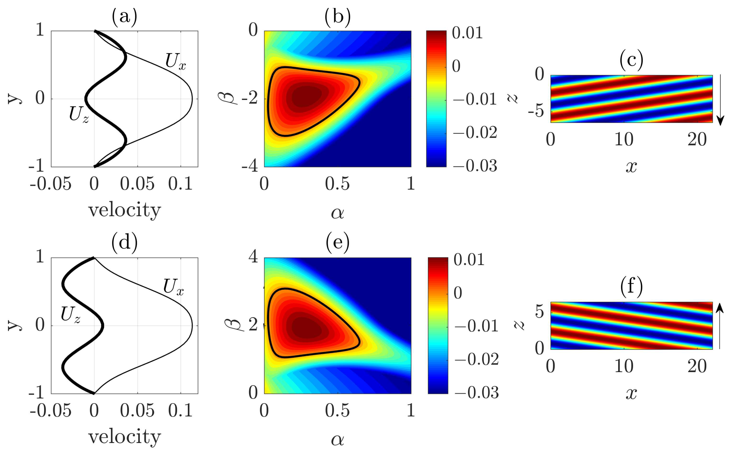
We adopted the method proposed by Song and Xiao [
25] to generate turbulent bands in large domains. The method firstly derives a body force that is needed to maintain an inflectional velocity profile that bears a sufficiently strong instability. Given a target velocity profile
, the body force is derived as
Then, the body force is multiplied by a localization factor such that the force is localized in the
x-
z plane. The size of the localization region should be comparable with the size of the head of a turbulent band and the forcing region is moved at the speed of
(absolute value) and
(see
Figure 2). If the profile
is sufficiently inflectional, the instability can generate sufficiently strong tilted waves (streaks and vortices) and trigger turbulent bands. Once triggered, the length of the band increases, and the force can be switched off after the band has sufficiently developed. The tilt direction of the band can be controlled by the signs of the spanwise component of
and the moving speed
.
We measured the advection speed of the low-speed streaks inside the bulk using the Structural Similarity Index Measure (SSIM) method proposed by Wang et al. [
28], which is commonly used in image processing to measure the similarity between two images. The SSIM index is defined as:
where
x and
y are one-dimensional vectors containing all the pixel values of the two images to be compared, respectively, and
and
measure the luminance, contrast and structural similarity, respectively. The exponents
,
and
are used to tune the relative weight of respective factor, and here we set all of them to 1 according to the suggestion of Wang et al. [
28]. In Equation (
4),
and
denote the mean of
x and
y, respectively. In Equation (
5),
and
denote the standard deviation of
x and
y, respectively. In Equation (
6),
is the covariance of
x and
y. Parameters
and
, where
and
are set to 0.01 and 0.03, respectively, and
L is the maximum of the pixel value, which is set to 255 for unit8 data and 1 for floating point data. In our calculation, the flow velocities, which are floating point data, were taken as the pixel value
x and
y. The parameter
is set such that
in practice according to the suggestion of Wang et al. [
28]. Thus, we have
The result is a value between −1 and 1, and the larger is the result, the higher is the similarity.
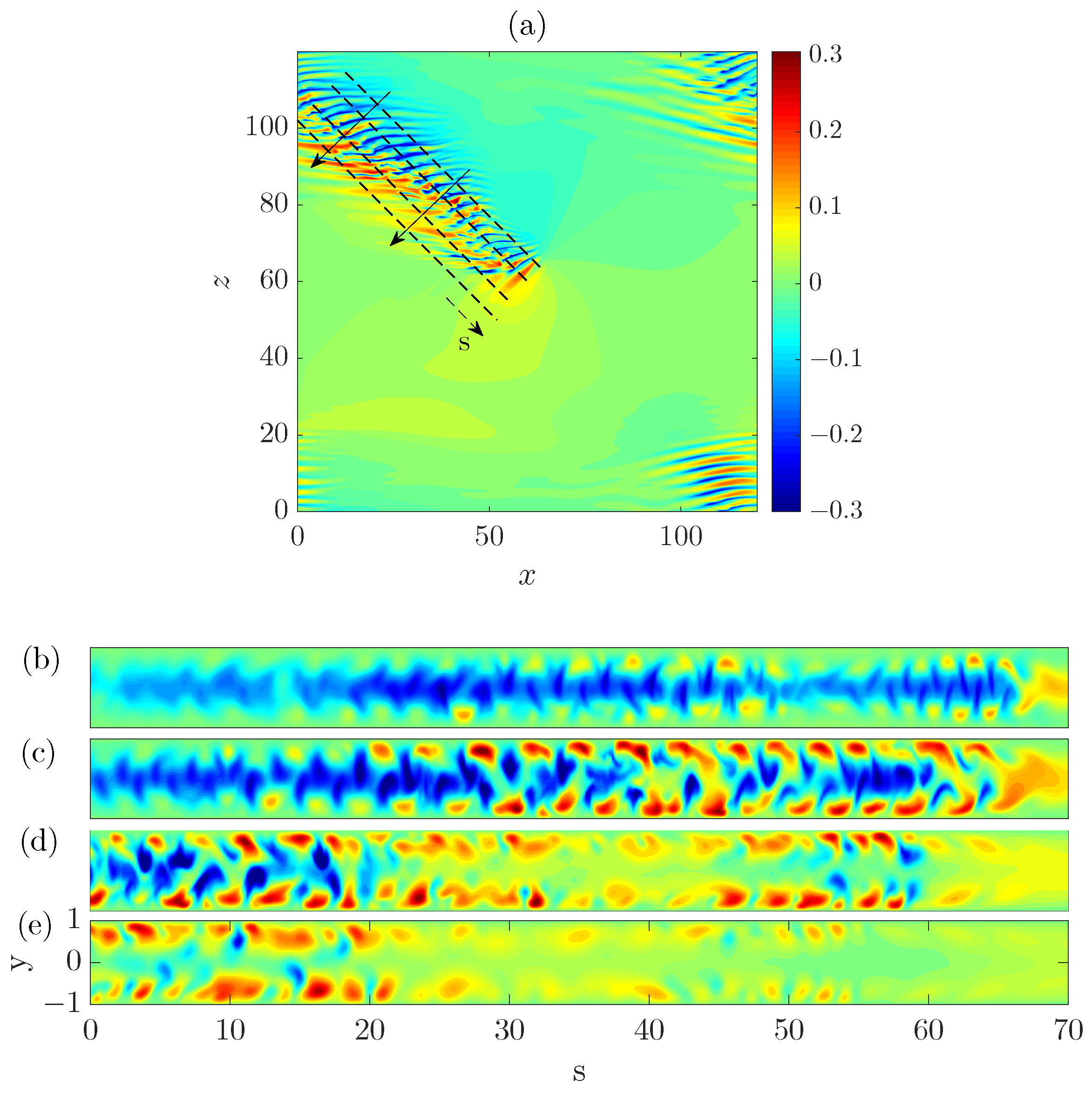
Firstly, we take the streamwise velocities in the cut plane
from two different snapshots
and
that are separated in time by
, after the tilt angle of the band has stopped changing considerably due to the initial transients. In the frame of reference co-moving with the head, i.e., moving with a streamwise speed of 0.85 and a spanwise speed of
(we considered a right-going band), the bulk of the band is located in a nearly fixed area (see
Figure 10). Therefore, we set a rectangular area in which the data inside were considered for calculating the SSIM index. We set the data outside this area to zero so that we eliminated the influence of the data outside this area. Further, to highlight the low-speed streaks, only the streamwise velocities in this area that satisfies
and
were retained. Secondly, we shifted the data from
inside the rectangular over the time separation
with a streamwise speed
and a spanwise speed
. The original data from
and the shifted data from
were used to calculate the SSIM index. Thus, for a given speed pair
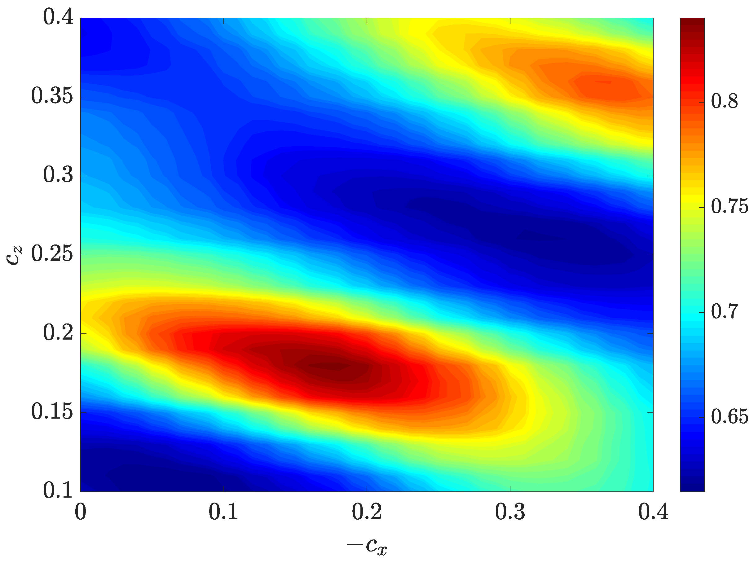
, there is a corresponding SSIM index. By varying the speed pair, the SSIM index will maximize with certain speeds, which we considered as the mean advection speeds of the streaks. The contours of the SSIM index in the
and
for
are shown in
Figure 11.
Note that, in practice, we set
and
to be between 0.1 and 0.4 (the band we considered is a right-going one; therefore,
and
) because the actual speeds were estimated by eye to exist in this range, and note that the shift speeds are relative to the propagation of the head. Obtaining the contours of the SSIM index, we could estimate the advection speed of the streaks to be
and
, i.e., the location of the local peak at the left-bottom corner in
Figure 11. It can be seen that there is another local peak at the right-top corner, which shows a lower SSIM index. That peak was reached when the
data were shifted by more than one wave-length associated with the pattern of the low-speed streaks. The lower SSIM index of the top-right peak, i.e., lower similarity, indicates that the streaky pattern slowly change as it is advected in the bulk.
Note that the time separation
between
and
cannot be too small, otherwise the streaks would have moved too little over the time separation and the speed measurement would be inaccurate. Likewise, it cannot be too large in which case the streaks would have moved by multiple wavelengths, which would also affect the speed calculation. In practice, estimated by eyes, a value between
and 15 is a good choice, and
in
Figure 10 and
Figure 11. In the end, by varying the time instant of
, we can obtain the average advection speed as a function of time and calculate the temporal average, which is plotted in
Figure 7 (the speed of the head is added back in that figure).


