Determining the Bulk Parameters of Plasma Electrons from Pitch-Angle Distribution Measurements

1. Introduction

The environment of interplanetary space is filled with a very low-density plasma, primarily consisting of electrons and protons with a small component of heavier ions. Typically, investigations of this plasma measure the flux of particles in energy and angle to determine the velocity distribution function (VDF) of different particle species. The VDF indicates how energy is distributed between particles of the same type, and can be analysed accordingly to provide bulk properties of the plasma such as density, velocity, and temperature. The accuracy of the derived plasma bulk parameters depends on the accuracy of the measurements and on the techniques we use to analyse the data.

The velocities of space plasma particles often follow kappa distribution functions (see, e.g., in [1,2,3,4,5,6] and references therein). The kappa index labels and governs these distributions and it is another fundamental parameter that describes the thermodynamic state of the plasma. Theoretical works derived the kappa distribution from the foundations of Tsalis non-extensive statistical mechanics (see, e.g., in [7,8,9]). In addition, a large number of studies have determined kappa distribution functions in space plasma environments, such as the solar wind (see, e.g., in [10,11,12,13,14,15]), planetary magnetospheres (see, e.g., in [16,17,18]), cometary electrons (see, e.g., in [19]), and the outer heliosphere and inner heliosheath (see, e.g., in [20,21,22,23,24,25,26]).

The high energy “tails” that characterize kappa distributions are associated with relatively low particle fluxes, and are thus not always clearly resolved in plasma measurements. In these cases, the analysis becomes challenging, because a smaller number of particles are measured leading to a higher statistical uncertainty. Nevertheless, the accurate description of the plasma requires the determination of the kappa index [2,3,27]. Therefore, it is essential to obtain high-quality measurements that resolve the high-energy tails of the plasma distribution functions, and to use the appropriate analysis methods to determine the plasma bulk parameters from the observations.

Typical electrostatic analysers measure the flux of plasma particles over a finite range of energy and flow direction, at a given time. An almost complete scan through energies and directions is achieved by changing the voltages of the instrument components in a consecutive order. Space plasma is permeated by magnetic field which provides an important direction for anisotropy in the plasma. Charged particles gyrate around the magnetic field and particles can move relative to the magnetic field due to drift motions. The magnetic field is also an important direction for the propagation of plasma waves, wave-particle interactions, damping, heating and the generation of waves via instabilities from free-energy in the particle VDFs. Thus, in some operation modes, the measurement cycle of a plasma instrument is modified, and the instrument samples the particle energies in a limited range of directions only, providing the measurements to construct the two-dimensional (2D) pitch-angle distribution function of the plasma. Although the reduction by one dimension allows faster scans which provide high time-resolution measurements, it reduces the statistical significance of the data because the distribution is resolved in fewer points in velocity space.

For example, the Plasma Electron and Current Experiment (PEACE) instrument [28] on board Cluster is designed to measure the plasma electrons within the Earth’s magnetosphere. PEACE consists of two top-hat electrostatic analysers, with look directions onto a plane perpendicular to the spin axis of the spacecraft. During the nominal operation mode, PEACE constructs the three dimensional (3D) VDF of the plasma electrons over the energy range from 0.59 eV to 26.4 keV. The 3D VDF can be constructed over half a spin period of the spacecraft, which corresponds to 2 seconds. In cases when the magnetic field direction lies within the instrument’s azimuthal field of view, we can construct the pitch angle distribution of the plasma electrons over a time period of just 62.5 milliseconds—the time it takes for the instrument to scan in energy.

As another example, the Solar Wind Analyser’s Electron Analyser System (SWA-EAS [29]) on board Solar Orbiter, will measure the solar wind electrons in the energy range from 1 eV to 5 keV, within heliocentric distances from ~0.3 to 1 au. In its nominal operation mode, SWA-EAS completes an energy-direction scan constructing the entire 3D VDFs of the plasma electrons in ~1 s. In burst-mode, the instrument will measure the 2D pitch-angle distribution of the electrons over a period of 0.125 s, using a single deflection state. The accuracy of the derived plasma bulk parameters is a function of the electron flux, which depends on the solar wind density, and speed. Since Solar Orbiter will observe plasma within a wide range of heliocentric distances and heliographic latitudes, we expect a wide range of plasma fluxes to be sampled.

In this study, we investigate the accuracy of our derivation of the plasma bulk parameters, such as the plasma density, temperature tensor and kappa index, from the analysis of the expected 2D pitch-angle measurements by SWA-EAS on board Solar Orbiter. We model the expected measurements of solar wind plasma electrons, considering the instrument’s ideal response, based on the initial instrument calibration. We then fit the synthetic dataset with an analytical model in order to derive the bulk parameters of the electrons. We compare the derived parameters with those from our input. Through this comparison, we quantify the accuracy of the derived parameters as a function of the recorded counts. In Section 2, we describe in detail our instrument model and how we model and analyse the expected observations. In Section 3, we present our results, which we discuss in detail in Section 4. Section 5 summarises our conclusions.

2. Methods

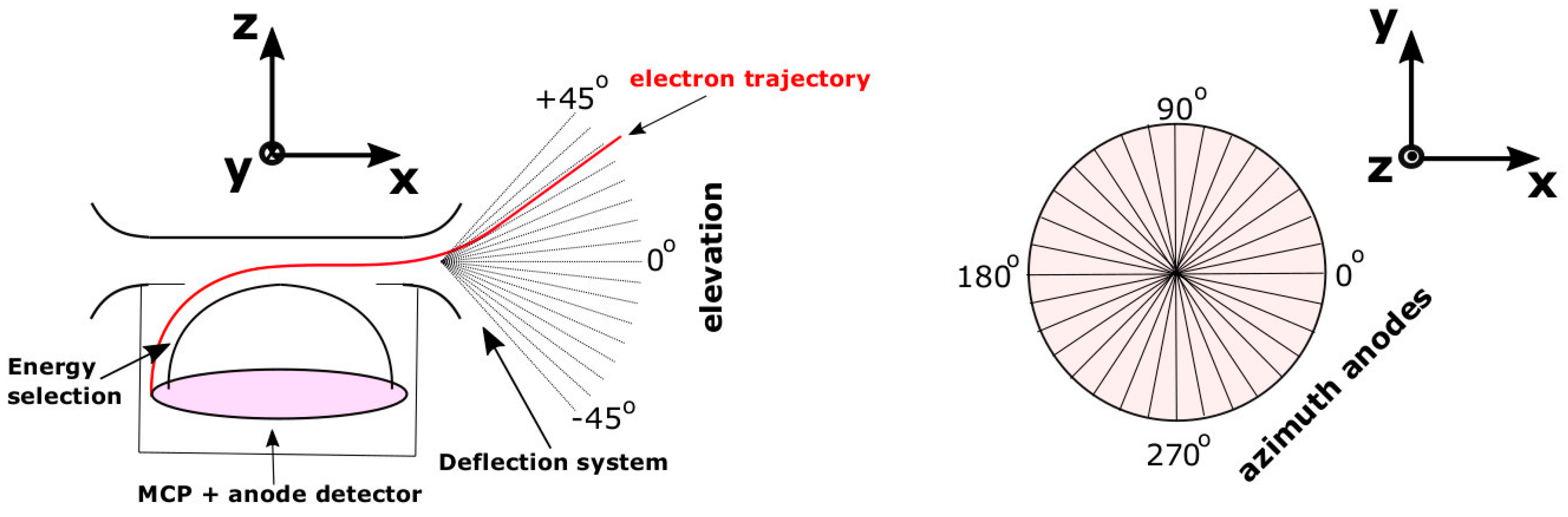
2.1. Instrument Model

SWA-EAS consists of a pair of top-hat electrostatic analyser heads, orthogonally mounted on the spacecraft boom. Each analyser head includes an aperture deflector system and a position-sensitive multichannel plate (MCP) detector. The instrument measures the plasma electron fluxes as a function of kinetic energy and angle of incidence from which the electron VDF is calculated. SWA-EAS scans the energy of the electrons by electrostatic selection in 64 steps, spread exponentially over the range between 1 eV to 5 keV. Each specific kinetic energy step E has a width of ΔΕ/Ε ~ 12.5%. In the nominal operation mode, the aperture deflector system of each analyser head uses voltages applied to plates at the aperture entrance to deflect incoming electrons and scans through the elevation direction of the plasma particles, defined as the complement of the angle within the particle velocity vector and the z-axis perpendicular to the top-hat aperture plane (left panel of Figure 1). Each of the two SWA-EAS analyser heads measure specific elevation directions Θ within the range from −45° to +45° in 16 uniformly spaced electrostatic steps. We model an ideal response in which each Θ is measured with a resolution of ΔΘ = 6°. The azimuth direction is the angle within the projection of the velocity vector on the top-hat plane (x-y plane) and the x-axis (right panel of Figure 1). Each SWA-EAS analyser head resolves 32 discrete azimuth directions Φ covering the full range from 0° to 360° by 32 azimuth sectors mounted on the MCP. Each azimuth direction Φ has a resolution of ΔΦ = 11.25°. Combining two of the analyser units offset by 90° allows the full sky to be measured. Thus, one analyser can always see the direction towards the magnetic field vector $\overrightarrow{B}$. In burst-mode operations, the analyser head that can see $\overrightarrow{B}$ performs two consecutive energy scans; one with the aperture deflectors set to Θ = θ_B, followed by a scan with the deflectors set to Θ = −θ_B, where θ_B is the elevation angle of the magnetic field vector, which has been recorded by the magnetometer on board Solar Orbiter [30] just before the EAS scan. Thus, the flux of electrons will be measured in two cones, one with an edge aligned along and one anti-parallel with $\overrightarrow{B}$. From these measurements a pitch-angle distribution can be recovered.

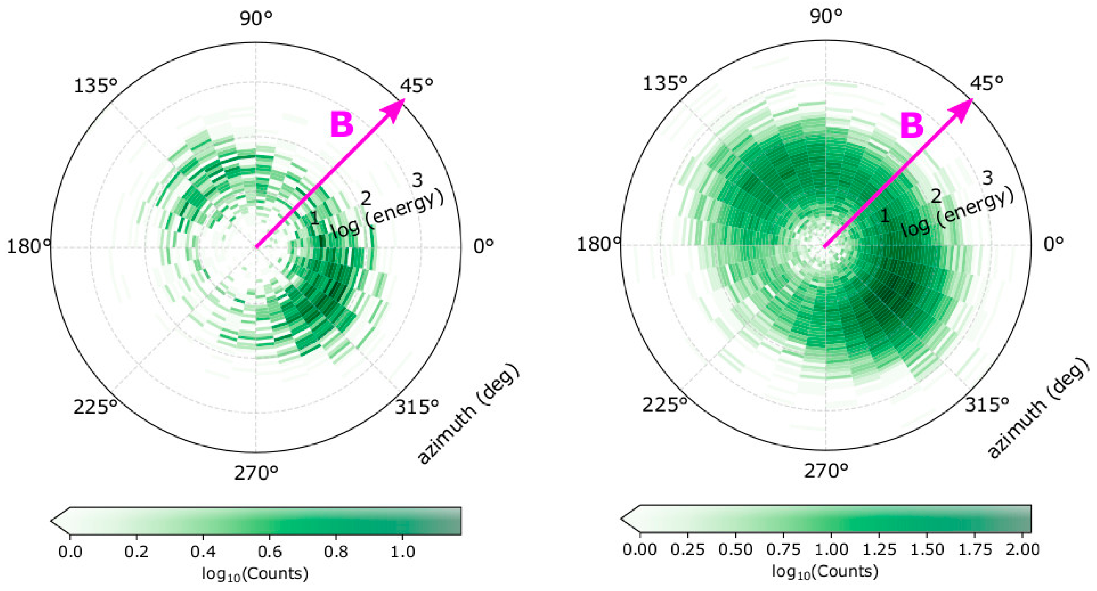
2.2. Synthetic Dataset

We use the well-established forward-modelling technique (see, e.g., in [31,32,33,34,35,36,37,38,39]) to simulate the expected SWA-EAS observations in the solar wind. We focus on the characterization of supra-thermal electrons, which we consider more challenging due to the high energy tails of their VDFs. We model solar wind electrons with their velocities following the bi-kappa distribution function (see, e.g., in [3,4,5,6])

$$f(\overrightarrow{u})=\frac{n}{\sqrt{T_{\parallel }}{T}_{\perp }}{\left[\frac{{\mathrm{m}}_{\mathrm{e}}}{2\mathsf{\pi }\left(\kappa -3/2\right){\mathrm{k}}_{\mathrm{B}}}\right]}^{3/2}\frac{\mathsf{\Gamma }(\kappa +1)}{\mathsf{\Gamma }(\kappa -1/2)}{\left[1+\frac{{\mathrm{m}}_{\mathrm{e}}{(u_{\parallel }-u_{0,\parallel })}^2}{2{\mathrm{k}}_{\mathrm{B}}\left(\kappa -3/2\right)T_{\parallel }}+\frac{{\mathrm{m}}_{\mathrm{e}}{({\overrightarrow{u}}_{\perp }-{\overrightarrow{u}}_{0,\perp })}^2}{2{\mathrm{k}}_{\mathrm{B}}(\kappa -3/2)T_{\perp }}\right]}^{-\kappa -1},$$

(1)

where n is the electron number density, $u_{\parallel }$, ${\overrightarrow{u}}_{\perp }$ are the particle velocity parallel and perpendicular to the magnetic field respectively and $u_{0,\parallel }$ and ${\overrightarrow{u}}_{0,\perp }$ are the corresponding bulk velocities. $T_{\parallel }$, and $T_{\perp }$ are the parallel and the perpendicular temperature, respectively, and κ is the kappa index. Finally, Γ is the gamma function, k_B is the Boltzmann constant and m_e is the electron mass.

We consider a simple set-up with $\overrightarrow{B}$ in the top-hat plane of an individual SWA-EAS analyser head (magnetic field elevation angle θ_B = 0°) and the analyser head performing a single scan through kinetic energy E and azimuth Φ, for elevation Θ = θ_B = 0°, with acquisition time Δτ. The instrument records an expected number of counts,

$$C_{\exp }(E,\Theta ={\theta }_{\mathrm{B}}=0,\Phi )=\frac{2}{{\mathrm{m}}_{\mathrm{e}}{}^2}Gf(E,\Theta ={\theta }_{\mathrm{B}},\Phi )E^2\Delta \tau ,$$

(2)

where

$$G=A_{\mathrm{eff}}\frac{\Delta E}{E}\Delta \Theta \Delta \Phi ,$$

(3)

is the geometric factor of the instrument and A_eff is the effective area, which is a function of the instrument’s aperture and the detector’s efficiency. For this study, we assume a constant A_eff which results in a constant G, although in reality, both could be functions of energy, elevation and azimuth. For further simplification, we only consider cases in which the bulk velocity vector points towards the x-axis, so that the elevation and the azimuth angle of the bulk velocity vector θ_u,0 = φ_u,0 = 0°. We also set the azimuth angle of the magnetic field to φ_B = 45°. We note that in this specific set-up, the bulk speed components have the same magnitude $\left|{\overrightarrow{u}}_{0,\parallel }\right|=\left|{\overrightarrow{u}}_{0,\perp }\right|$, and the azimuth sectors of the instrument measure the pitch-angles of the particles. We assume that the registered counts C follow the Poisson distribution:

$$P(\mathrm{C})=e^{-C_{\exp }}\frac{C_{\exp }{}^C}{C!}.$$

(4)

In Figure 2, we show two examples of the synthetic datasets, based on electron plasma densities of n = 5 cm⁻³ (left panel), and n = 50 cm⁻³ (right panel). For both examples, the bulk velocity of magnitude u₀ = 500 kms⁻¹ points along the x-axis, and we set κ = 3, $T_{\parallel }$ = 10 eV, and $T_{\perp }$ = 20 eV.

In our approach we neglect effects related to the spacecraft potential. In reality, the spacecraft floats at a potential caused by interaction with the space environment and depending on the composition of materials that cover the surface of the spacecraft. This potential can be of order 10 V or more. Furthermore, UV photons striking the spacecraft produce photoelectrons that form a cloud around the spacecraft. Thus, the incoming solar wind electron population can be accelerated by a few eV and obscured by a high-density population of electrons at all energies below the spacecraft potential. Furthermore, it is possible for the VDF of the electrons to have an irregular shape in 3D. We ignore these effects here as we are interested in the high-energy tail of the electron distribution which should not be affected by these phenomena, and we assume gyrotropy, i.e., that the VDF is symmetrical in rotation around the magnetic field direction.

We derive the plasma properties by fitting our analytical model of the expected counts in Equation (2) to the observations. During the actual operations of SWA-EAS, $\overrightarrow{B}$ will be determined from Solar Orbiter’s magnetometer instrument [30]. Therefore, in our fitting analysis, the parallel and perpendicular directions are known parameters. Moreover, we reduce the unknown parameters of the fitted model by obtaining the plasma bulk velocity vector from proton measurements by the Proton Alpha Sensor (SWA-PAS [29]) on board the same spacecraft. This approach assumes that protons and electrons have the same bulk velocity, which is generally true for plasma with zero net charge and no significant drifts among the ion species. We note, however, that a more sophisticated approach could leave the electron bulk velocity as a free parameter to be derived by the fitting analysis. We then use a chi-squared minimization algorithm which defines the optimal combination of the undetermined plasma parameters (n, κ, $T_{\parallel }$, and $T_{\perp }$) that minimize the chi-squared value

$${\chi }^2=\frac{1}{N-R}{\displaystyle \sum _{i=1}^N{\left[\frac{C_i-C_{\exp ,i}(n^{\prime },{\kappa }^{\prime },T_{\parallel }^{\prime },T_{\perp }^{\prime })}{{\sigma }_i}\right]}^2},$$

(5)

where N is the total number of data-points we consider for fitting, R is the number of the model’s free parameters, and σ_i is the standard deviation of each count C_i. The model we fit to the observations is a function of n, κ, $T_{\parallel }$, and $T_{\perp }$, so R = 4. In plasma applications, we typically use ${\sigma }_i=\sqrt{C_i}$, as within a complete scan, we obtain only one measurement for each specific point in velocity space, and we assume that it represents the average value and the variance of the expected number of particles. For each measurement sample, we perform two fittings; one which excludes all points with C_i = 0, and one which includes all points with C_i = 0 in the analysis. We note that, in the second type of fitting, we assign an uncertainty of σ_i = 1 to each C_i = 0 measurement (see, e.g., in [40]). In Figure 3, we show an example of our synthetic dataset and the corresponding model fitted to it. (The software used in this study is available for download at www.github.com/gnicolaou85/Elfit)

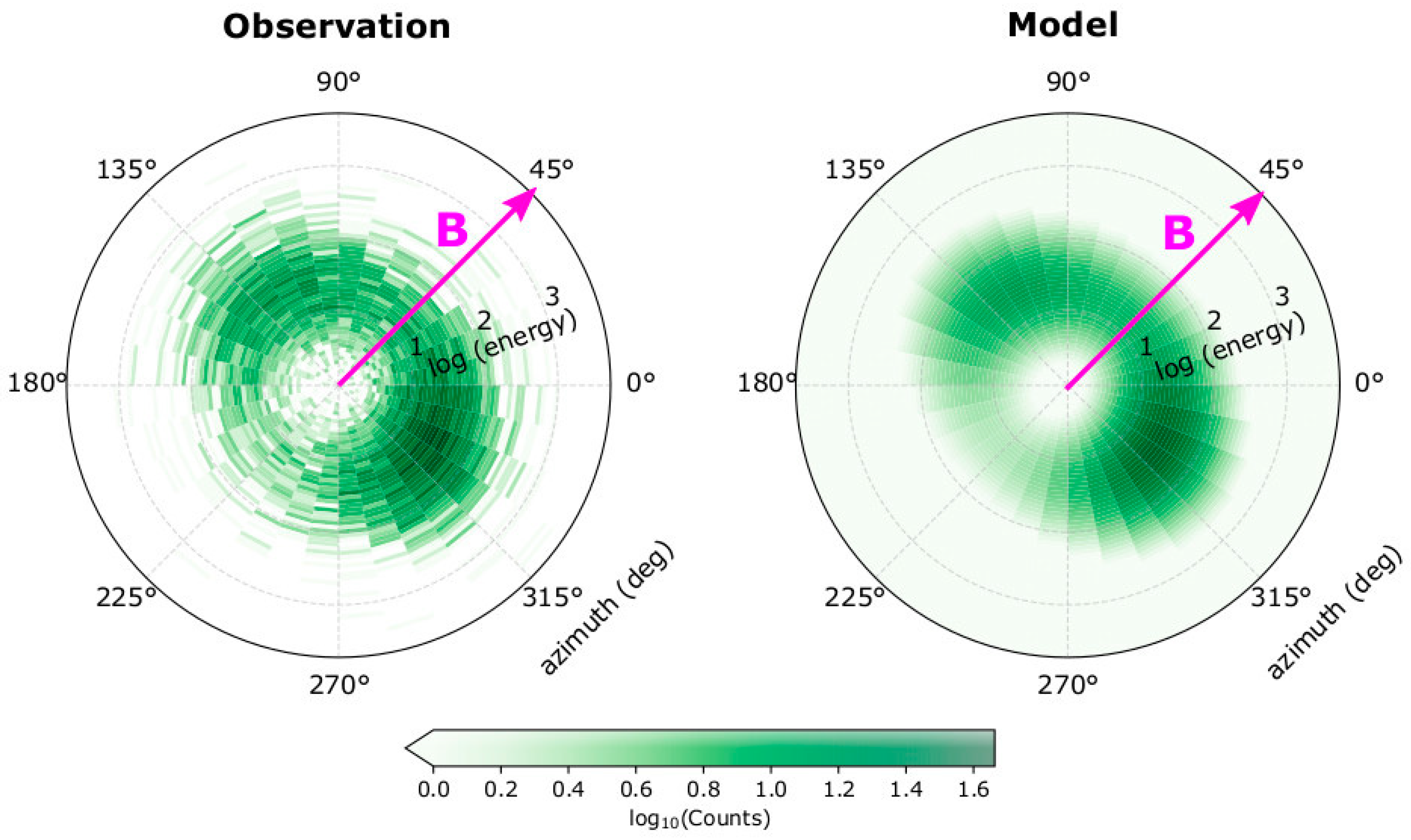
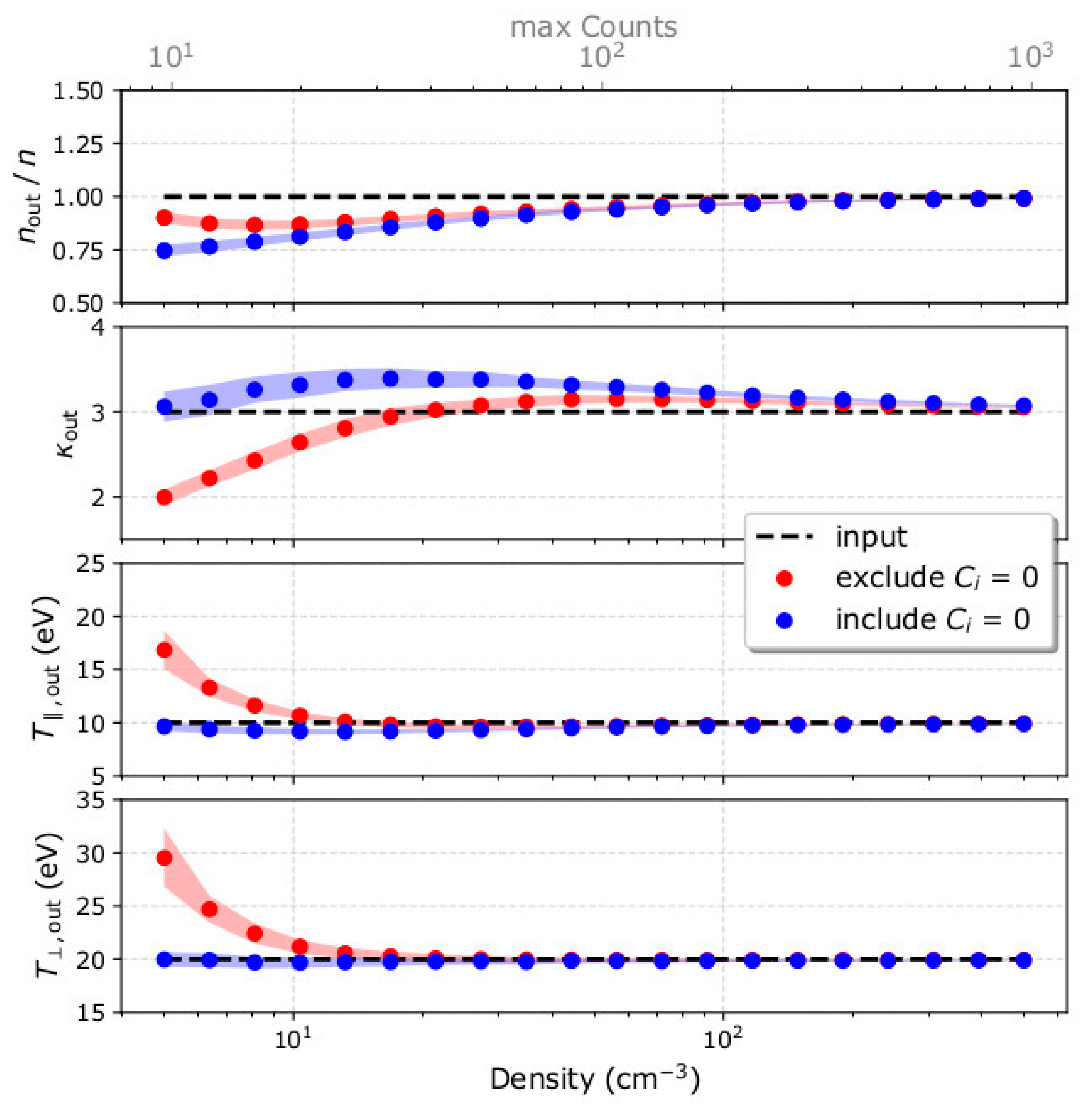
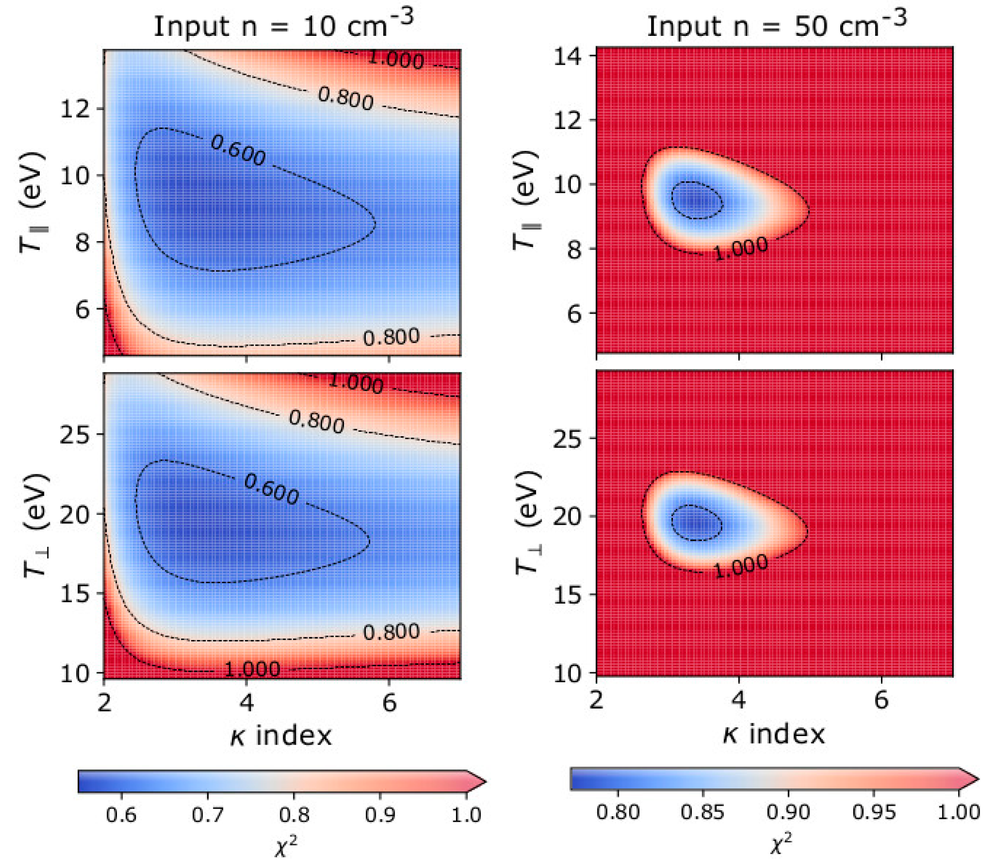
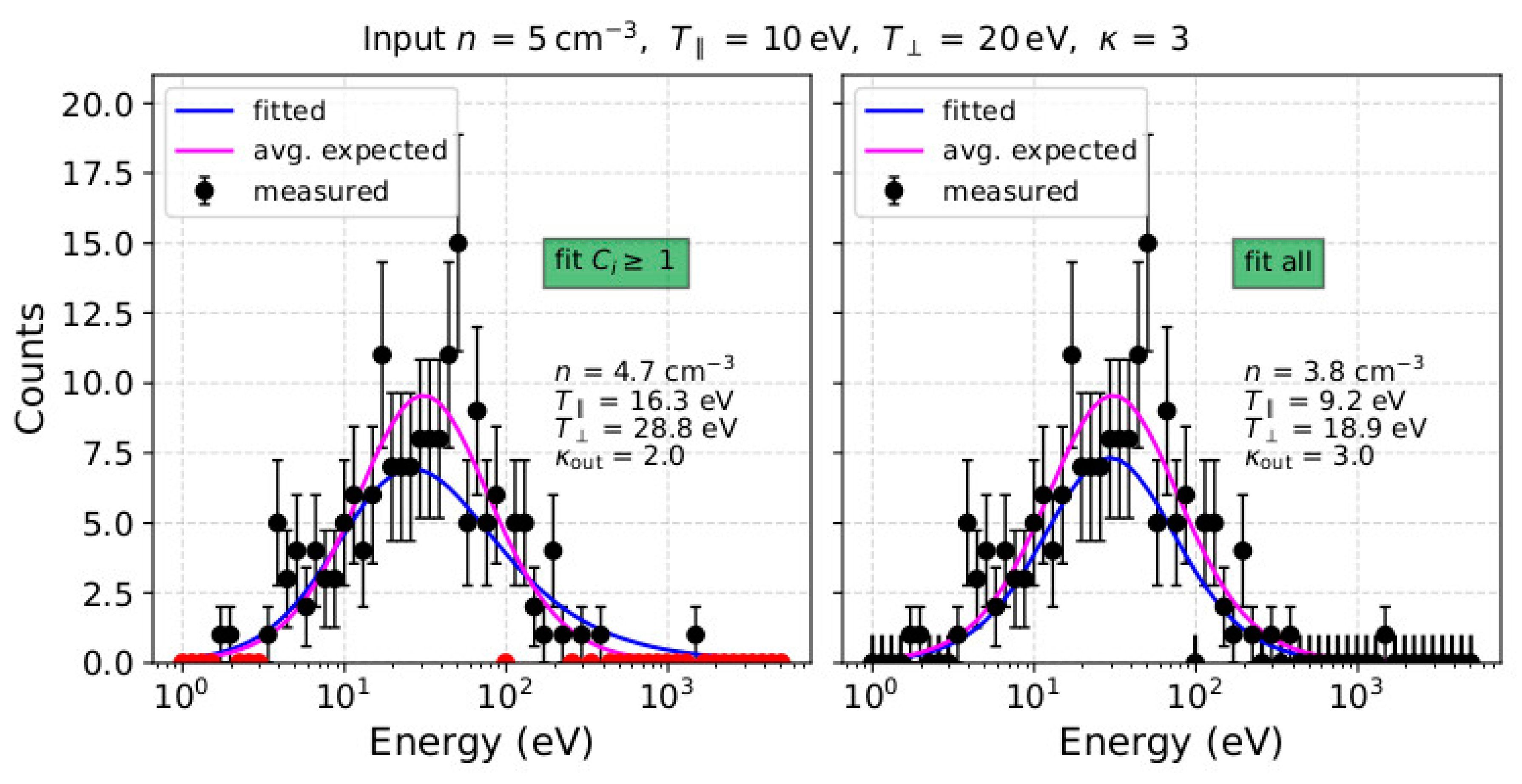
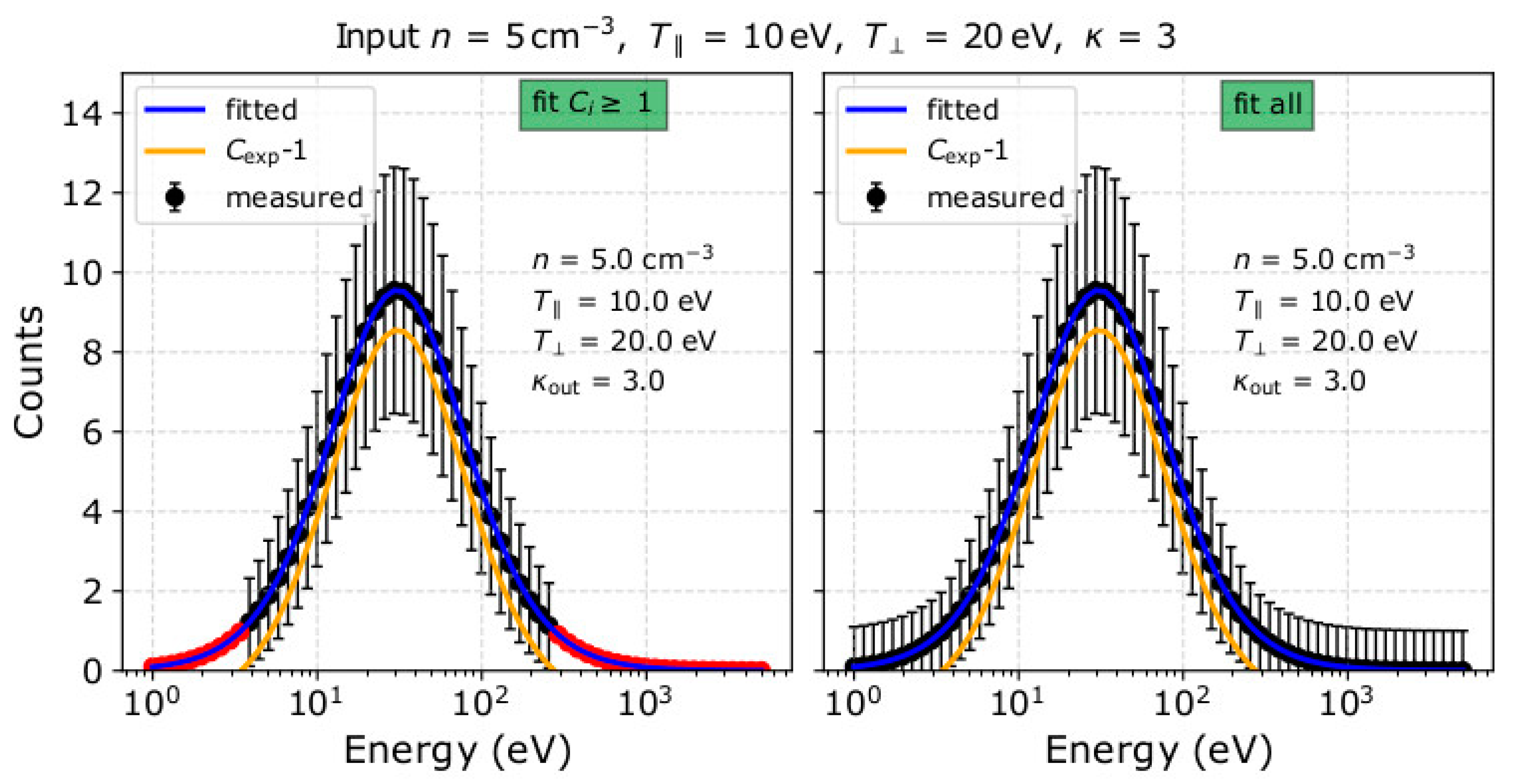
3. Results

For each set of input plasma conditions, we simulate 200 measurement samples which we fit to derive the electron density, temperature and kappa, as explained in Section 2. By investigating the histograms of the derived parameters, we verify that 200 samples are sufficient to derive statistically significant results, especially within the low density (low particle flux) range. The histograms of the derived parameters from the analysis of 200 samples with input parameters n = 7 cm⁻³, u₀ = 500 kms⁻¹ pointing along the x-axis, κ = 3, $T_{\parallel }$ = 10 eV, and $T_{\perp }$ = 20 eV, are shown in Figure 4.

Table 1. The input and the derived bulk parameters for the histograms in Figure 4.

Parameter	Input	Fit Including Ci = 0 Points	Fit Excluding Ci = 0 Points
n (cm−3)	7	5.4 ± 0.2	6.1 ± 0.2
κ	3	3.2 ± 0.2	2.3 ± 0.1
$T_{\parallel }$ (eV)	10	9.4 ± 0.3	12.5 ± 0.7
$T_{\perp }$ (eV)	20	19.8 ± 0.6	23.7 ± 1.0

shows their average values and standard deviations. For these input plasma conditions, the average derived plasma density is by ~23% lower than the input plasma density if the fitting includes C_i = 0, and by ~13% lower than the input density when C_i = 0 are not included in the fit. The standard deviation of the derived densities is ${\sigma }_n$ ~0.2 cm⁻³ for both fits. On average, the fitting analysis that includes C_i = 0 overestimates the kappa index by ~7%, while the fitting that excludes C_i = 0 underestimates kappa by ~23 %. The standard deviations of the derived kappa indices are ~ 0.2 and 0.1 respectively. The average derived $T_{\parallel }$ is by ~6% lower than the actual value when C_i = 0 are included in the fit, and by ~25% larger than the actual value when C_i = 0 are not included in the fit. The standard deviation of $T_{\parallel }$ is 0.3 eV when C_i = 0 are fitted and 0.7 eV when C_i = 0 are not fitted. The fit that includes C_i = 0 derives accurately $T_{\perp }$ within the standard deviation $\sigma T_{\perp }$ = 0.6 eV. The fit that excludes C_i = 0 from the fit overestimates $T_{\perp }$ by ~19%, with standard deviation $\sigma T_{\perp }$ = 1 eV.

The solar orbiter expects densities between ~5 cm⁻³ and ~500 cm⁻³. In Figure 5, we show the derived parameters as functions of the plasma density over the expected range. The red points show the average (over 200 samples) values of the derived parameters as determined by our fits excluding points with C_i = 0, and the blue points show our results for the fit analysis including points with C_i = 0. The shadowed regions represent the standard deviations of the corresponding values. The horizontal axis on the top shows the maximum number of the expected counts (peak value at an individual E, Φ) for the specific input parameters. On the lower side of the density (and counts) range, the plasma density is underestimated in both fitting strategies; however, it is more accurately determined by both fitting strategies when n > 50 cm⁻³ (C_max > 100).

The kappa index is significantly misestimated (up to 35%) over the low input density range, if the analysis excludes points with C_i = 0. For instance, when n = 5 cm⁻³, the derived index κ_out ~ 2. Interestingly, for the same plasma, κ_out is accurately determined when C_i = 0 measurements are included in our fit. However, as the density increases to n > 20 cm⁻³, the kappa index is more accurately determined when derived by fits excluding points with C_i = 0.

For the input parameters we examine, the fitting analysis that excludes points with C_i = 0 significantly overestimates the plasma temperature in the low-density range (n < 10 cm⁻³). For instance, when n = 5 cm⁻³ (C_max ~ 10), the derived $T_{\parallel }$ ~ 17 eV, which is 1.7 times greater than its actual input value, and the derived $T_{\perp }$ ~ 30 eV, which is 1.5 times greater than its actual input value. For the same plasma conditions, when the analysis includes points with C_i = 0, the derived temperatures do not deviate from their actual values by more than 4 %. Nevertheless, the two fitting analyses determine similar temperatures for n > 10 cm⁻³.

Finally, we examine the fit convergence as a function of the plasma parameters; the minimum χ² defines the best fit parameters. Previous studies [27,33] show that the accurate estimation of the plasma temperature depends on the accurate determination of the kappa index. In Figure 6, we show 2D plots of the χ² value as a function of the model parameters κ, $T_{\parallel }$, and $T_{\perp }$. For each panel, we show χ² as a function of two parameters at a time, and we keep the remaining model parameters to their values as determined by the best fit. We perform our calculations for input plasmas with two different densities: n = 10 cm⁻³, and n = 50 cm⁻³. In both examples, we use κ = 3, u₀ = 500 kms⁻¹ pointing along the x-axis, $T_{\parallel }$ = 10 eV, and $T_{\perp }$ = 20 eV as the input parameters. Red areas on the plots in Figure 6 indicate χ² > 1. For a fixed acquisition time Δτ and fixed geometric factor G, higher densities result in higher counts and a smaller area of low χ², which indicates that the derived parameters possess a smaller uncertainty. The non-axisymmetric shape of the area of low χ², indicates an interdependency of the derived kappa index and the temperatures. More specifically, the area of low χ² shifts towards higher temperatures and gets broader along the vertical axis for smaller κ.

4. Discussion

We examine the accuracy of plasma electron bulk parameters as derived from the analysis of the expected observations by SWA-EAS operating in burst-mode. Generally, the accuracy of the derived parameters is a function of the flux of plasma particles (number of recorded counts). Our analysis shows that the fit analysis of samples with a significant amount of counts (C_max > 30), derives accurately the plasma parameters when measurement points with zero counts (C_i = 0) are excluded from the analysis. We show that when analysing observations with a low amount of counts (C_max < 30), the accuracy of some parameters is improved if measurement points with zero counts are included in the fitting analysis.

The uncertainty of each measurement C_i is approximated with ${\sigma }_i=\sqrt{C_i}$, assuming that the recorded signal follows the Poisson distribution. This results to a relative uncertainty $\frac{{\sigma }_i}{C_i}=\frac{1}{{\sqrt{C}}_i}$ which becomes considerably large for small C_i and propagates significant statistical and systematic errors in the derivation of the plasma bulk properties. Although Poisson statistics does not really apply to C_i = 0, these bins indicate points of velocity space with low fluxes which do not reach the detection threshold. This information is still useful, especially when the overall signal is weak.

In Figure 7, we show the distribution of counts as a function of energy, recorded in the azimuth anode which contains the maximum number of counts C_max, assuming a plasma with n = 5 cm⁻³, κ = 3, $T_{\parallel }$ = 10 eV and $T_{\perp }$ = 20 eV. The blue curves in both panels show the analytical model fitted to the data (fitted to the 2D distribution of counts) and the magenta curve indicates the expected number of counts. In the left panel, the fitting analysis excludes measurements with C_i = 0 (red points), whereas in the right panel, the fitting analysis includes measurements with C_i = 0 with standard deviation σ_i = 1. The kappa index of the fitted model in the left panel is ~2, and the distribution’s high-energy tail is prominent up to 2 keV, based on the inclusion of the non-zero data-points beyond ~400 eV, neglecting all points with C_i = 0 in between. On the other hand, the fit result in the right panel does not have a prominent tail extending beyond 400 eV, as it fits all C_i = 0 points within that energy range. In this case, κ_out ~ 3 which is an accurate estimation of the actual kappa index of the modelled plasma.

As we show in Figure 5 and Figure 7, both fitting strategies underestimate the plasma density when the input density is n < 50 cm⁻³. This is partially due to the asymmetry that characterizes the Poisson distributions of low counts. In Figure 8, we show the Poisson distributions for C_exp = 1, C_exp = 3 and C_exp = 5. Each distribution has two modes (most frequent values); the higher mode which is equal to the average value of the distribution C_exp, and the lower mode = C_exp − 1. The relative difference between the two modes increases with decreasing C_exp. Samples drawn from a Poisson distribution with a small C_exp, as is the case at low densities expected to be measured by SWA-EAS at ~1 au, will more likely undersample the distribution than oversample, and so densities will be underestimated. In addition, within a measurement cycle, each point of velocity space is sampled only once. In our analysis, we consider that an individual C_i obtained at a specific point of velocity space is representative of the average value C_exp with uncertainty ${\sigma }_i=\sqrt{C_i}$. This introduces an additional systematic error. We illustrate this error by considering an exemplar Poisson distribution with C_exp = 5. If we obtain one measurement, the probabilities for observing C_i = 1 and C_i = 9 are almost the same (see Figure 8). However, in our fitting analysis, the corresponding uncertainties for C_i = 1 and C_i = 9, are σ_i = 1 and σ_i = 3, respectively, and a χ² minimization model fitted to these two points will shift towards C_i = 1, as the specific point has a bigger weight ${\sigma }_i^{-2}=C_i^{-1}=1$. This specific systematic error purely depends on the statistical uncertainty of the measurements. We prove this by fitting the mean values of the Poisson distribution (or higher mode value) with both fitting strategies (Figure 9). For the specific example, we consider plasma with the same bulk properties as in the example shown in Figure 7 and we show that in the absence of statistical fluctuations, both fits derive identical results. The orange curve in both panels is the lower mode of the Poisson distribution C_exp − 1, which corresponds to a distribution with lower density. In reality, the errors associated with the statistical uncertainty of the measurements decrease with increasing number of counts and/or when analysing average counts over multiple samples of the same plasma.

5. Conclusions

We investigate the accuracy of the electron plasma bulk parameters as derived by our analysis of SWA-EAS high-time resolution measurements. We assume electrons with velocity distribution function following the anisotropic bi-kappa distribution function and simulate the expected counts in the instrument’s frame based on a realistic instrument model. We derive the plasma bulk parameters by fitting the observations with an analytical model, using the χ² minimization method.

Our analysis shows the following.

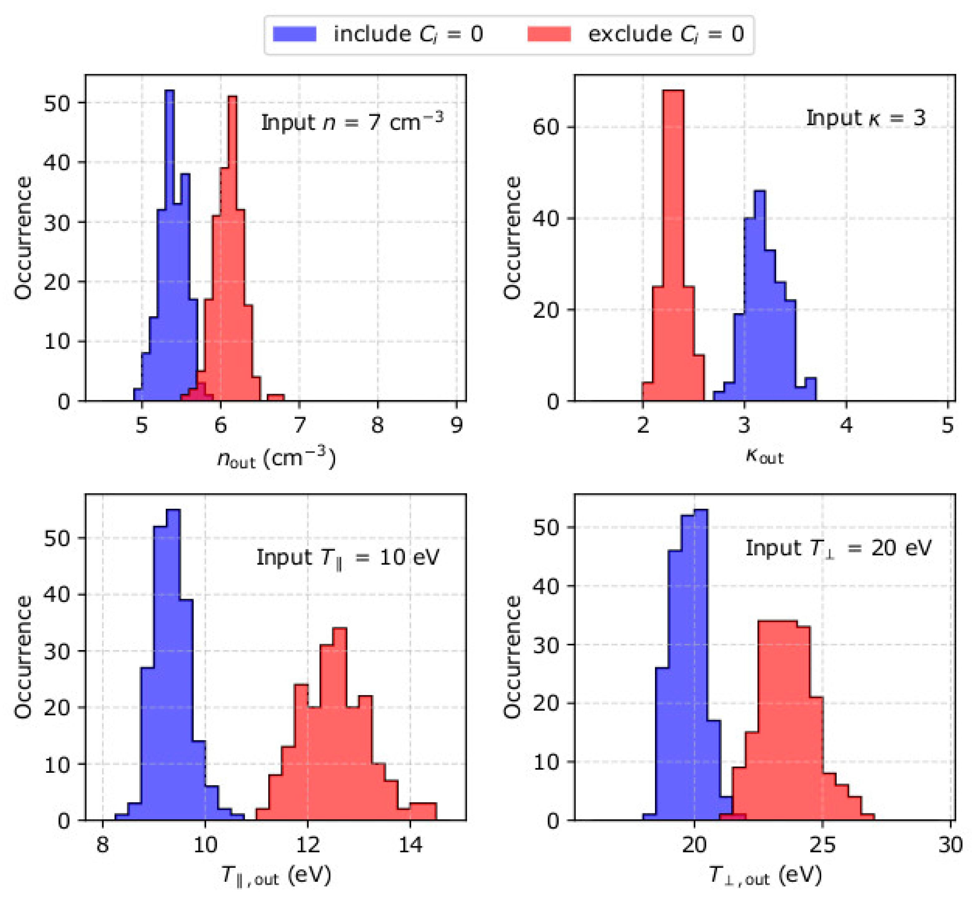
• The fit analysis of plasma measurements with relatively high flux (C_max > 30) estimates the plasma temperature and kappa index more accurately if it excludes measurement points with C_i = 0. The corresponding analysis of measurements with low particle flux (C_max < 30) estimates the temperature and kappa index more accurately if it includes measurement points with C_i = 0. Although C_i = 0 is a measurement with a large uncertainty, it contains information that becomes useful when the overall signal is weak.
• Examination of the fit convergence indicates that the determination of the plasma temperature and the determination of the kappa index are interdependent. As expected, the uncertainty of the derived parameters decreases with increasing particle flux.
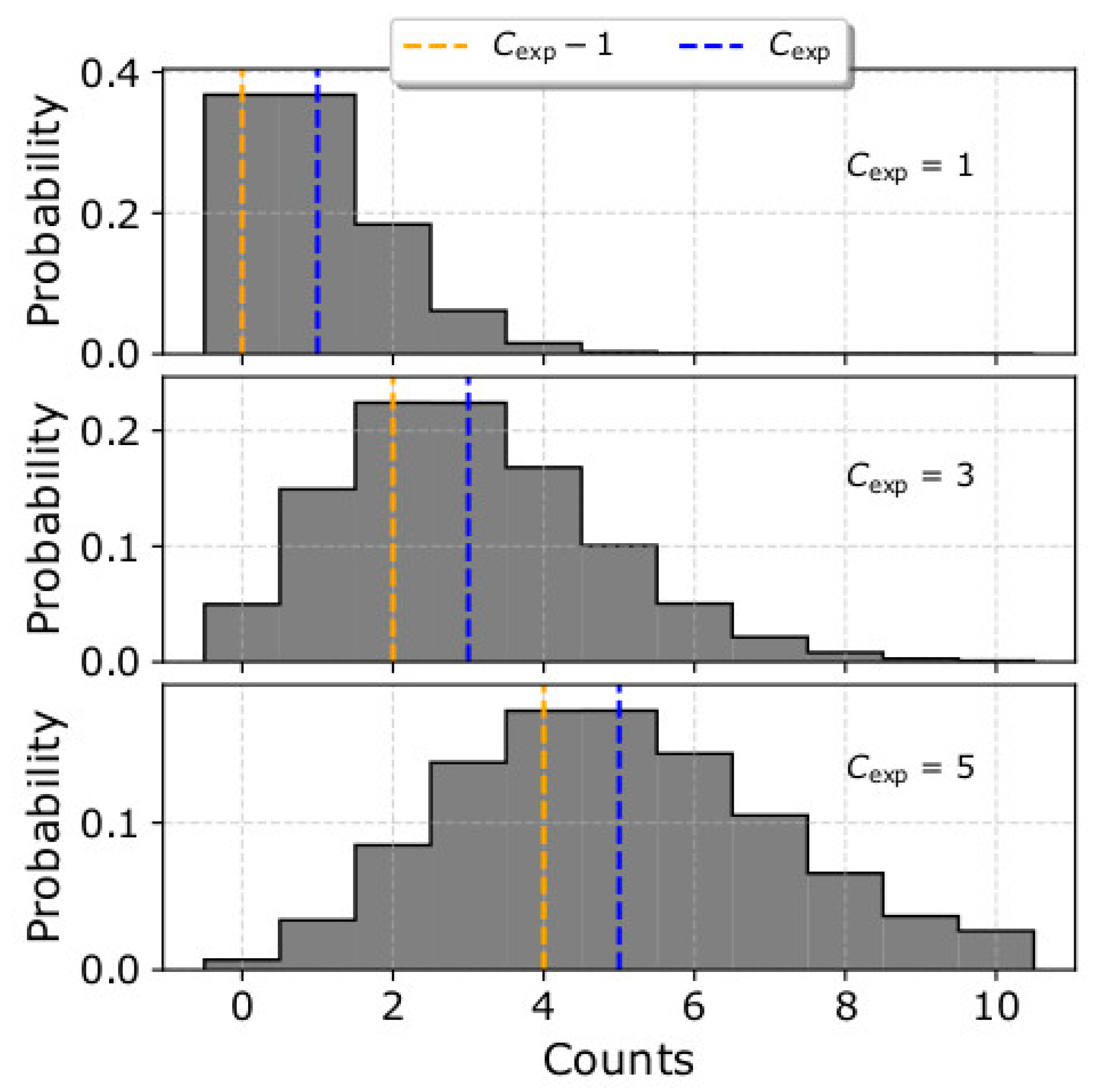
• The plasma density is underestimated when the particle flux is low (C_max < 100). We show that the misestimation is due to the asymmetry of the Poisson distribution and the assigned uncertainties to the data points.

Our study predicts the accuracy of the future SWA-EAS measurements. However, our methods can be applied to investigate and/or improve the accuracy of similar fitting analyses which determine kappa distribution functions. Although this paper uses the kappa distribution to describe the VDFs of plasma particles, the kappa distribution function is used to describe several other mechanisms as well (e.g., the angular scattering of particles passing through graphene and carbon foils [41,42]).

References

- Shizgal, B.D. Suprathermal particle distributions in space physics: Kappa distributions and entropy. Astrophys. Space Sci. 2007, 312, 227–237. [Google Scholar] [CrossRef]
- Livadiotis, G.; McComas, D.J. Beyond kappa distributions: Exploiting Tsalis statistical mechanics in space plasmas. J. Geophys. Res. 2009, 114, A11105. [Google Scholar] [CrossRef]
- Livadiotis, G.; McComas, D.J. Understanding kappa distributions: A toolbox for space science and astrophysics. Space Sci. Rev. 2013, 175, 183–214. [Google Scholar] [CrossRef]
- Pierrard, V.; Lazar, M. Kappa distributions: Theory and applications in space plasmas. Sol. Phys. 2010, 267, 153–174. [Google Scholar] [CrossRef]
- Livadiotis, G. Introduction to special section on origins and properties of kappa distributions: Statistical Background and properties of kappa distributions in space plasmas. J. Geophys. Res. 2015, 120, 1607–1619. [Google Scholar] [CrossRef]
- Livadiotis, G. Kappa Distributions: Theory and Applications in Plasmas; Elsavier: Amsterdam, The Netherlands, 2017. [Google Scholar]
- Tsallis, C. Possible generalization of Boltzmann-Gibbs statistics. J. Stat. Phys. 1988, 52, 479–487. [Google Scholar] [CrossRef]
- Tsallis, C. Introduction to Nonextensive Statistical Mechanics: Approaching a Complex World; Springer: New York, NY, USA, 2009. [Google Scholar]
- Tsallis, C.; Mendes, R.S.; Plastino, A.R. The role of constraints within generalized nonextensive statistics. Physica A 1998, 261, 534–554. [Google Scholar] [CrossRef]
- Maksimovic, M.; Pierrard, V.; Riley, P. Ulysses electron distributions fitted with kappa functions. Geophys. Res. Lett. 1997, 24, 1151–1154. [Google Scholar] [CrossRef]
- Maksimovic, M.; Zouganelis, I.; Chaufray, J.Y.; Issautier, K.; Scime, E.E.; Littleton, J.E.; Marsch, E.; McComas, D.J.; Salem, C.; Lin, R.P.; et al. Radial evolution of the electron distribution functions in the fast solar wind between 0.3 and 1.5 AU. J. Geophys. Res. 2005, 110, A09104. [Google Scholar] [CrossRef]
- Pierrard, V.; Maksimovic, M.; Lemaire, J. Electron velocity distribution functions from the solar wind to the corona. J. Geophys. Res. 1999, 104, 17021–17032. [Google Scholar] [CrossRef]
- Zouganelis, I.; Maksimovic, M.; Meyer-Vernet, N.; Lamy, H.; Issautier, K. A transonic collisionless model of the solar wind. Astrophys. J. 2004, 606, 542–554. [Google Scholar] [CrossRef]
- Livadiotis, G. Using kappa distributions to identify the potential energy. J. Geophys. Res. 2018, 123, 1050–1060. [Google Scholar] [CrossRef]
- Nicolaou, G.; Livadiotis, G. Long-term correlations of polytropic indices with kappa distributions in solar wind plasma near 1 au. Astrophys. J. 2019, 884, 52. [Google Scholar] [CrossRef]
- Mauk, B.H.; Mitchell, D.G.; McEntire, R.W.; Paranicas, C.P.; Roelof, E.C.; Williams, D.J.; Krimigis, S.M.; Lagg, A. Energetic ion characteristics and neutral gas interactions in Jupiter’s magnetosphere. J. Geophys. Res. 2004, 109, A09S12. [Google Scholar] [CrossRef]
- Dialynas, K.; Krimigis, S.M.; Mitchell, D.G.; Hamilton, D.C.; Krupp, N.; Brandt, P.C. Energetic ion spectral characteristics in the Saturnian magnetosphere using Cassini/MIMI measurements. J. Geophys. Res. 2009, 114, A01212. [Google Scholar] [CrossRef]
- Ogasawara, K.; Angelopoulos, V.; Dayeh, M.A.; Fuselier, S.A.; Livadiotis, G.; McComas, D.J.; McFadden, J.P. Characterizing the dayside magnetosheath using energetic neutral atoms: IBEX and THEMIS observations. J. Geophys. Res. 2013, 118, 3126–3137. [Google Scholar] [CrossRef]
- Broiles, T.W.; Livadiotis, G.; Burch, J.L.; Chae, K.; Clark, G.; Cravens, T.E.; Davidson, R.; Frahm, R.A.; Fuselier, S.A.; Goldstein, R.; et al. Characterizing cometary electrons with kappa distributions. J. Geophys. Res. 2016, 121, 7407–7422. [Google Scholar] [CrossRef]
- Decker, R.B.; Krimigis, S.M. Voyager observations of low-energy ions during solar cycle 23. Adv. Space Res. 2003, 32, 597–602. [Google Scholar] [CrossRef]
- Zank, G.P.; Heerikhuisen, J.; Pogorelov, N.V.; Burrows, R.; McComas, D. Microstructure of the heliospheric termination shock: Implications for energetic neutral atom observations. Astrophys. J. 2010, 708, 1092–1106. [Google Scholar] [CrossRef]
- Livadiotis, G.; McComas, D.J.; Dayeh, M.A.; Funsten, H.O.; Schwadron, N.A. First Sky map of the inner heliosheath temperature using IBEX spectra. Astrophys. J. 2011, 734, 1. [Google Scholar] [CrossRef]
- Livadiotis, G.; McComas, D.J.; Randol, B.M.; Funsten, H.O.; Möbius, E.S.; Schwadron, N.A.; Dayeh, M.A.; Zank, G.P.; Frisch, P.C. Pick-up ion distributions and their influence on energetic neutral atom spectral curvature. Astrophys. J. 2012, 751, 64. [Google Scholar] [CrossRef]
- Livadiotis, G.; McComas, D.J.; Schwadron, N.A.; Funsten, H.O.; Fuselier, S.A. Pressure of the proton plasma in the inner heliosheath. Astrophys. J. 2013, 762, 134. [Google Scholar] [CrossRef]
- Livadiotis, G.; McComas, D.J. The influence of pick-up ions on space plasma distributions. Astrophys. J. 2011, 738, 64. [Google Scholar] [CrossRef]
- Livadiotis, G.; McComas, D.J. Non-equilibrium thermodynamic processes: Space plasmas and the inner heliosheath. Astrophys. J. 2012, 749, 11. [Google Scholar] [CrossRef]
- Nicolaou, G.; Livadiotis, G. Misestimation of temperature when applying Maxwellian distributions to space plasmas described by kappa distributions. Astrophys. Space Sci. 2016, 361, 359. [Google Scholar] [CrossRef]
- Johnstone, A.D.; Alsop, C.; Burge, S.; Carter, P.J.; Coates, A.J.; Coker, A.J.; Fazakerley, A.N.; Grande, M.; Gowen, R.A.; Gurgiolo, C.; et al. PEACE: A plasma electron and current experiment. Space Sci. Rev. 1997, 79, 351–398. [Google Scholar] [CrossRef]
- Owen, C.J.; Bruno, R.; Livi, S.; Louarn, P.; Al Janabi, K.; Allegrini, F.; Amoros, C.; Baruah, R.; Barthe, A.; Berthomier, M.; et al. The Solar Orbiter Analyser (SWA) Suite. Astron. Astrophys. 2020. submitted. [Google Scholar]
- Horbury, T.S.; O’Brien, H.; Carrasco Blazquez, I.; Bendyk, M.; Brown, P.; Hudson, R.; Evans, V.; Carr, C.M.; Beek, T.J.; Bhattacharya, S.; et al. The Solar Orbiter Magnetometer. Astron. Astrophys. 2020. submitted. [Google Scholar]
- Vaivads, A.; Retinò, A.; Soucek, J.; Khotyaintsev, Y.V.; Valentini, F.; Escoubet, C.P.; Alexandrova, O.; André, M.; Bale, S.D.; Balikhin, M.; et al. Turbulence heating ObserveR-satellite mission proposal. J. Plasma Phys. 2016, 82, 905820501. [Google Scholar] [CrossRef]
- Cara, A.; Lavraud, B.; Fedorov, A.; De Keyser, J.; DeMarco, R.; Federica Marucci, M.; Valentini, F.; Servidio, S.; Bruno, R. Electrostatic analyzer design for solar wind proton measurements with high temporal, energy, and angular resolutions. J. Geophys. Res. 2017, 122, 1439–1450. [Google Scholar] [CrossRef]
- Nicolaou, G.; McComas, D.J.; Bagenal, F.; Elliott, H.A. Properties of plasma ions in the distant Jovian magnetosheath using Solar Wind Around Pluto data on New Horizons. J. Geophys. Res. 2014, 119, 3463–3479. [Google Scholar] [CrossRef]
- Nicolaou, G.; McComas, D.J.; Bagenal, F.; Elliott, H.A.; Ebert, R.W. Jupiter’s deep magnetotail boundary layer. Planet. Space Sci. 2015, 111, 116–125. [Google Scholar] [CrossRef]
- Nicolaou, G.; McComas, D.J.; Bagenal, F.; Elliott, H.A.; Wilson, R.J. Plasma Properties in the deep jovian magnetotail. Planet. Space Sci. 2015, 119, 222–232. [Google Scholar] [CrossRef]
- Nicolaou, G.; Livadiotis, G.; Owen, C.J.; Verscharen, D.; Wicks, R.T. Determining the kappa distributions of space plasmas from observations in a limited energy range. Astrophys. J. 2018, 864, 3. [Google Scholar] [CrossRef]
- Nicolaou, G.; Verscharen, D.; Wicks, R.T.; Owen, C.J. The impact of turbulent solar wind fluctuations on Solar Orbiter plasma proton measurements. Astrophys. J. 2019, 886, 101. [Google Scholar] [CrossRef]
- Wilson, R.J.; Bagenal, F.; Persoon, A.M. Survey of thermal ions in Saturn’s magnetosphere utilizing a forward model. J. Geophys. Res. 2017, 122, 7256–7278. [Google Scholar] [CrossRef]
- Kim, T.K.; Ebert, R.W.; Valek, P.W.; Allegrini, F.; McComas, D.J.; Bagenal, F.; Chae, K.; Livadiotis, G.; Loeffler, C.E.; Pollock, C.; et al. Method to derive ion properties from Juno JADE including abundance estimates for O+ and S2+. J. Geophys. Res. 2019. accepted article. [Google Scholar] [CrossRef]
- Wilson, R.J. Error analysis for numerical estimates of space plasma parameters. Earth Space Sci. 2015, 2, 201–222. [Google Scholar] [CrossRef]
- Ebert, R.W.; Allegrini, F.; Fuselier, S.A.; Nicolaou, G.; Bedworth, P.; Sinton, S.; Trattner, K.J. Angular scattering of 1–50 keV ions through graphene and thin carbon foils: Potential applications for space plasma instrumentation. Rev. Sci. Instrum. 2014, 85, 033302. [Google Scholar] [CrossRef]
- Allegrini, F.; Ebert, R.W.; Nicolaou, G.; Grubbs, G. Semi-empirical relationships for the energy loss and straggling of 1-50 keV hydrogen ions passing through thin carbon foils. Nuclear Instrum. Methods Phys. Res. Sect. B 2015, 359, 115–119. [Google Scholar] [CrossRef]