1. Introduction
Supervised classification is at the core of many modern applications of machine learning. The history of classifiers is rich and many variants have been proposed, such as decision trees, logistic regression, Bayesian networks, and neural networks (for an overview of general methods, see [
1,
2,
3]). Despite the power of modern deep learning, for many problems involving categorical structured datasets, decision trees [
4,
5,
6,
7] or Bayesian networks [
8,
9,
10] usually outperform neural network based approaches.
Decision trees are particularly interesting because they can be easily interpreted. Various types of tree classifiers can be discriminated according to the metric for the iterative construction and selection of features [
4]: popular tree classifiers are based on information theoretic metrics, such as ID3 and C4.5 [
6,
7]. However, it is known that the greedy splitting procedure at each node can be sub-optimal [
11], and that decision trees are prone to overfitting when dealing with small datasets. When a classifier is not strong enough, there are, roughly speaking, two possibilities: choosing a more sophisticated classifier or ensembling multiple “weak” classifiers [
12,
13]. This second approach is usually called the
ensemble method. In the performance tradeoff by using multiple classifiers simultaneously, we improve classification performance, paying with the loss of interpretability.
The so-called “information bottleneck”, described by Tishby and Zaslavsky [
14] and Tishby et al. [
15], was proposed in [
16] to build a classifier (Deep Information Network, DIN) with a tree topology that compresses the input data and generates the estimated class. DINs [
16] are based on the so-called information node that, using the input samples of a feature
, generates samples of a new feature
, according to the conditional probabilities
obtained by minimizing the mutual information
, with the constraint of a given mutual information
between
and the target/class
Y (information bottleneck [
14]). The outputs of two or more nodes are combined, without information loss, to generate samples of a new feature passed to a subsequent information node. The final node (root) directly outputs the class of each input datum. The tree structure of the network is thus built from the leaves, whereas C4.5 and ID3 build it from the root.
We here propose an improved implementation of the DIN scheme in [
16] that only requires the propagation through the tree of small matrices containing conditional probabilities. Notice that the previous version of the DIN was stochastic, while the one we propose here is deterministic. Moreover, we use an ensemble (e.g., [
12,
13]) of trees with randomly permuted features and weigh their outputs to improve classification accuracy.
The proposed architecture has several advantages in terms of:
extreme flexibility and high modularity: all the nodes are functionally equivalent and with a reduced number of inputs and outputs, which gives good opportunities for a possible hardware implementation;
high parallelizability: each tree can be trained in parallel with the others;
memory usage: we need to feed the network with data only at the first layer and simple incremental counters can be used to estimate the initial probability mass distribution; and
training time and training complexity: the locality of the computed cost function allows a nodewise training that does not require any kind of information from other points of the tree apart from its feeding nodes (that are usually a very small number, e.g., 2–3).
With respect to the DINs in [
16], the main difference is that samples of the random variables in the inner layers of the tree are never generated, which is an advantage in the case of large datasets. However, an assumption of statistical independence (see
Section 2.3) is necessary to build the probability matrices and this might be seen as a limitation of the newly proposed method. However, experimental results (see
Section 5) show that this approximation does not compromise the performance.
We underline similarities and differences of the proposed classifier with respect to the methods described in [
6,
7] since they are among the best performing ones. When using decision trees, as well as DINs, categorical and missing data are easily managed, but continuous random variables are not: quantization of these input features is necessary in a pre-processing phase, and it can be performed as in C4.5 [
6], using other heuristics, or manually. Concerning differences, instead, the first one is that normally a hierarchical decision tree is built starting from the root and splitting at each node, whereas we here propose a way to build a tree starting from the leaves. The topology of our network implies that, once the initial ordering of the features has been set, there is no need, after each node is trained, to perform a search of the best possible next node. The second important difference is that we do not use directly mutual information as a metric for building the tree but we base our algorithm on the Information Bottleneck principle [
14,
15,
17,
18,
19,
20,
21]. This allows us to extract all the relevant information (the
sufficient statistic) while removing the redundant one, which is helpful in avoiding overfitting. As in [
12,
13], we use an ensemble method. We choose the simplest possible form of ensemble combination: we train independently many structurally equivalent networks, using the same single dataset but permuting the order of the features, and produce a weighted average of the outputs based on a simple rule described in
Section 3.1. Notice that we use a one-shot procedure, i.e., we do not iterate more than once over the entire dataset and exploit techniques similarly to [
22,
23]. We leave the study of more sophisticated techniques to future works.
Section 2 and
Section 3 more precisely describe the structure of the DIN and how it works,
Section 4 gives some insight on the theoretical properties,
Section 5 comments the results obtained with standard datasets. Conclusions are finally drawn in
Section 6.
2. The DIN Architecture and Its Training
The information network is made of input nodes (
Section 2.1), information nodes (
Section 2.2), and combiners joined together through a tree network described in
Section 2.3. Moreover, an ensemble of
trees is built, based on which the final estimated class is produced (
Section 3.1). In [
16], the input nodes are not present, the information node has a slightly different role, the combiners are much simpler than those described here, and just one tree was considered. As already stated, the new version of the DIN is more efficient when a large dataset with relatively few features is analyzed.
In the following, it is assumed that all the features take a finite number of discrete values; a case of continuous random variables is discussed in
Section 5.2.
It is also assumed that points are used in the training phase, points in the testing phase, and that D features are present. The nth training point corresponds to one of possible classes.
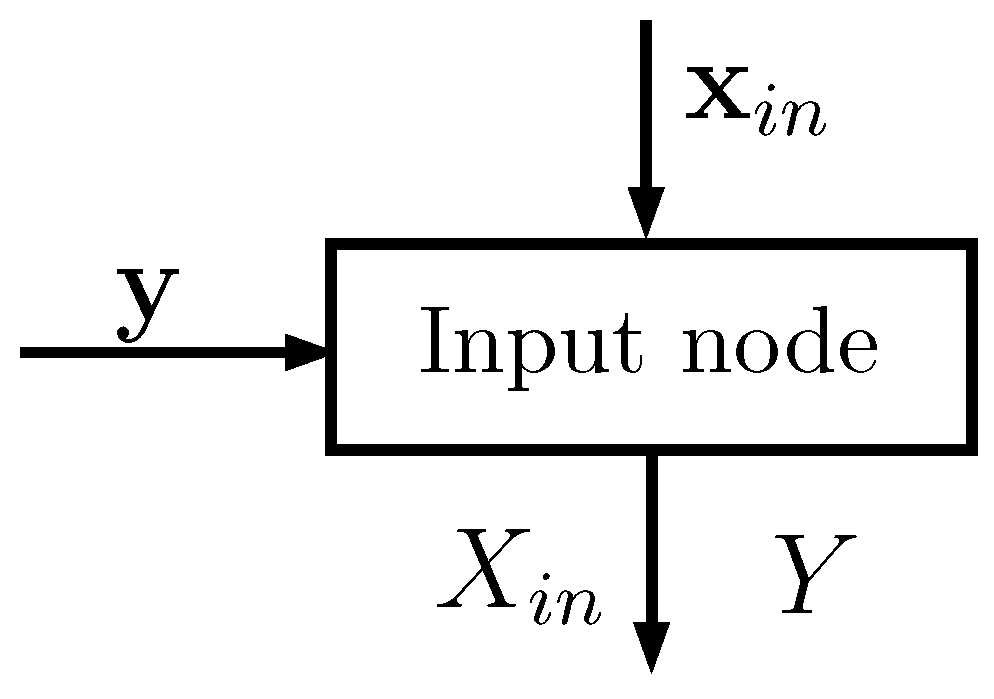
2.1. The Input Node
Each input node (see
Figure 1) has two input vectors:
of size , whose elements take values in a set of cardinality ; corresponds to one of the D features of the dataset (typically one column)
of size , whose elements take values in a set of cardinality ; corresponds to the known classes of the points
The notation we use in the equations below is the following:
represent random variables;
and
are the
nth elements of vectors
and
, respectively; and
is equal to 1 if
c is true, and is otherwise equal to 0. Using Laplace smoothing [
2], the input node estimates the following probabilities (the probability mass function of
Y in Equation (
1) is common to all the input nodes: it can be evaluated only by the first one and passed to the others):
From basic application of probability rules, and are then computed. From now on, for simplicity, we denote all the estimated probabilities simply as P.
All the above probabilities can be organized in matrices defined as follows:
Note that vectors and are not needed by the subsequent elements in the tree; only the input nodes have access to them.
Notice also that the following equalities hold:
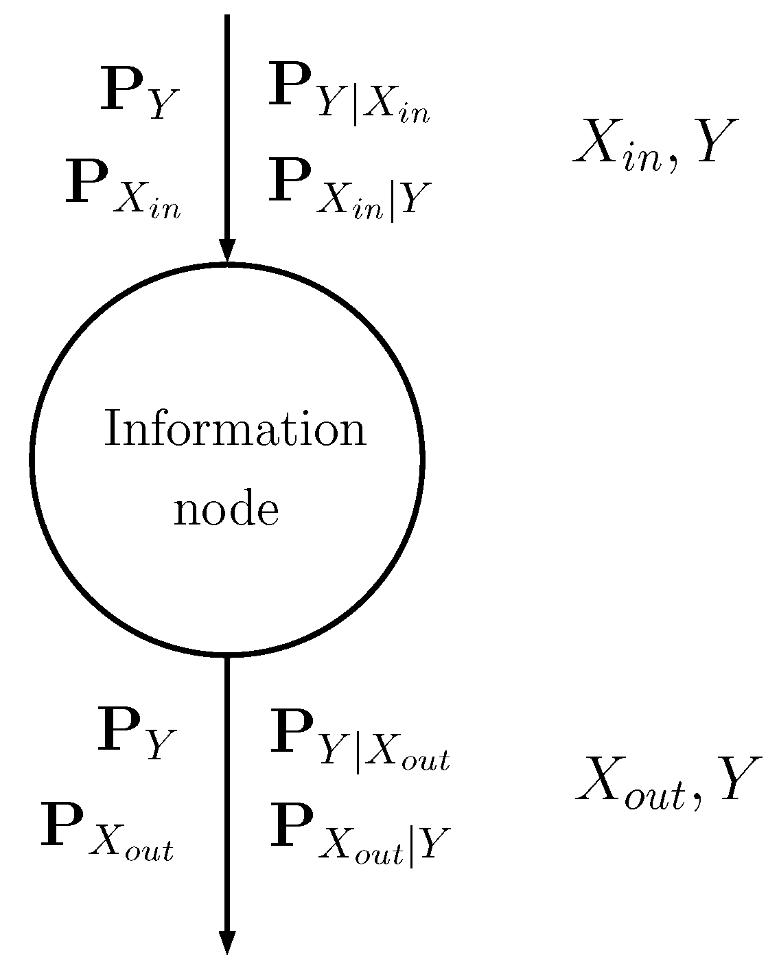
2.2. The Information Node
The information node is schematically shown in
Figure 2: the input discrete random variable
is stochastically mapped into another discrete random variable
(see [
16] for further details) through probability matrices:
The input probability matrices describe the input random variable , with possible values, and its relationship with class Y.
The output matrices describe the output random variable , with possible values, and its relationship with Y.
Compression (source encoding) is obtained by setting .
In the training phase, the information node generates the conditional probability mass function that satisfies the following equation (see [
14]):
where
The probabilities
can be iteratively found using the Blahut–Arimoto algorithm [
14,
24,
25].
Equation (
10) solves the information bottleneck: it minimizes the mutual information
under the constraint of a given mutual information
. In particular, Equation (
10) is the solution of the minimization of the Lagrangian
If the Lagrangian multiplier
is increased, then the constraint is privileged and the information node tends to maximize the mutual information between its output
and the class
Y; if
is reduced, then minimization of
is obtained (compression). The information node must actually balance compression from
to
and propagation of the information about
Y. In our implementation, the compression is also imposed by the fact that the cardinality of the output alphabet
is smaller than that of the input alphabet
.
The role of the information node is thus that of finding the conditional probability matrices
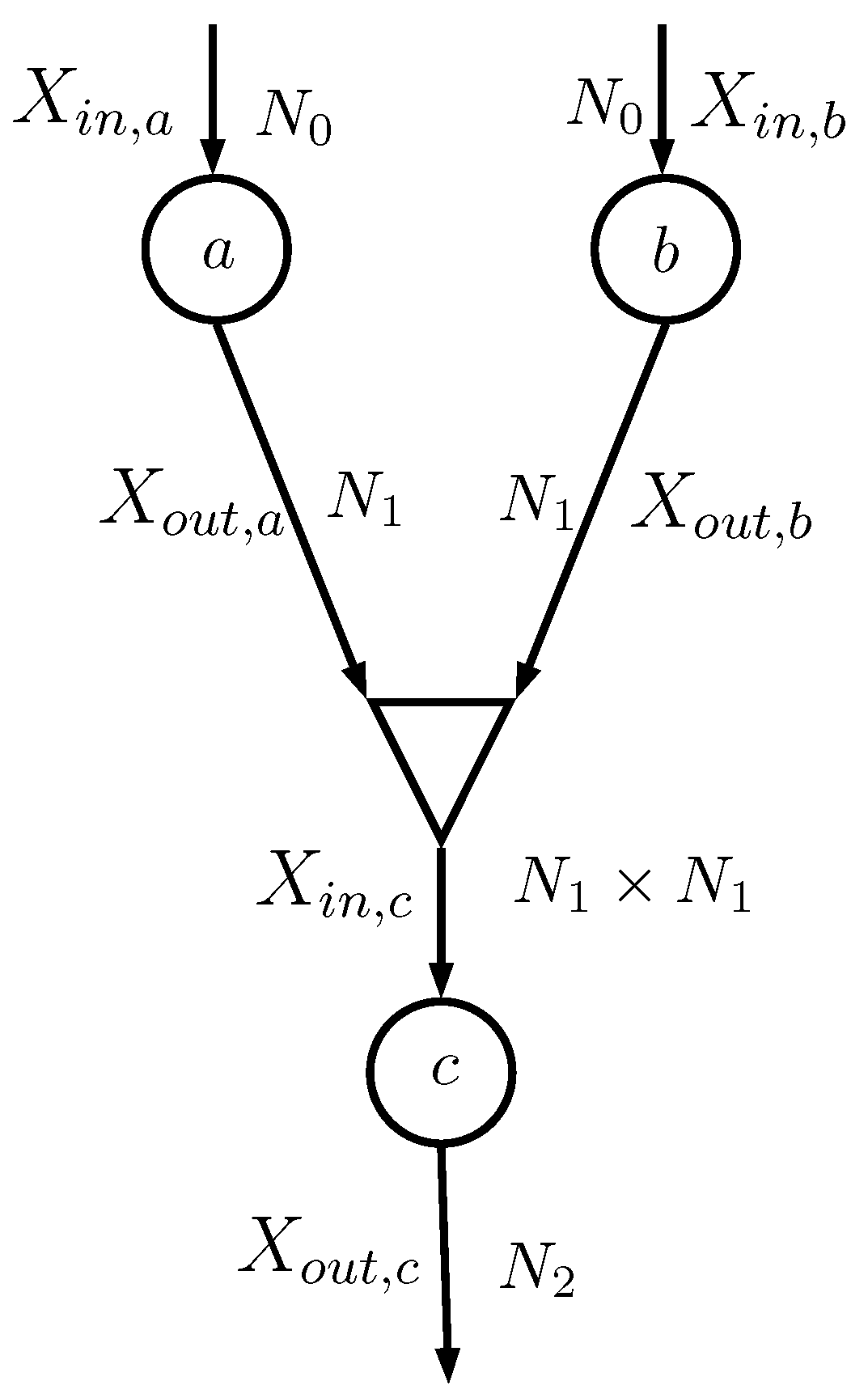
2.3. The Combiner
Consider the case depicted in
Figure 3, where the two information nodes
a and
b feed a combiner (shown as a triangle) that generates the input of the information node
c. The random variables
and
, both having alphabet with cardinality
, are combined together as
that has an alphabet with cardinality
.
The combiner actually does not generate
; it simply evaluates the probability matrices that describe
and
Y. In particular, the information node
c needs
, which can be evaluated
assuming that
and
are conditionally independent given
Y (notice that in implementation [
16] this assumption was not necessary):
where
. In particular, the
mth row of
is the Kronecker product of the
mth rows of
and
(here
identifies the
mth row of matrix
). The probability vector
can be evaluated considering that
so that
At this point, matrix
can be evaluated element by element since
It is straightforward to extend the equations to the case in which
and
have different cardinalities.
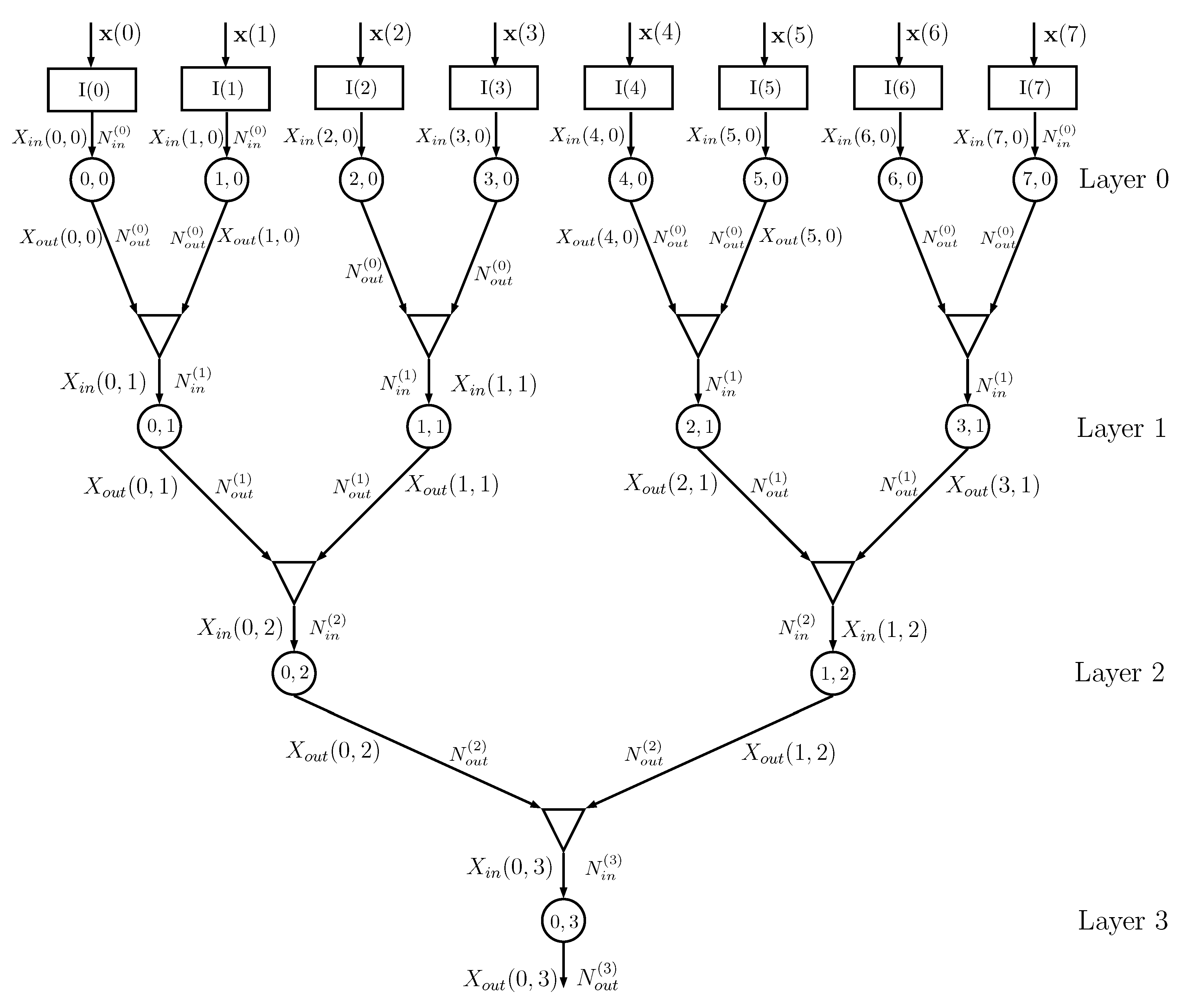
2.4. The Tree Architecture
Figure 4 shows an example of a DIN, where we assume that the dataset has
features and that training is thus obtained using a matrix
with
rows and
columns, with a corresponding class vector
. The
kth column
of matrix
feeds, together with vector
, the input node
,
.
Information node
at layer 0 processes the probability matrices generated by the input node
, with
possible values of
, and evaluates the conditional probability matrices with
possible values of
, using the algorithm described in
Section 2.2. The outputs of info nodes
and
are given to a combiner that outputs the probability matrices for
, having alphabet of cardinality
, using the equations described in
Section 2.3. The sequence of combiners and information nodes is iterated, decreasing the number of information nodes from layer to layer, until the final root node is obtained. In the previous implementation of the DINs in [
16], the root information node outputs the estimated class of the input and it is therefore necessary that the output cardinality of the root info node is equal to
. In the current implementation, this cardinality can be larger than
, since classification is based on the output probability matrix
.
For a number of features
, the number of layers is
d. If
D is not a power of 2, then it is possible to use combiners with 3 or more inputs (the changes in the equations in
Section 2.3 are straightforward, since a combiner with three inputs can be seen as two cascaded combiners with two inputs each).
The overall binary topology proposed in
Figure 4 requires a number of information nodes equal to
and a number of combiners equal to
All the info nodes run exactly the same algorithm and all the combiners are equal, apart from the input/output alphabet cardinalities. If the cardinalities of the alphabets are all equal, i.e.,
and
do not depend on the layer
i, then all the nodes and all the combiners are exactly equal, which might help in a possible hardware implementation; in this case, the number of parameters of the network is
.
Actually, the network performance depends on how the features are coupled in subsequent layers and a random shuffling of the columns of matrix
provides results that might be significantly different. This property is used in
Section 3.1 for building the ensemble of networks.
2.5. A Note on Computational Complexity and Memory Requirements
The modular structure of the proposed method has several advantages in terms of both memory footprint and computational cost. The considered topology in this explanation is binary, similarly to what is depicted in
Figure 4. We furthermore consider for simplicity cardinalities of the
D input features all equal to
and input/output cardinalities of subsequent layers information node to also be fixed constants
and
, respectively. As we show in the experiment (
Section 5), small values for
and
such as 2, 3, or 4 are sufficient in the considered cases. Straightforward generalizations are possible when considering inhomogeneous cases.
At the first layer (the input node layer), each of the D input nodes stores the joint probabilities of the target variable Y and its input feature. Each node thus includes a simple counter that fills the probability matrix of dimension . Both the computational cost and the memory requirements for this first stage are the same as the Naive Bayes algorithm. Notice that, from the memory requirements point of view, it is not necessary to store all the training data but just counters with number of joint occurrences of features/classes. If after training, new data are observed, it is in fact sufficient to update the counters and properly renormalize the values to obtain the updated probability matrices. In this paper, we do not cover the topic of online learning as well as possible strategies to reduce the computational complexity in such a scenario.
At the second layer (the first information node layer), each node receives as input the joint probability matrix of feature and target variable and performs the Blahut–Arimoto algorithm. The internal memory requirement of this node is the space needed to store two probability matrices of dimensions
and
, respectively. The cost per iteration of Blahut–Aritmoto depends on matrix multiplication of sizes
and
, and thus obviously the complexity scales with the number of classes of the considered classification problem. To the best of our knowledge, the convergence rate for the Blahut–Arimoto algorithm applied to information bottleneck problems is unknown. In this study, however, we found empirically that, for the considered datasets, 5–6 iterations per node are sufficient, as discussed in
Section 5.5.
Each combiner process the matrices generated by two information nodes: the memory requirement is zero and the computational cost is roughly Kronecker products between rows of probability matrices. Since for ease of explanation we chose the output probability matrix have again dimensions .
The overall memory requirement and computational complexity (for a single DIN) is thus going to scale as
D times the requirements for an input node,
times the requirements for an information node, and
times the requirements for a combiner. To complete the discussion, we have to remember that a further multiplication factor of
is required to take into account that we are considering an ensemble of networks (actually, at the first layer, the set of input nodes can be shared by the different architectures since only the relative position of the input nodes changes, see
Section 3.1).
5. Experiments
In this section, we analyze the results obtained with benchmark datasets. In particular, we consider the DIN ensemble when: (a) each DIN is based on the probability matrices (the scheme described in this paper); and (b) each information node of the DIN randomly generates the symbols, as described in the previous work [
16]. We refer to these two variants in captions and labels as DIN(Prob) and DIN(Gen), respectively. The reason for this comparison is that conditional statistical independence is not required in the case DIN(Gen), and the classification accuracy could be different in the two cases. Note that Franzese and Visintin [
16] considered just one DIN, not an ensemble of DINs. In the following, we introduce three datasets on which we tested the method (
Section 5.1,
Section 5.2 and
Section 5.3) and propose some examples of DINs architectures. Complete analysis of numerical results is described in
Section 5.4.
Section 5.5 and
Section 5.6 analyze the impact of changing the maximum number of iterations of Blahut–Arimoto algorithm and Lagrangian coefficient
, respectively. Finally, a synthetic multiclass experiment is described in
Section 5.7. In all experiments, the value of
was optimized similarly to what is described in
Section 5.6 using the training set.
5.1. UCI Congressional Voting Records Dataset
The first experiment on real data was conducted on the UCI Congressional Voting Records dataset [
27], which collects the votes given by each of the U.S. House of Representatives Congressmen on 16 key laws (in 1985). Each vote can take three values corresponding to (roughly, see [
27] for more details) yes, no, and missing value; each datum belongs to one of two classes (Democrats or Republican). The aim of the network is, given the list of 16 votes, decide if the voter is Republican or Democratic. In this dataset, we thus have
features and 435 data split into
data for training and
data for testing. The architecture of the used network is the same as the one described in
Section 2.4, except for the fact that there are 16 input features instead of 8 (the network has thus one more layer). The input cardinality in the first layer is
(yes/no/missing) and the output cardinality is set to
. From the second layer on, the input cardinality for each information node is equal to
and
. In the majority of the cases, the size of the probability matrices is therefore
or
. In this example, we used
and
(roughly 50% of the data). The value of
was set to 2.2.
5.2. UCI Kidney Disease Dataset
The second considered dataset was the UCI Kidney Disease dataset [
28]. The dataset has a total of 24 medical features, consisting of mixed categorical, integer, and real values, with missing values. Quantization of non-categorical features of the dataset was performed according to the thresholds in
Appendix A, agreed upon by a medical doctor.
The aim of the experiment is to correctly classify patients affected by chronic kidney disease. We performed 100 different trials training the algorithms using only out of 400 samples for the training. Layer zero has 24 input nodes, and then the outputs of layer zero are mixed two at a time to get 12 information nodes at Layer 1, 6 at Layer 2, and 3 at Layer 3; the last three nodes are combined into a unique final node. The output cardinality of all nodes is equal to . The value of was set equal to 5.6. In addition, in this case, we used an ensemble of DINs.
5.3. UCI Mushroom Dataset
The last considered dataset was the UCI Mushroom dataset [
29]. This dataset is comprised of 22 categorical features with different cardinalities, which describe some properties of mushrooms, and one target variable that defines whether the considered mushroom is edible or poisonous/unsafe. There are 8124 entries in the dataset. We padded the dataset with two null features to reach the cardinality of 24 and used exactly the same architecture as the kidney disease experiment. We selected
,
, and number of DINs equal to
.
5.4. Misclassification Probability Analysis
We hereafter report results in terms of misclassification probability between the proposed method and several classification methods implemented using MATLAB
® Classification Learner. All datasets were randomly split 100 times into training and testing subsets, thus generating 100 different experiments. The proposed method shows competitive results in the considered cases, as can be observed in
Table 1. It is interesting to compare in terms of performance the proposed algorithm with respect to the Naive Bayes classifier, i.e., Equation (
34), and the Bagged Tree algorithm, which is the closest algorithm (conceptually) to the one we propose. In general, the two variants of the DINs perform similarly to the Bagged Trees, while outperforming Naive Bayes. For Bagged Trees and KNN-Ensemble, the same number of learners as DIN ensembles were used.
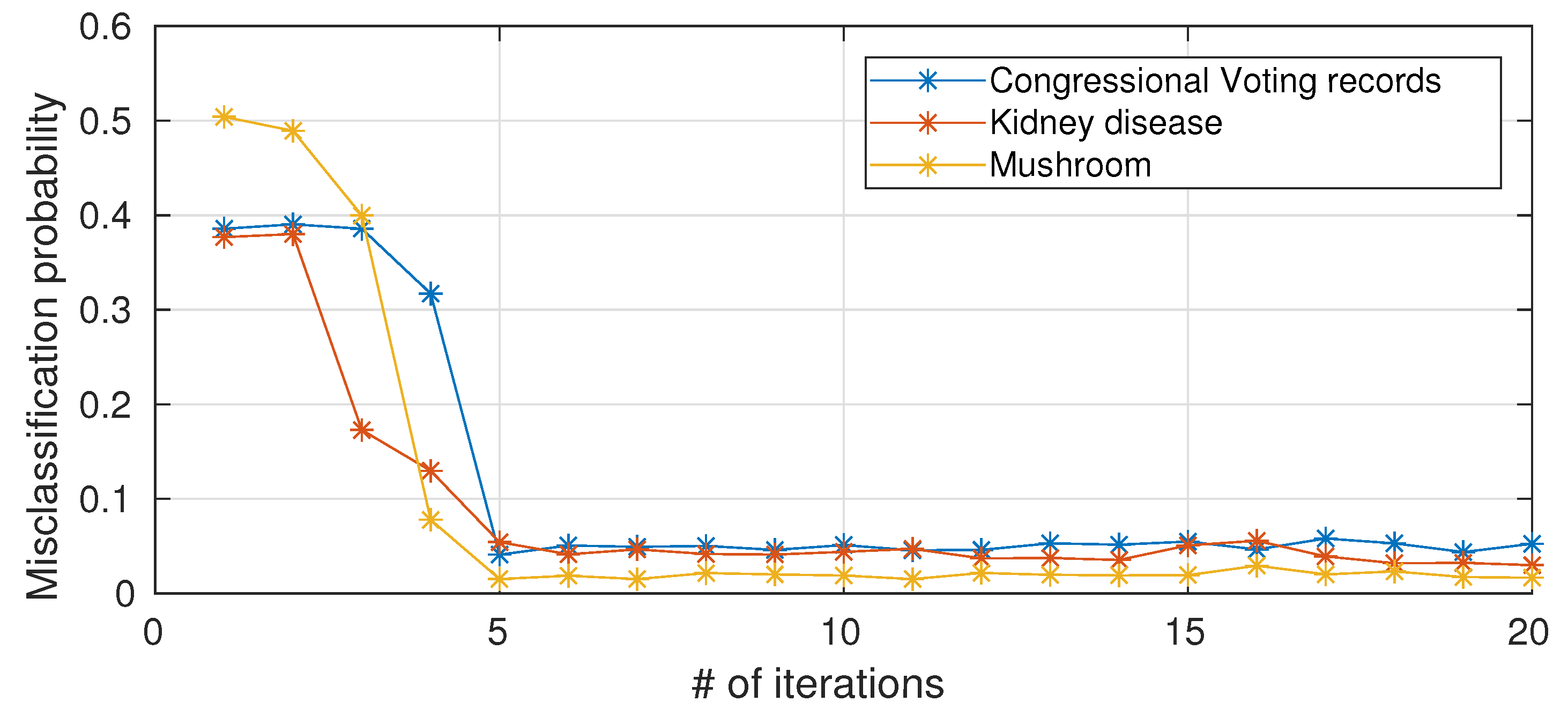
5.5. The Impact of Number of Iterations of Blahut–Arimoto on The Performance
As anticipated in
Section 2.5, the computational complexity of a single node scales with the number of iterations of Blahut–Arimoto algorithm. To the best of our knowledge, a provable convergence rate for the Blahut–Arimoto algorithm in the information nottleneck setting does not exist. We hereafter (
Figure 5) present empirical results on the impact of limiting the number of iterations of Blahut–Arimoto algorithm (for simplicity, the same bound is applied to all nodes in the networks). When the number of iterations is too small, there is a drastic decrease in performance because the probability matrices in the information nodes have not yet converged, while 5–6 iterations are sufficient and a further increase in the number of iterations is not necessary in terms of performance improvements.
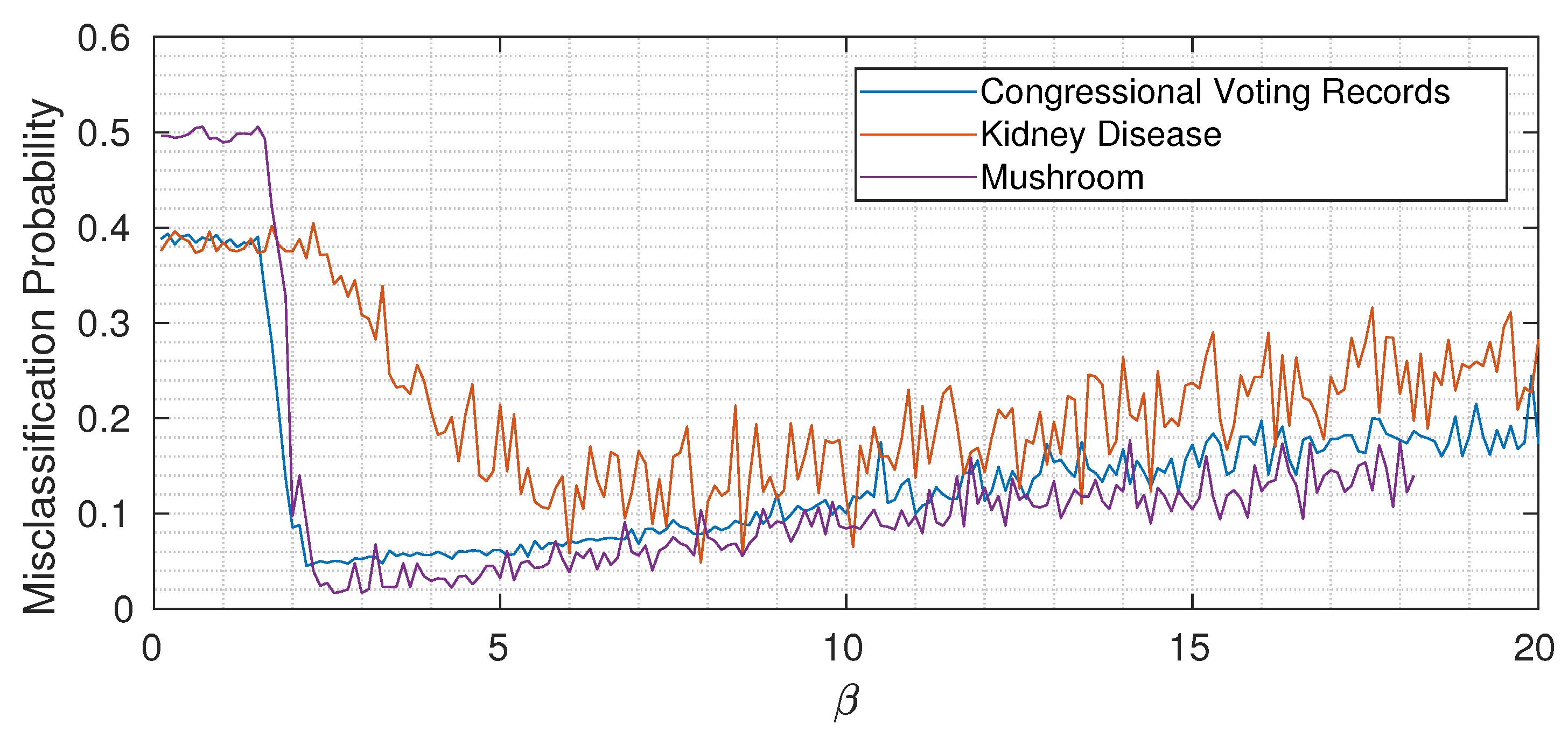
5.6. The Role of : Underfitting, Optimality, and Overfitting
As usual with almost all machine learning algorithms, the choice of hyperparameters is of fundamental importance. For simplicity, in all experiments described in the previous sections, we kept the value of
constant through the network. To gain some intuition,
Figure 6 shows the misclassification probability for different
for the three considered datasets (each time keeping
constant through the network). While the three curves are quantitatively different, we can notice the same qualitative trend: when
is too small, not enough information about the target variable is propagated, and then by increasing
above a certain threshold, the misclassification probability drops. Increasing
too much however induces overfitting, as expected, and the classification error (slowly) increases again. Remember (from Equation (
15)) that the Lagrangian we are minimizing is
Information theory tells us that at every information node we should propagate only the sufficient statistic about the target variable
Y. In practice, this is reflected in the role of
: when it is too small, we neglect the term
and just minimize
(that corresponds to underfitting), while increasing
allows passing more information about the target variable through the bottleneck. It is important to remember, however, that we do not have direct access to the true mutual information values but just to an empirical estimate based on a finite dataset. Especially when the cardinalities of inputs and outputs are high, this translates into an increased probability of spotting spurious correlations that, if learned by the nodes, induce overfitting. The overall message is that
has an extremely important role in the proposed method, and its value should be chosen to modulate between underfitting and overfitting.
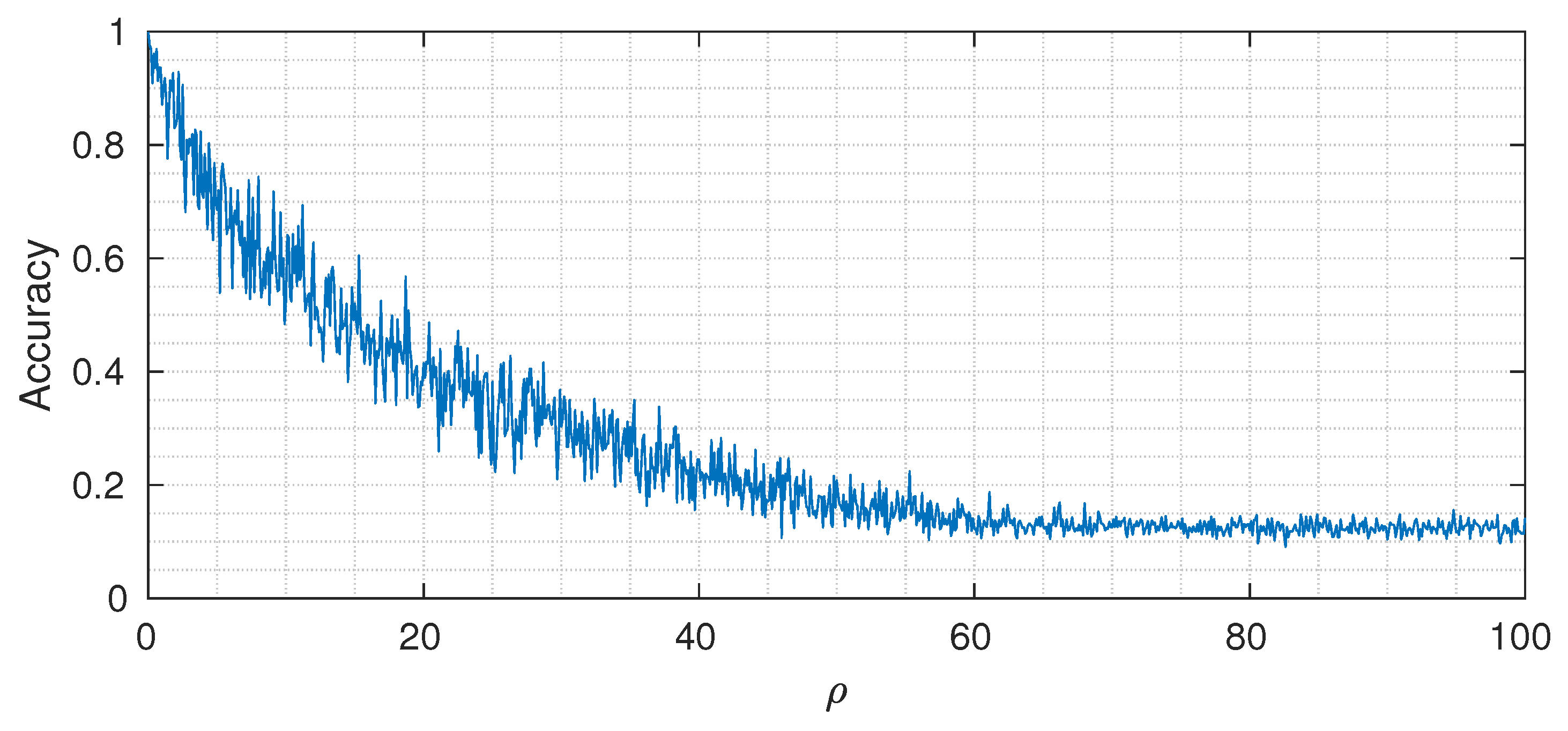
5.7. A Synthetic Multiclass Experiment
In this section we present results on a multiclass synthetic dataset. We generated 64-dimensional feature vectors
drawn from multivariate Gaussian distributions with mean and covariance depending on a target class
y and a control parameter
:
where for the considered experiment
. The mean
is sampled from a normal 64-dimensional random vector and
is randomly generated as
(where
is sampled from a matrix normal distribution) and normalized to have unit norm. The other parameter
is inserted to modulate the signal to noise ratio of the generated samples: a smaller value of
corresponds to smaller feature variances and more distinct, less overlapping, pdfs
, and an easier classification task. We then perform quantization of the result using 1 bit, i.e., the input of the ensemble of DINs is the following random vector:
where
is the Heaviside step operator. The designed architecture has at the first layer 64 input nodes, followed by 32, 16, 4, 2, and 1. The output cardinalities are equal to 2 for the first three layers, 4 for the fourth and fifth layer, and 8 at the last layer. We selected
,
(constant trough the network), and number of DINs equal to
.
Figure 7 shows the classification accuracy (on a test set of 1000 samples) for different values of
. As expected, when the value of
is small, we can reach almost perfect classification accuracy, whereas, by increasing it, the performance drops to the point where the useful signal is completely buried in noise and the classification accuracy reaches the asymptotic level of
(that corresponds to random guessing when the number of classes is equal to 8).
6. Conclusions
The proposed ensemble Deep Information Network (DIN) shows good results in terms of accuracy and represents a new simple, flexible, and modular structure. The required hyperparameters are the cardinality of the alphabet at the output of each information node, the value of the Lagrangian multiplier , and the structure of the tree itself (number of input information nodes of each combiner).
Simplistic architecture choices made for the experiments (such as equal cardinality of all node outputs, constant through the network, etc.) performed comparably to finely tuned networks. However, we expect that, similar to what happened in neural network applications, a domain specific design of the architectures will allow for consistent improvements in terms of performance on complex datasets.
Despite the local assumption of conditionally independent features, the proposed method always outperforms Naive Bayes. As discussed in
Section 4, the induced equivalent probability matrix is different in the two cases. Intuitively, we can understand the difference in performance under the point of view of probability matrix factorization. On the one side, we have the true, exponentially large, joint probability matrix of all features and target class. On the other side, we have the Naive Bayes one, which is extremely simple in terms of complexity but obviously less performing. In between, we have the proposed method, where the complexity is still reasonable but the quality of the approximation is much better. The DIN(Gen) algorithm does not require the assumption of statistical independence, but the classification accuracy is very close to that of DIN(Prob), which further suggests that the assumption can be accepted from a practical point of view.
The proposed method leaves open the possibility of devising a custom hardware implementation. Differently from classical decision trees, in fact, the execution times of all branches as well as the precise number of operations is fixed per datum and known a priori, helping in various system design choices. In fact, with classical trees, where a node’s utilization depends on the datum, we are forced to design the system for the worst case, even if in the vast majority of time not all nodes are used. Instead, with DIN, there is no such a problem.
Finally, a clearly open point is related to the quantization procedure of continuous random variables. One possible self-consistent approach could be devising an information bottleneck based method (similar to the method for continuous random variables [
20]).
Further studies on extremely large datasets will help understand principled ways of tuning hyperparameters and architecture choices and their relationship on performance.


