1. Introduction
As a nonlinear dynamical system, a diesel generator’s safe and smooth running is essential to the reliability of systems. The gearbox is a core part of a diesel generator, directly determining its performance. Remaining Useful Life (RUL) prediction can detect faults early and estimate the downtime of diesel generator components, further helping operators to arrange a reasonable maintenance schedule and save operating costs.
Vibration signal analysis is one of the most widely used methods of condition monitoring. Vibration monitoring generally involves arranging sensors at important locations, using the data acquisition card to obtain signals, and finally using the computer to calculate and analyze the data. This article aims at analyzing the degradation trend of machines and predicts their RUL with the vibration signal collected from the sensors online or offline. In this way, the RUL of a diesel generator is achieved during condition monitoring.
One of condition-based maintenance (
CBM)’s main missions is to predict a machine’s
RUL [
1].
RUL prediction counts more than fault diagnosis in the makings of maintenance decisions [
2]. According to the data and continuous degradation trend recorded by the condition detection system,
RUL is predicted. It will forecast a potential degradation when current faults have been cleared, providing direct references for
CBM. As
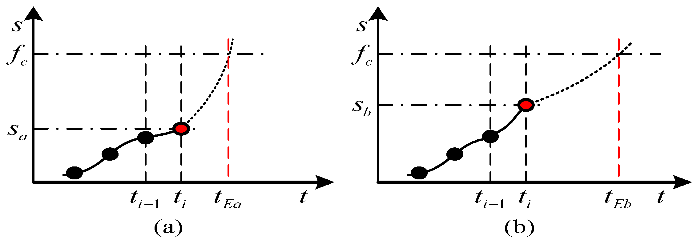
Figure 1 shows, the functional degradation of
a and
b stands at an even level at
ti−1.
Sa,
Sb represent the degree of performance degradation for machine
a and
b, and
fc means that the machine is incapable of working. Additionally, at
ti,
a’s health level is higher than
b’s, indicating that
a is healthier. After
ti,
a’s function degrades faster than
b’s and
a’s
RUL is shorter. Any planned maintenance must be performed on
a in advance [
3].
RUL is defined as the time span from the present moment to the end of the useful life [
4], expressed as
, where
tEol is life termination,
tk is the present moment, and
is the remaining life at
tk.
The primary mission of
RUL prediction is to monitor the useful time left before the system loses its working capability according to condition detection information. Based on time series analysis, the accuracy of prediction is the primary factor considered in the choice of prediction method. The existing methods are based on physical models, statistical data, and artificial intelligence [
5], as described in the following:
(1)
RUL prediction methods based on physical models reflect the life-cycle degradation process of the system by establishing a mathematical model based on the failure mechanism [
5]. As a typical physical model, the Paris-Erdogan model (PE) is widely used for
RUL prediction. Frank et al. [
6] used PE to predict the
RUL of two types of pipelines, 80 and 100. Hu et al. [
7] used Norton’s law to describe the creep of a turbine and combined the Kalman filtering (
KF) and particle filter (
PF) to predict
RUL; however, the methods based on physical models need the deep understanding and sufficiently accurate judgment of failure mechanism to ensure the accuracy of RUL estimation.
(2) RUL prediction methods based on statistical data fit the observational data into a random coefficient model and a stochastic process model. This method is widely applied as many on-the-shelf statistical models can be applied to fit the data, that is for instance random coefficient models, autoregressive models, Gamma process models, inverse gaussian processes, Markov models, and proportional hazards models. However, Autoregressive models rely heavily on high-quality historical data and are not conducive to RUL prediction under complex operating conditions, Wiener models and Gamma process models is limited by the assumption of Markov, which assume that the future state is only related to the current state but not to the past state, so it is not applicable to some practical situations.
(3)
RUL prediction methods based on artificial intelligence concentrate on learning the degradation pattern of the system from observations. Common
AI techniques include the artificial neural network (
ANN), neural fuzzy (
NF), support vector machine/relevance vector machine (
SVM/RVM), K-nearest neighbor (
KNN) and Gaussian process regression (
GPR). Hussain et al. [
8] extracted the index of health from the vibration signal, and established the
RUL prediction model by the adaptive neural fuzzy inference system and nonlinear autoregression. The
NF excels in
RUL prediction because it takes advantage of expert knowledge and intelligent
ANN, but needs high-quality data sources. There are many different kinds of
SVM that are used for machines’
RUL prediction, like one-class
SVM and multi-class
SVM [
9], and Squares-
SVM [
10]. However,
SVM only provides point estimate and does not provide a probability distribution over of points. In order to make up for this shortcoming,
RVM was proposed, which has the same functional form as
SVM, but provides a full probability distribution over all possible outcomes [
11]. However, those methods focus more on data training rather than analysing the mechanism of mechanical failure. The structure and parameters of
ANN need to be set artificially, which leads to low generalization ability; Kernel function selection for SVM/RVM with different objects is a huge challenge. Calculation process of GPR is complex and takes a long time.
It can be seen from the above that the three
RUL prediction ideas have their own limitations. The methods of
RUL prediction are variable, among which, similarity measure of the data-driven prediction is advantageous at avoiding constructing complex functional degradation models. Therefore, this paper will study
RUL prediction based on statistical data from the perspective of similarity measure. Research on similarity-based
RUL prediction was first proposed in 2012 and has been proved to be a very effective RUL prediction approach [
12,
13,
14,
15,
16]. However, the methods have not been so widespread until now. The basic idea is that products with similar degradation processes have a similar service life [
3]. The
RUL of the test sample is determined by observing the similarity between the performance degradation trajectory of the test sample and the reference samples of the known life-cycle degradation process.
There is little literature about RUL prediction based on similarity but they verified the validity of “similarity” idea. You et al. [
12] conducted an experiment to predict the
RUL of a welding spot under vibrations. He thought if the asset under study is more similar to reference sample “A”, then “A” should play a more important role in RUL estimation of the asset under study. Eker [
13] testified the function of similarity-based prediction through data collected from Virkler’s fatigue crack propagation, a degradation data set of drilling, and a turnout system of slide chair degradation. Zhang [
14] put forward a method to predict the
RUL of a mechanical system based on the similarity of a phase space trajectory and found that the results approximated the actual
RUL very closely. Xiong [
15] built a one-dimensional damage indicator on an aero engine’s multiple parameters by means of liner regression. He obtained the
RUL after matching test engine data to the model base. In the same way, Moghaddass [
16] adopted principal components analysis to integrate a turbine engine’s multiple parameters and drew the first principal component to describe the system degradation process.
It can be concluded from the literature review that similarity-based
RUL prediction methods so far are almost always built on a single parameter. The latest research is only employed to integrate multiple parameters into a one-dimensional parameter firstly, and then compare the similarity of performance degradation curves with statistical methods or
AI methods. There is no research about co-impact both multiple samples and multiple parameters of those samples on
RUL prediction. However, performance degradation or malfunction may result from a multitude of reasons. Thus, multiple parameters of different perspectives may provide a more comprehensive reflection of the running process [
17]. Especially for a complex system, what a single parameter can present is far less than multiple parameters in describing the degradation of various forms.
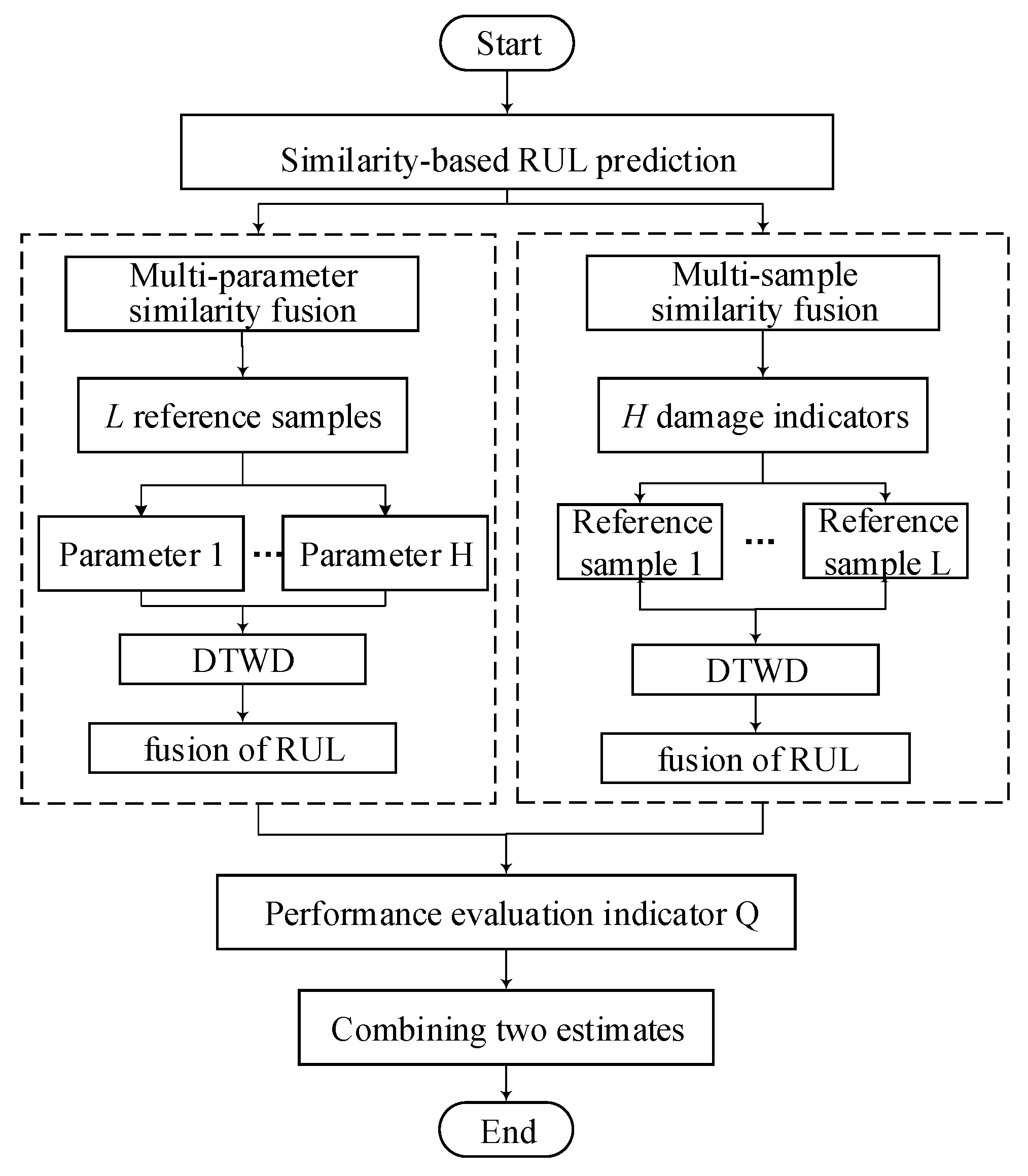
Therefore, this paper proposes an RUL prediction method based on the similarity fusion of multiple damage indicators and samples. In contrast to the more traditional methods, the method of multi-parameter and multi-sample similarity fusion estimates RUL by referring to multiple parameters and samples.
The process can be divided into five parts. At first, in
Section 2.1 and
Section 2.2, the various time and frequency domain features extracted from a vibration signal that will be applied as damage indicators are introduced together with the entropy variance method for fuzzy filtering applied for low pass filtering of the time-domain features. Further, the method used for parameter evaluation in order to select the most significant performance damage indicators to be applied for RUL prediction is discussed. Second, in
Section 2.3, we introduce principles of
RUL prediction based on similarity and defines four core elements in the
RUL prediction based on similarity: Time window
D, similarity measurement function
S(.), weight function
w(.), and performance evaluation indicator
Q. Third, in
Section 2.4, we introduce the Dynamic Time Warping Distance (
DTWD) as the similarity measure function
S(.) to discuss the similarity of data degradation trajectory patterns for the first time. Fourth, in
Section 2.5,
Section 2.6 and
Section 2.7, according to combinations of different performance damage indicators, the
RUL prediction model based on the similarity fusion of multi-parameter and multi-sample methods is established. Finally, in
Section 3, this paper studies a type of heavy high-speed diesel generator produced by the China Shipbuilding Industry Corporation (
CSIC), and validates the
RUL prediction method proposed here with experimental results. In the meanwhile, Proposed method here are compared with the mature methods of Multivariable Support Vector Machine (
MSVM) and Principal Component Analysis (
PCA) for comparison analysis in
Section 3.3 and
Section 3.4.
2. Methodology
At first step, we will select the most significant performance damage indicators which will be the input of RUL estimation from various time and frequency domain features. Then, we will define four core elements in the RUL prediction based on similarity: Time window D, similarity measurement function S(.), weight function w(.), and performance evaluation indicator Q. Next, as the most important core, similarity measurement function S(.) will be established with DTWD and we write the details about DTWD in
Section 2.3. At last, the RUL prediction model based on the similarity fusion of multi-parameter and multi-sample methods will be established.
2.1. The Damage Indicators
The various time domain and frequency domain features extracted from the vibration signal will be used as damage indicators in the following RUL prediction. Further, we discuss the method we apply to to define for each individual gearbox under study a subset of most significant damage indicators system, to be applied for RUL prediction for this particular gearbox. The time domain features of the vibration signal effectively reflect the performance degradation of the gearbox [
18]. As shown in
Table A1 of
Appendix A, we have chosen to use 10-time domain features as damage indicators [
19]. Further, the Fourier transform is applied to convert the vibration signal into its frequency spectrum representation [
20]. We have chosen to use 15 frequency domain features [
21], as damage indicator, see
Table A2 in
Appendix A.
Since the time-series of the various damage indicators are noisy and in order to correctly compare them with the reference samples we need to smooth the series, i.e., low pass filtering. Fuzzy filtering is a low pass filtering method based on fuzzy set theory, which can adjust the filter structure adaptively based on the features of the signal [
22]. A large number of studies have shown that this method is easy to implement and has a good filtering effect, which is very suitable for engineering applications.
For time domain features, this paper proposed the low pass filtering based on approximate entropy variance. The time-series of the various damage indicators are rather noisy, we apply low pass filtering techniques to smooth them [
23]. For the time domain damage indicators we have applied low-pass filtering with approximate entropy variance (Aev), because approximate entropy [
24] is suitable for describing dynamic noise with a small amount of data and has a strong Robustness to observation noise, and the dynamics system is easy to reconstruct. Approximate entropy variance is a statistic measuring the complexity of time series and it can accurately measure the complexity of signals. Especially in the case of small data quantity and noise interference, it also demonstrates statistical stability. The variance could describe the stability in time series. Approximate entropy (
Ae) is defined as: For time series
,
x(
i) denotes
m consecutive values of
u starting at point
i:
where:
H() is the Heaviside function, After
Ae is calculated,
Aev is defined as:
Then low-pass filtering decomposes the damge indicator signal into the parts trend and noise:
With
X(
tk) is the value of the performance damage indicator at time
tk,
XT(
tk) is the trend term,
XR(
tk) the noise term, and
tk = 1, 2,…,
N, with
N the number of discrete observations made within the measurement time interval.The weighting filter and fuzzy filtering membership function are defined as
according to [
24], the range of u’(x
n−k) is a [0, 1], and
f is set to normal distribution function. So XT(t
k) will be ramained while XR(t
k) removed.
To smooth the frequency domain damage indicator over time, a simple moving average filtering is applied. The moving average filtering can reduce random noise while reflect unit step function response of signal [
25]. First, the damage indicators are decomposed into two parts just as before in Equation (5), then calculate the average value as the predicted value of the next sub-interval and move forward in turn.
is the first part of damage indicator with moving average filtering which is defined as the weighted average value of the adjacent
N data points.
In
Figure 2, as an example of the full signal together with its trend is shown for one of the time/frequency domain indicators. The ideal output can be obtained by wave filtering.
2.2. Defining a Subset of Most Significant Damage Indicators
To define an—asset dependent—subset of most significant damage indicators to be applied for RUL prediction of the asset, so called significance indicators have been defined [
26]. By aid of these significance indicators each of the twenty-five damage indicators is evaluated and a score from 0 to 1 is given to each damage indicator as a measure of how significant the parameter is for the RUL prediction for the asset under study. We have defined three significance indicators, Correlation, Monotonicity and Robustness to act as RUL significance indicators, and which will be defined and explained in the following.
The correlation r measures the correlation of a damage indicator with time (that is over the whole time span the vibration measurements have been performed), i.e., it states the normalized slope of the trend of the damage indicator over time, i.e., , with X is the damage indicator, σX the standard deviation of X, σt the standard deviation of the the variable t time, and b the slope of the regression line ‘found by linear regression when viewing X as a function of t.
The Monotonicity indicator reflects the unidirectional trend of time domain features and frequency domain features. The larger the value of Monotonicity, the greater the slope of the parameters, and the more intuitive and obvious the trend of performance degradation. If a parameter rises and falls recurrently in the degradation process, it may be just a cyclic change as the machine vibrates. That does not change in a certain direction as performance degradation occurs.
The Robustness indicator reflects the tolerability of damage indicators for outliers. Robustness measures whether the degradation parameter is capable of resisting random interference [
27]. If a parameter is sensitive to external disturbance, it does not contain valuable information even if it fluctuates wildly.
The equations applied to compute each of the indicator indicators are stated in
Appendix B.
This study proposes a combination function W with three indicators above as a “ruler” to select several optimal parameters for following RUL prediction.
In this equation,
W is the combination function, distributed in the range of [0, 1];
Ω represents a set of candidate damage indicators; and
ωi represents the weight of each indicator. The parameter with a larger value of
W should be selected for effective
RUL prediction.
ωi is determined by two sources: Subjectively, due to the fact that damage indicator is used to describe performance degradation trajectory as time goes,
Mon should take up the largest weight. This is in compliance with similarity-based prediction method. So
ωi will be subjectively assigned a value denoted as prior weighing
ai. While objectively, the optimal combination of the chosen damage indicators in essence is about constrained optimization. We adopt the solving model with
AMPL, input the permutation and combination of three indicators’ weights (adjustment of weighting is from 0.2~0.8), and determine the posterior weighting
bi. according to the results. At last, considering both prior weighing
ai and posterior weighting
bi,
ωi will be determined, and some more significant damage indicators can be chosen for subsequent
RUL estimation.
2.3. Similarity-Based RUL Prediction
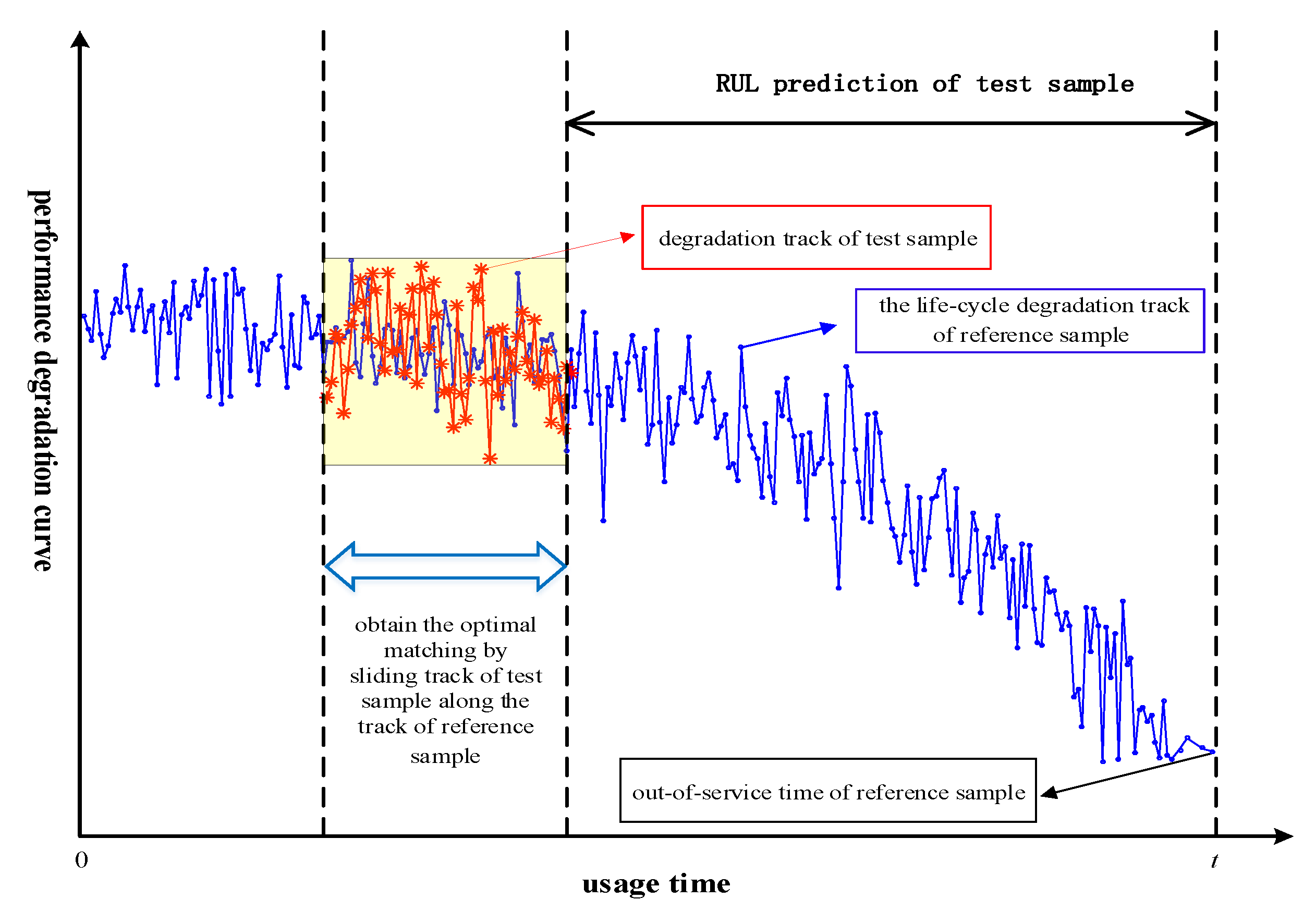
As
Figure 3 shows, the concept of the similarity-based RUL prediction method is that assets that show similar behavior of their damage indicators have similar RUL values [
28]. By comparing the damage indicator time series of an asset with corresponding historical reference time-series, the RUL of the asset can be predicted. It is assumed that the assets from which reference indicator curves are available are the same or of closely related type of product or system—and have performed under more or less similar operating environments and conditions—as the asset under study.
The blue curve represents the time-series of one of the damage indicators over time for a reference gearbox, while the red curve is the time-series of same indicator for a gearbox in use on which we wish to make an RUL prediction. Now the similarity concept states that we should find the most similar certain part of blue curve to red curve, which named ‘optimal match’. When an optimal match has been established then as estimate for the RUL of gearbox of interest the length of the time interval of the blue curve which is on the right of the red is applied. Here we always assume that the final available measurement point of any of the reference curves corresponds with the end of the remaining useful life of the reference gearbox.
To apply the similarity prediction method, its four core elements need to be defined. These are the time window
D, the similarity measure function
S(.), a weight function
w(.), and the performance evaluation indicator
Q. The time window
D refers to the time interval of similarity between the test sample and reference samples, shown as the data block length marked as yellow in
Figure 3. The similarity measurement function
S(.) quantifies the similarity of the degradation trajectory of the test sample and reference samples. This paper will establish the
DTWD-based nonlinear dynamic programming algorithm as
S(.) which will be explained in
Section 2.4. The weight function
w(.) concerns the similarity between the test sample and reference samples, and it gives different weights to different reference samples and different parameters in line with their contributions. The performance evaluation indicator
Q is used to describe differences between the
RUL estimated value and its actual value, which helps to find the optimal method through comparing different
RUL prediction methods. We borrowed 5 indicators as the performance evaluation indicator
Q, which are shown in
Appendix B (2).
Similarity-based RUL prediction follows four steps:
- (1)
Define the time window D to be used for each of the damage indicators related to an asset. The right side of the data block is the state of asset under study. The red curve is the time window D of the test sample and the blue curve is the life-cycle degradation state of reference sample. The right boundary line of D is observation point at present for test sample.
- (2)
Define a similarity measure function S(.) through which the similarity or closeness between two time-series is defined. DTWD algorithm is established as the similarity measure function S(.) in order to find the most similar part in one certain reference asset with the time window D, so one similarrity distance could be obtained. Suppose H most significant damage indicators are selected and L reference assets are compared with the asset under study, which means each reference asset contains H damage indicators. Then H*L similarity distances between each damage indicator in the asset under study and each damage indicator in those reference assets could be obtained by DTWD algorithm.
- (3)
Based on the thought “the more similar the two-time series is, the larger the weight value is”, we will make weighted summation among those H*L similarity distances. That is normalizing H*L similarity distances and then assigning different weights according to the thought such as closer distances will be given greater weights. The details of weight function w(.) based on multi-parameter and multi-sample refers to Equations (12) and (14) and Equations (16) and (18), respectively.
- (4)
For those RUL values referring to different parameters or different samples, weighted average method is used to obtain the test sample’s RUL estimation based on the corresponding weights calculated in step (3).
2.4. Similarity Measurement Function S(.): Dynamic Time Warping Distance (DTWD)
The
DTWD is a dynamic nonlinear programming idea, and an algorithm that matches time dimension warping with distance optimization planning [
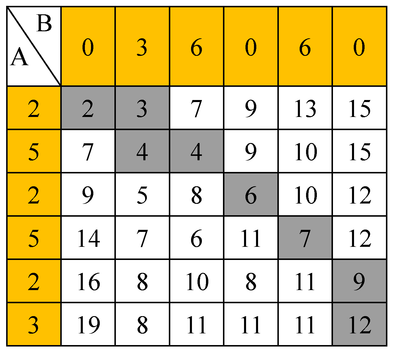
29]. DTWD has been widely used in text data matching, voice information processing and other fields in recent years. Compared with the traditional Euclidean distance, it shows better recognition accuracy and robustness in the application of time series. DTWD can compress and bend time series, make the overall distance of two sequences smaller. The DTWD of two time series is defined as the minimum distance between the two series calculated by time dimension bending. when calculating the distance between series A and B, traditional Euclidean Distance takes the distance between two time series A and B at same time point, while DWTD takes the distance between two time series A and B that needn’t at same time point in order to obtain the shortest distance. For example, supposing that time series A = {2,5,2,5,2,3}, B = {0,3,6,0,6,0}, so the traditional Euclidean Distance is calculated as 2 + 2 + 4 + 5 + 4 + 3 = 20, and DTWD is calculated as
Figure 4. The gray elements from the upper left corner to the lowest right corner are dynamic time warping path. The lowest right corner element ”12” is the cumulative distance D
twd(A,B) = 12.
Therefore, DTWD is calculated as follows: Setting time series A = (a1,a2,…,al) and B = (b1,b2,…,bj…,bk), l and k represent the sequence length of A and B, respectively. The DTWD algorithm needs to first align two time series and establish a l × k matrix D which contains the value d(ai,bj) on its ij-th entry. d (ai,bj) represents the distance between points ai and bj in two time series.
In matrix D, P (P = q1,q2,…,qn,…,qN) denotes the dynamic time warping path of time series A and B, qi represents the distance of time series A and B at time point i. Path P needs to meet the following four restraint conditions:
- (1)
Boundedness: max(l,k) < N < l + k−1;
- (2)
Boundary conditions: q1 = D(1,1) and qN = D(l,k), that is, the start and end points of the dynamic warping path can only be on the diagonal of the matrix;
- (3)
Continuity: For qn = (a,b) and qn−1 = (a’,b’), the conditions and must be met;
- (4)
Monotonicity: For qn = (a,b) and qn−1 = (a’,b’), a − a’ = 0 and b − b’ = 0 can’t happen. that is, all line segments representing the dynamic bending paths cannot intersect each other.
For small-scale data, an exhaustive search method can be used to find an optimal dynamic time warping path. For large-scale data, based on the Dynamic Programming Model, the optimal dynamic time warping path can be obtained by a recursive search algorithm with the local optimal solution from point (1,1) to point (
i,
j). Using
DTWD to represent
DTWD between time series
A and time series
B, the computation process is
In the equation,
p denotes the norm, rest(A) = {
a2, a3…
al}, rest(B) = {
b2, b3…
bk}. As Equation (9) showed,
d(ai,
bj) represents the first point’s distance between two time series, then search for each shortest bending path at each rest point(i.e., rest(A) and rest(B)) between two series. The pseudocode of
DTWD algorithm is shown in
Appendix B (3).
2.5. RUl Estimation by Multi-Parameter Fusion
Multi-parameter similarity fusion focuses on the impact of different parameters on the RUL estimation of the asset under study. As the four steps showed in
Section 2.3, Suppose
H most significant damage indicators are selected and
L reference assets are compared with the asset under study, which means each asset contains
H damage indicators. Then
H*L similarity distances between each damage indicator in the asset under study and each damage indicator in those reference assets could be obtained by
DTWD algorithm. First, according to the weight idea in step (3) of
Section 2.3, different weights are arranged to those
H*L similarity distances. Second, for each certain damage indicator H
i, we make weighted summation among those
Hi from
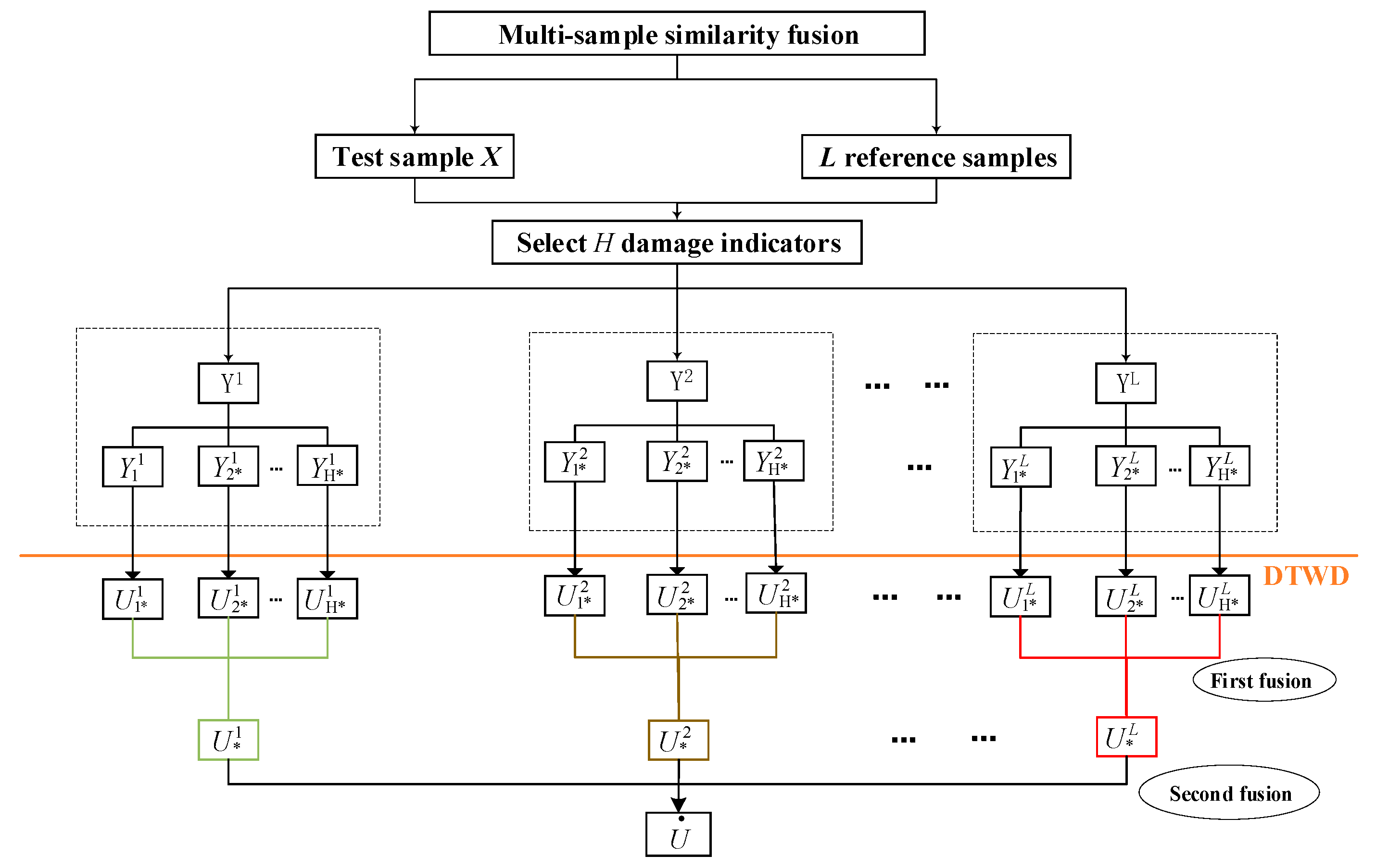
L reference assets respectively, which is called “first fusion” and need to be traversal
H times because there are total of
H damage indicators. After first fusion there will be
H similarity distances formed. Third, for those formed
H similarity distances, we make weighted summation among them again based on the weight idea in step (3). This is called “second fusion”. There will be one similarity distances formed called “RUL value”. At last, by finding the corresponding time point of “RUL value”, we can estimate the RUL.
The following is the calculation process of mathematical theory:
For a diesel generator gearbox, with a asset under study(called “test sample’) of
X, suppose
H performance damage indicators can be obtained with the method in
Section 2.2. With the
l-th reference sample
Yl,
l is the label of reference sample and
L is the number of reference samples. The idea of multi-parameter similarity fusion is shown in
Figure 5.
In
Figure 5, by
we denote the time-series of the
h-th damage indicator of the
l-th reference gearbox, with
l = 1,…,
L, and
L the total number of reference gearboxes. Further,
represents the RUL estimation described by the
h-th damage indicator of the
l-th reference sample, and
represents the
RUL value estimated by the
h-th damage indicator after first fusion.
(1) Calculating similarity distance between each damage indicator in the asset under study and each damage indicator in those reference assets which is denoted by
, so we need to run this step
H*L times and obtain total of
H*L similarity distances. let
denotes the optimal similarity distance by DTWD between the
h-th damage indicator of the
l-th reference sample and the
h-th damage indicator of the test sample. The calculation of
is as follows:
As
Figure 3 shows, we need to match the red block such that is most similar (w.r.t. a certain measure) to a part of the blue curve, that is to find an ‘optimal match’. Only when the
Dtwd attains a minimum, we can conclude that the right boundary line of D which corresponds to a time point of reference sample reflects the RUL of test sample. With the minimum of distance
is determined, the
is determined.
(2) First fusion:
represents the weight of
, so Equation (12) is established as weight function w(.) for the first fusion according to the idea” The smaller the distance between the two time series is, the larger the weight value of the parameter is.”, then
could be obtained as showed in
Figure 6.
and
have been calculated in Equations (10) and (11).
(3) Second fusion: After obtaining a total of
H ,
represents the weight of
, so Equation (14) is established as weight function w(.) for the second fusion.
2.6. RUl Estimation by Multi-Sample Fusion
Compared with multi-parameter similarity fusion, multi-sample similarity fusion focuses more on the similarity between reference assets and the asset under study, rather than the similarity among different parameters. Same as
Section 2.5, suppose
H most significant damage indicators are selected and
L reference assets are compared with the asset under study, which means each asset contains
H damage indicators. Then
H*L similarity distances between each damage indicator in the asset under study and each damage indicator in those reference assets could be obtained by
DTWD algorithm. First, according to the weight idea in step (3), different weights are arranged to those
H*L similarity distances. Second, for each certain reference sample
Li, we make weighted summation among those
Hi, which is called “first fusion” and need to be traversal
L times because there are total of
L reference samples. After first fusion there will be
L similarity distances formed. Third, for those formed
L similarity distances, we make weighted summation among them again based on the weight idea in step (3). This is called “second fusion”. There will be one similarity distances formed called “RUL value”. At last, by finding the corresponding time point of “RUL value”, we can estimate the RUL.
The following is the calculation process of mathematical theory:
- (1)
Repeating the steps (1) in
Section 2.5 based on multi-parameter similarity fusion;
- (2)
First fusion:
represents the weight of
, so Equation (16) is established as weight function w(.) for the first fusion, then
could be obtained as showed in
Figure 7. Unlike multi-parameter fusion, each reference sample is treated as a “unit”,
H damage indicators of a certain reference sample will have a fusion firstly in those units.
- (3)
Second fusion: For the obtained
, We used Equation (18) as weight function w(.) and make weighted summation to integrate L reference sample to the final RUL value
:
2.7. Combining the Two Estimates into One
After obtaining the two results of RUL estimation with two methods, it’s feasible to make “third fusion” to combining the two estimates into one. This paper provides another idea about combining yet. As
Figure 7 showed, the performance evaluation indicator Q is established to discuss the estimation results of the two methods, and the better RUL estimation result is selected for the diesel generator gearbox.
In addition, for a mechanical system, we will use the both methods and then prefer a more suitable result. Performance evaluation indicator Q is used to measure which result is better, they are some index like deviation of estimation in
Appendix B. The two methods make the fusion process from different perspectives and take into account influencing factors comprehensively, so there is no need to fuse the two method’ results.
3. Experimental Results and Comparative Analysis
In this paper, the
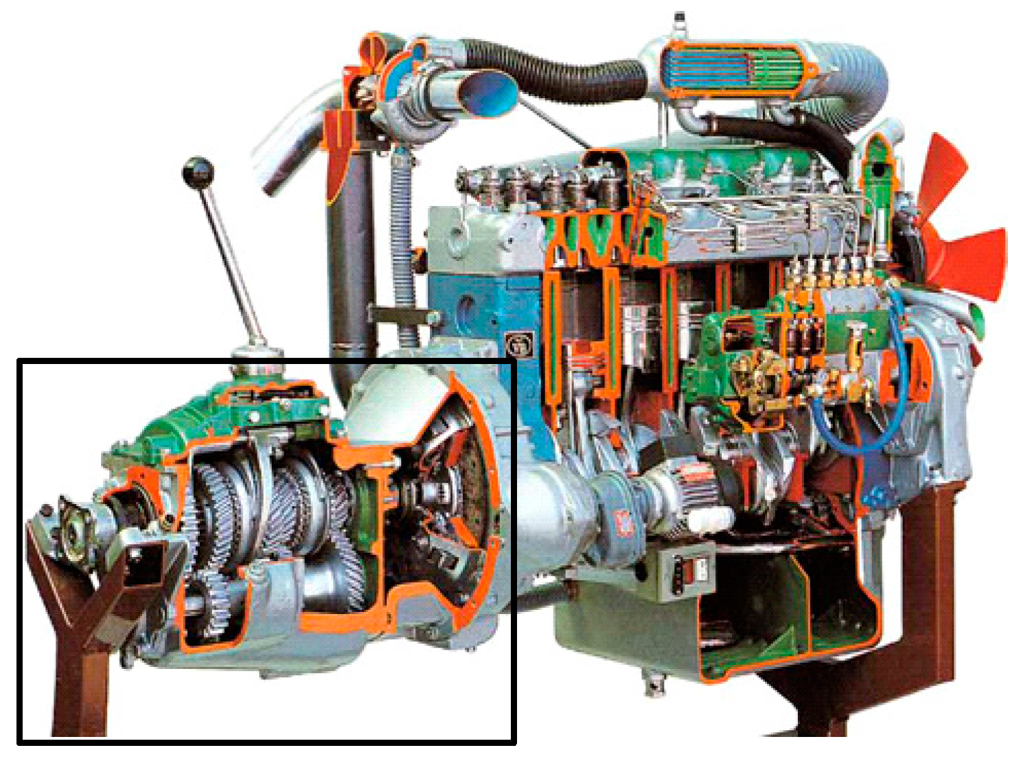
RUL of a diesel generator gearbox is studied by analyzing the vibration signals of a gearbox shell surface as
Figure 8 showed. Data comes from the High Stress Accelerated Life Test of a certain type of heavy high-speed vessel diesel manufactured by the China Shipbuilding Industry Corporation (CSIC), which is collected from the gearbox Monoblock’s accelerometers. The number of teeth of the drive pinion is 17, and the number of teeth of the driven bull gear is
75. The input shaft bearing has a pitch diameter of 60 mm, a rolling element diameter of 19.05 mm, and six steel balls; the output shaft bearing has a diameter of 95 mm, a rolling element diameter of 22.25 mm, and eight steel balls. The data were recorded every 5 or 10 min at a sampling rate of 20 KHz. Four sets of diesel generator gearbox data were recorded during the life-cycle degradation process in
Table 1.
GU1, GU2, GU3, and
GU4 all belong to the same type of component of the system, which are of similar working environments and operating conditions.
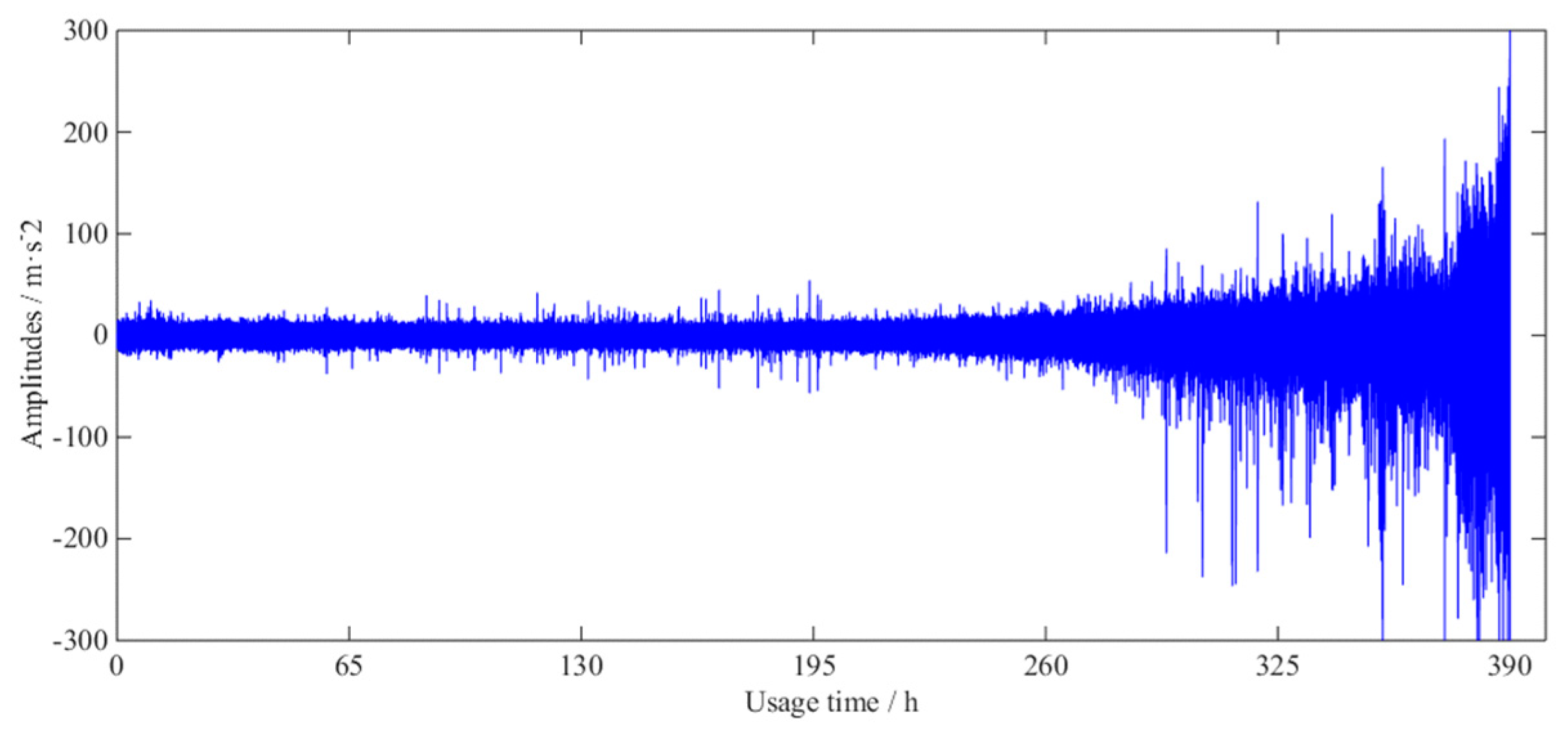
Figure 9 depicts the whole vibration signal in a gearbox lifecycle. The amplitude of the vibration signal increases gradually until the gear box fails to work properly.
3.1. Parameters System: Gearbox Performance Degradation Data
With the theory in
Section 2.1 and
Section 2.2, the evaluation result of 25 damage indicators is showed in
Table 2. According to the calculation result of Equation (7), the weights are
= 0.2,
= 0.5, and
= 0.3, respectively. According to the
Section 2.2, the first six damage indicators (
Fp9,
Fp13,
Fs4,
Fp3,
Fs2, and
Fp1) ranked from large to small according to the
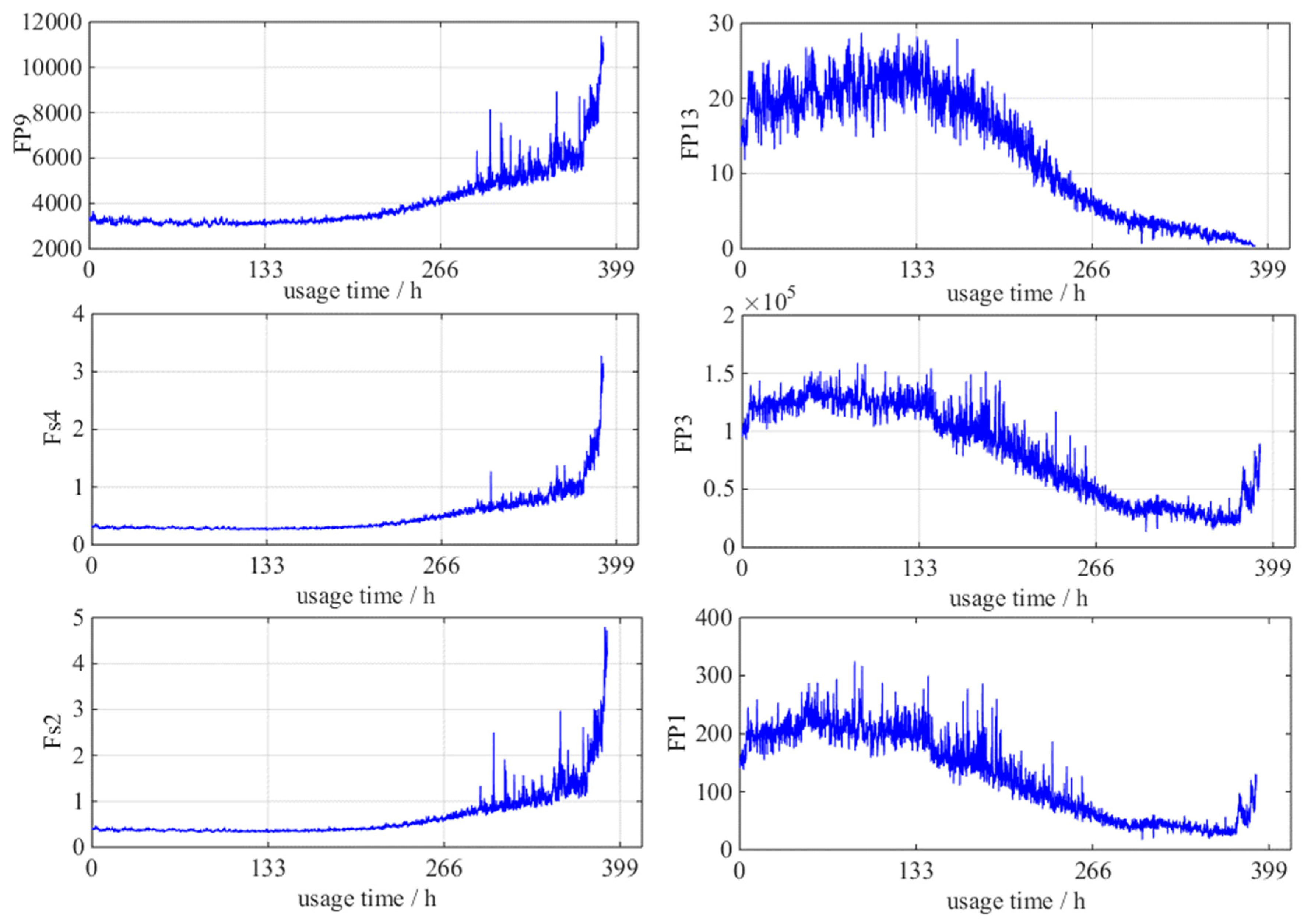
W value are selected to construct the performance damage indicator system of the diesel generator gearbox. They will be the input of two RUL estimation methods.
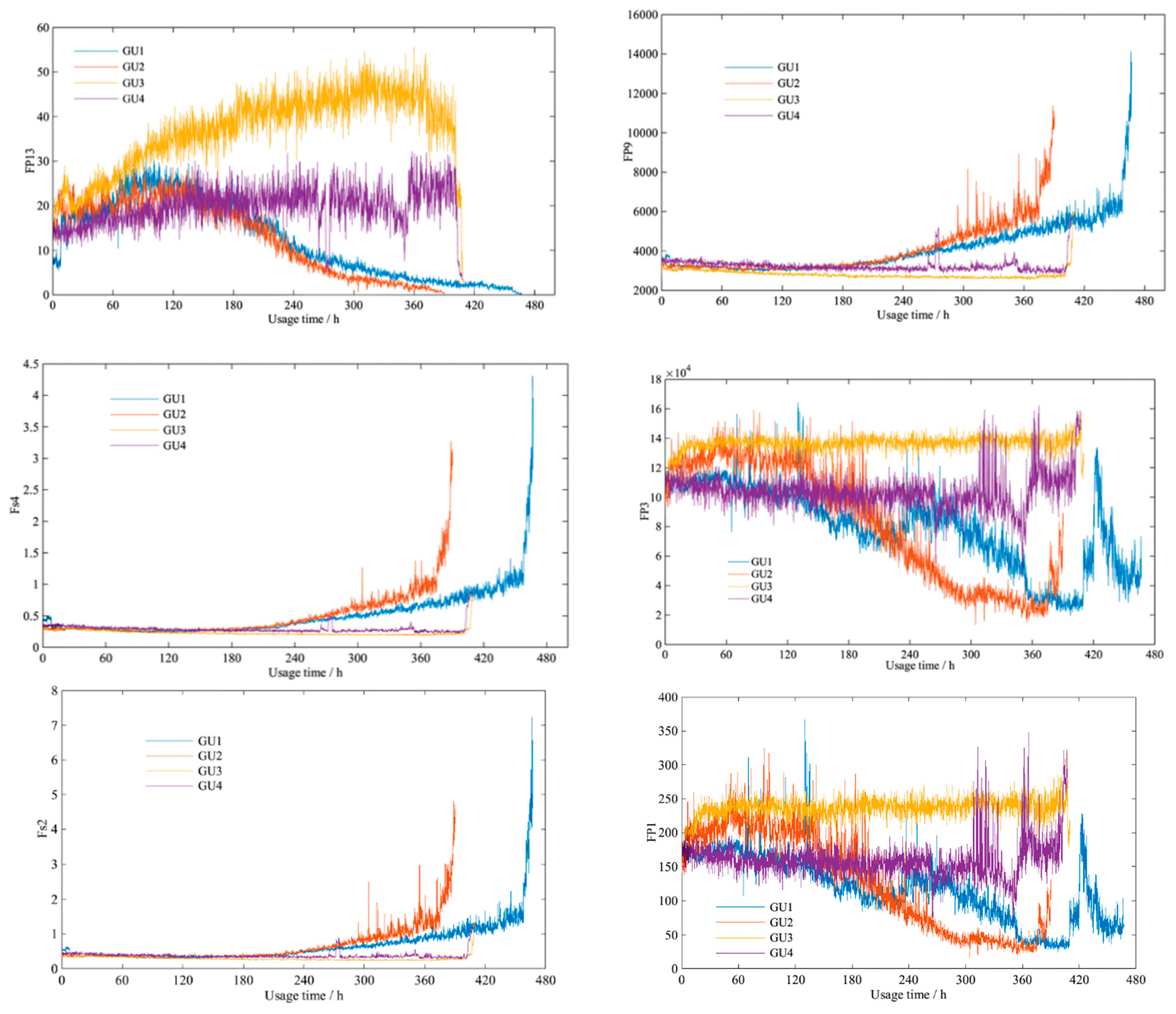
Figure 10 shows the life-cycle trajectories of
Fp9,
Fp13,
Fs4,
Fp3,
Fs2, and
Fp1.
After establishing the gearbox performance damage indicator system [
Fp9,
Fp13,
Fs4,
Fp3,
Fs2,
Fp1], the performance damage indicator data set of four samples (GU1 to GU4) is calculated.
Figure 11 indicates that the curves of the same performance damage indicator from different samples have similar states. This proves that the gearbox registers a similar degradation trajectory in line with the running state and environment, which provides strong practical evidence for the subsequent
RUL prediction based on multi-parameter and multi-sample similarity fusion. On the other hand, the different characters of
FP13, FP3, and
FP1 exactly reflect the different performance degradation trajectories of four samples. By selecting samples with different performance degradation, the verification of experience could be more convincing. In addition, in the aspect of the sample,
FP13, FP3, and
FP1 from a same sample have similar degradation trajectories, and the amplitude ranges are also so similar. This proves that these three parameters could actually reflect the performance degradation and should be selected for
RUL prediction.
Considering the running time and data features, this study sets Sample GU1 as the test sample and GU2, GU3, and GU4 as reference samples to prove the validity of multi-parameter and multi-sample similarity fusion.
3.2. RUL Prediction Results
(1) Results based on multi-parameter similarity fusion
This study unrolled the prediction of a diesel generator’s data starting from the point of 200 h, with the time window
D of 30. The details of
RUL prediction result based on multi-parameter similarity fusion with Euclidean distance/
DTWD are shown in
Table A3 and
Table A4 of
Appendix B.
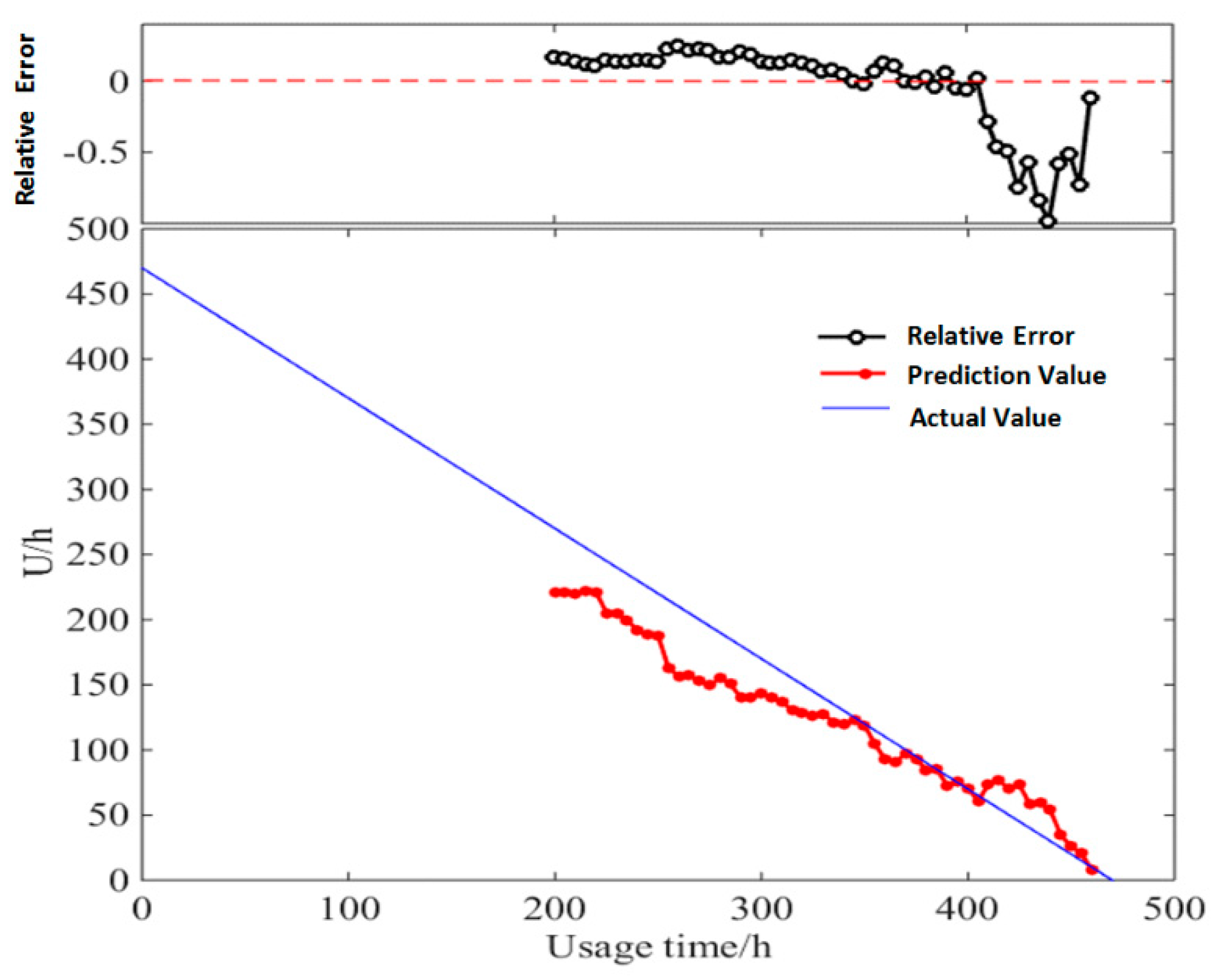
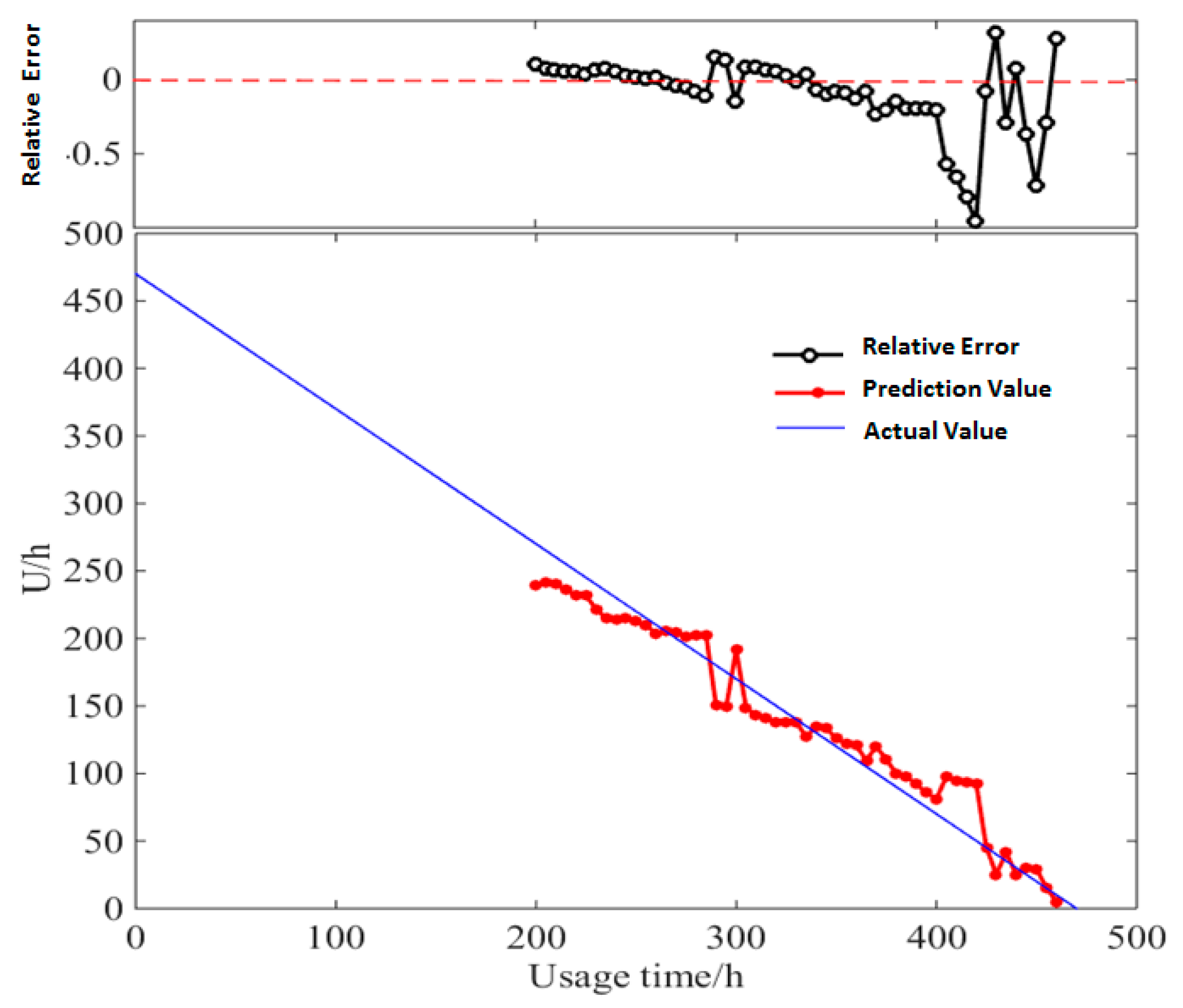
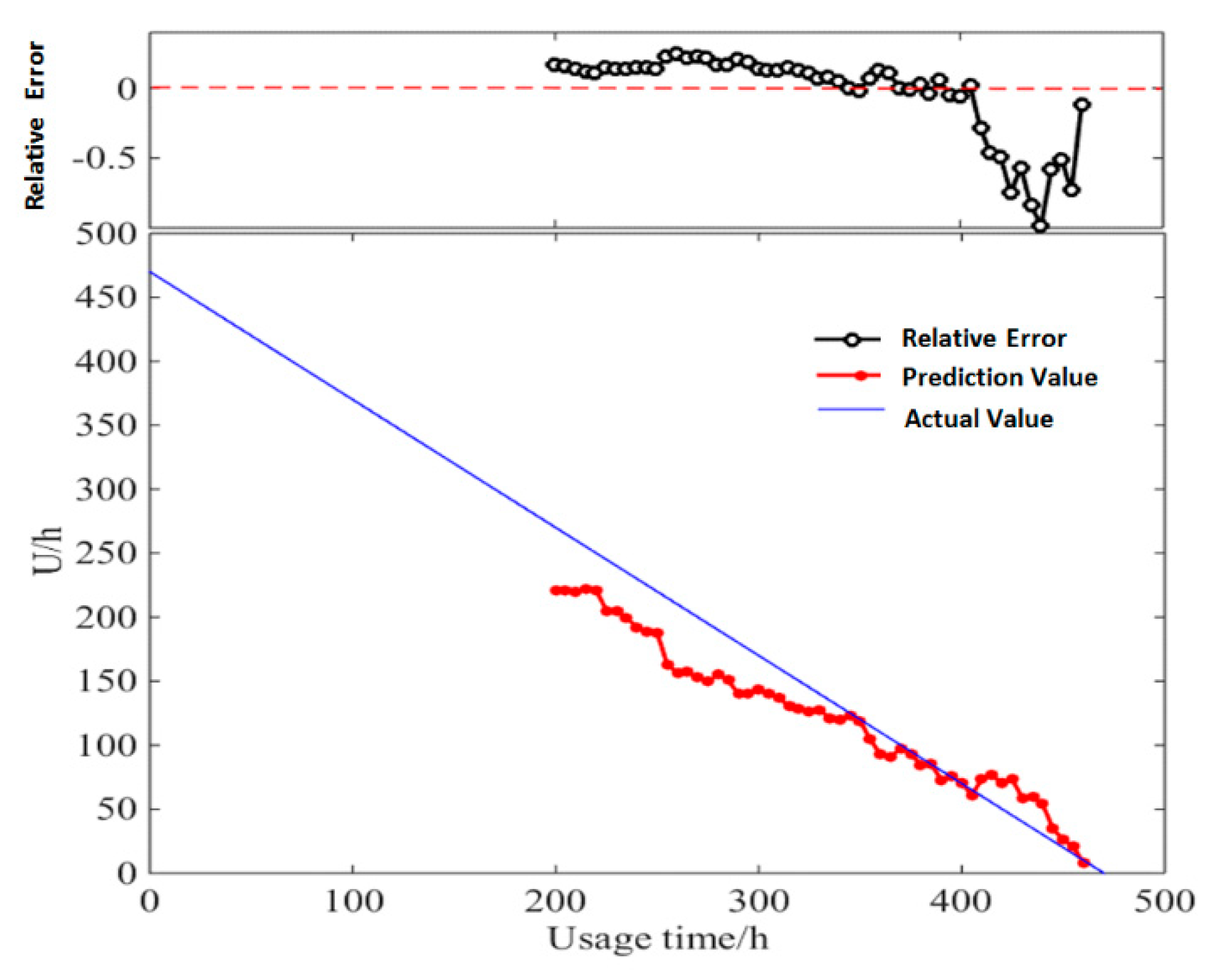
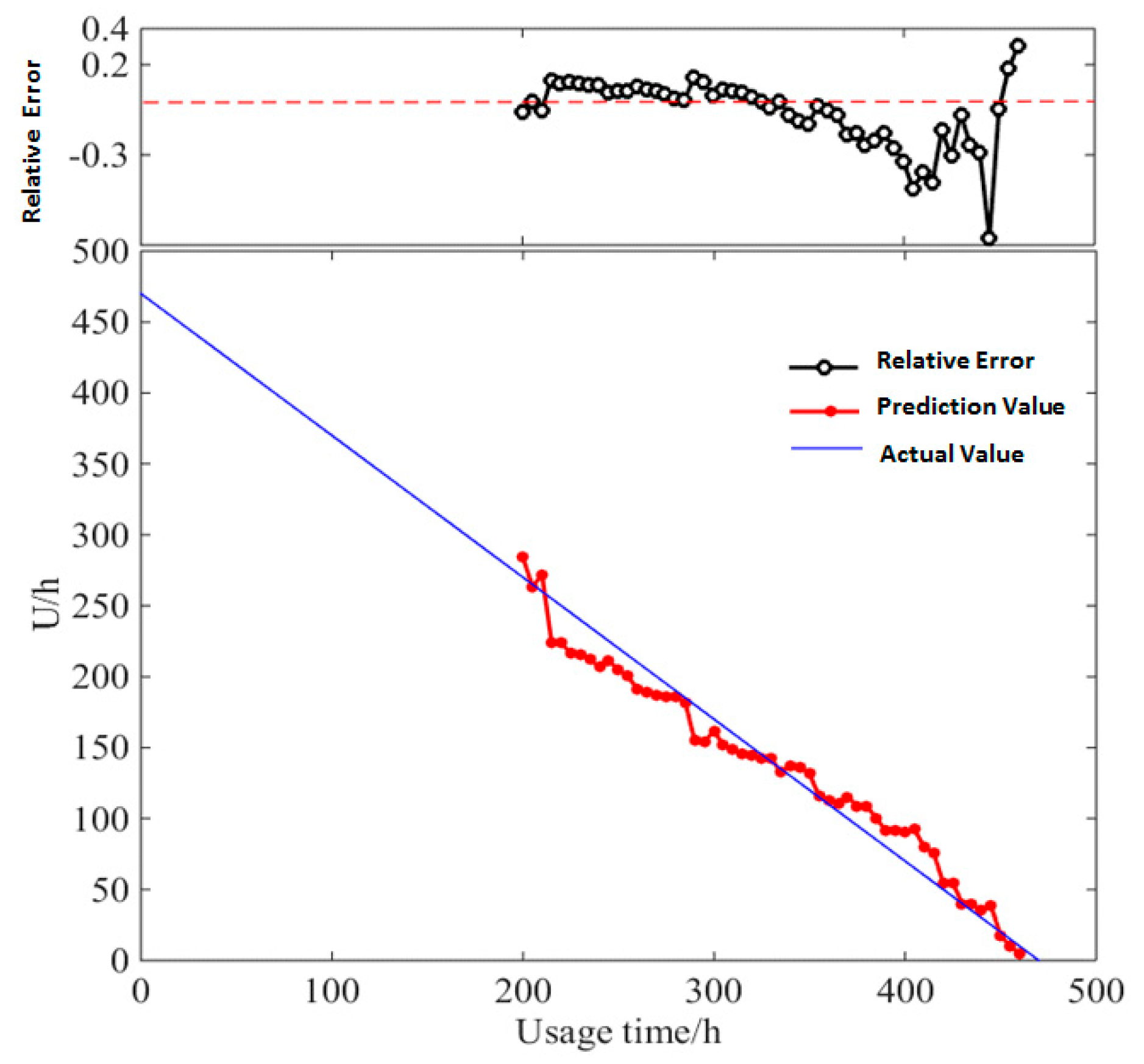
Figure 12 and
Figure 13 show the relative error between the actual values and predicted values of
RUL.
In RUL prediction based on multi-parameter similarity fusion with DTWD, the relative error between the predicted values and the actual values ranges from −0.88% to −95.82%. Except for very few points with large errors, the relative errors of most of the predicted values are below 30%, which could obtain more accurate values than traditional Euclidean distance.
(2) Result based on multi-sample similarity fusion
The
RUL estimation values based on multi-sample similarity fusion during the life-cycle degradation process are shown in
Table A5 and
Table A6 of
Appendix B.
Figure 14 and
Figure 15 show the relative error between the actual values of
RUL and the predicted values with Euclidean distance /
DTWD.
With RUL prediction based on multi-sample similarity fusion, the relative error between the predicted values and the actual values ranges from −0.35% to −76%. Except for very few points with large errors, the overall relative error is controlled below 30%, which has a better prediction accuracy than the RUL prediction result based on multi-parameter similarity fusion.
3.3. Comparative Analysis with Single-Parameter RUL Prediction
Unlike methods of single-parameter similarity fusion, the method of multi-parameter similarity fusion generates a combination of results predicted by multiple parameters. In order to prove the validity and rationality of the model, a performance degradation curve is established upon each and every one of the reference samples’ parameters. The calculation adopts that of the single-parameter similarity prediction method and the weight value calculation process of different reference samples is the same as above. The test data set contains six performance damage indicators of Sample GU1: Fp9, Fp13, Fs4, Fp3, Fs2, and Fp1. They are compared to parameters Fp9, Fp13, Fs4, Fp3, Fs2, and Fp1 of Sample GU2, GU3, and GU4 to determine the RUL.
In this study, Principal Component Analysis (
PCA) technology is used to integrate elements of the performance degradation index system [
30]. The first principal component
PCA-1 and the second principal component
PCA-2 were extracted respectively to conduct
RUL prediction through the single-parameter life
RUL prediction method [
31]. This paper takes the life cycle data set of Sample GU1 as an example. Through
PCA of its six performance damage indicators, we get the
KMO of 0.748, higher than 0.5, indicating that the six parameters are suitable for dimensionality reduction processing.
The curve of the first-order principal component and second-order principal component of the performance damage indicator system of Sample GU1’s life cycle data is shown in
Figure 16.
The single-parameter
RUL prediction results of the first-order performance principal component
PCA-1 and the second-order principal component
PCA-2 are shown in
Table 3.
It can be seen from the table that there are significant differences in the prediction effects of the six parameters in the diesel generator gearbox performance degradation index system. The prediction accuracy of Fp13 and Fs4 is higher than the rest, whereas the prediction of all the six first-order principal components of PCA-1 is more accurate than that of a single-parameter. The single-parameter similarity RUL prediction registers a poorer performance. In summary, the multi-parameter fusion-based RUL prediction method proposed in this study has certain advantages and effectiveness.
3.4. Comparative Analysis with AI-Based RUL Method: MSVM
Research on
RUL prediction based on artificial intelligence has also been developed, such as Bayesian methods, which are deep learning methods. This paper uses the multivariable support vector machine (
MSVM) for comparative analysis.
MSVM fully considers the interaction and constraints between multiple variables, and realizes the maximum mining of potential information for small sample data. According to
Section 3.1,
Fp9, Fp13, Fs4, Fp3, Fs2, and
Fp1 are selected as the input of
MSVM, and a regression function is constructed:
w and
b can be obtained by solving the optimum solution of the following equation:
C is a penalty factor,
are relaxation factors, and
is an unsensitive factor. When the data set shows a nonlinear relationship, a kernel function is introduced into the
SVM operation to map the original data into the high-dimensional feature space. The Radial Basis Function (
RBF) and Poly kernel function are as follows:
P is the index of
RBF. The Lagrangian function is introduced to transform the optimization problem into a convex quadratic programming problem.
,
are Lagrangian multipliers.
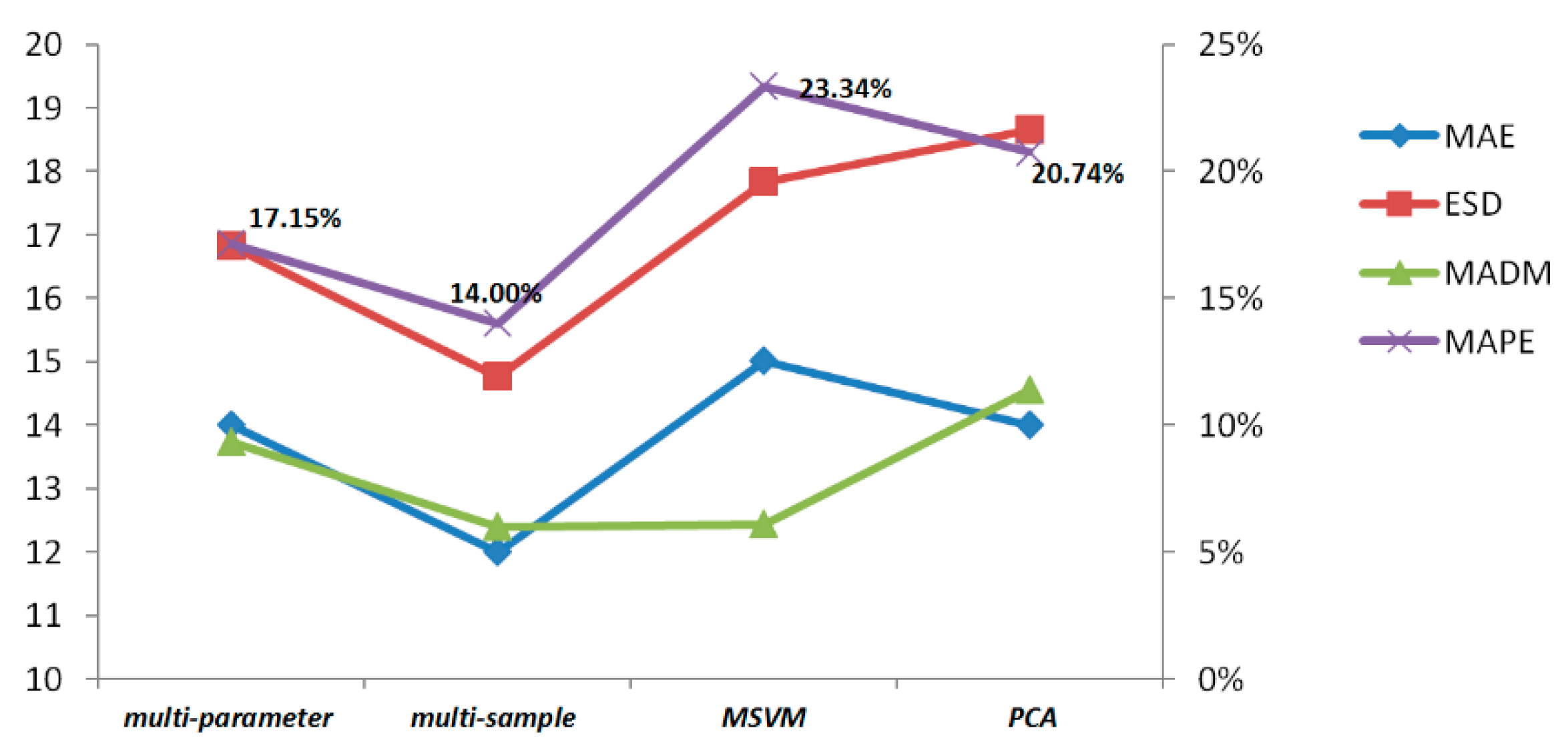
The calculation results of the comparative analysis are shown in
Table 4.
Table 4 indicates that the prediction accuracy of multi-sample similarity fusion is higher than multi-parameter similarity fusion concerning the prediction’s average relative error, and the two methods’
MAPE are both lower than
MSVM, validating the effectiveness of the proposed method compared with the
AI-based method. In addition, the proposed
DTWD-based algorithm performs better than the traditional Euclidean distance.
In parameter similarity fusion, RUL values predicted by the same performance damage indicators are integrated to calculate the RUL of the test sample; while in sample similarity fusion, the RUL values of samples are integrated on the basis of performance damage indicators carried by each sample.
Multi-parameter and multi-sample methods are similar in calculation, but differ in some respects. Multi-parameter similarity fusion depends more on parameters’ feedback on the performance degradation process, while multi-sample similarity fusion relies on the sample data that is similar to the life-cycle trajectory in the gearbox running process. The more similar the test samples are with reference samples in terms of operating methods, conditions, and load environments, the larger the weight value that can be obtained, and the closer the
RUL prediction value is to the actual value. Experimental results of the comparison are shown in
Figure 17.
3.5. Limitations and Future Work
This paper proposes an RUL prediction model based on multi-parameter and multi-sample fusion, and has verified its effectiveness through analyzing a certain type of heavy high-speed diesel generator manufactured by an affiliate of CSIC. The results show that the proposed method is superior to previous studies in terms of the prediction accuracy. However, there are still some limitations in several respects. First, this paper verifies the proposed model with the diesel generator gearbox as an example, but further efforts should be devoted to testing broader gearbox equipment and even the mechanical rotating equipment. Second, this study does not classify types of malfunction at the termination and identify the degradation trend at different stages. Future researches can focus more on RUL under different malfunctions, grouping and decomposing the performance degradation process to identify test samples’ running stages, and refining the RUL prediction problems and models. Third, the research is conducted on the vibration signal of the diesel generator gearbox. To develop a more comprehensive RUL prediction method, future research should incorporate more data sources, such as performance parameters and environmental parameters.
