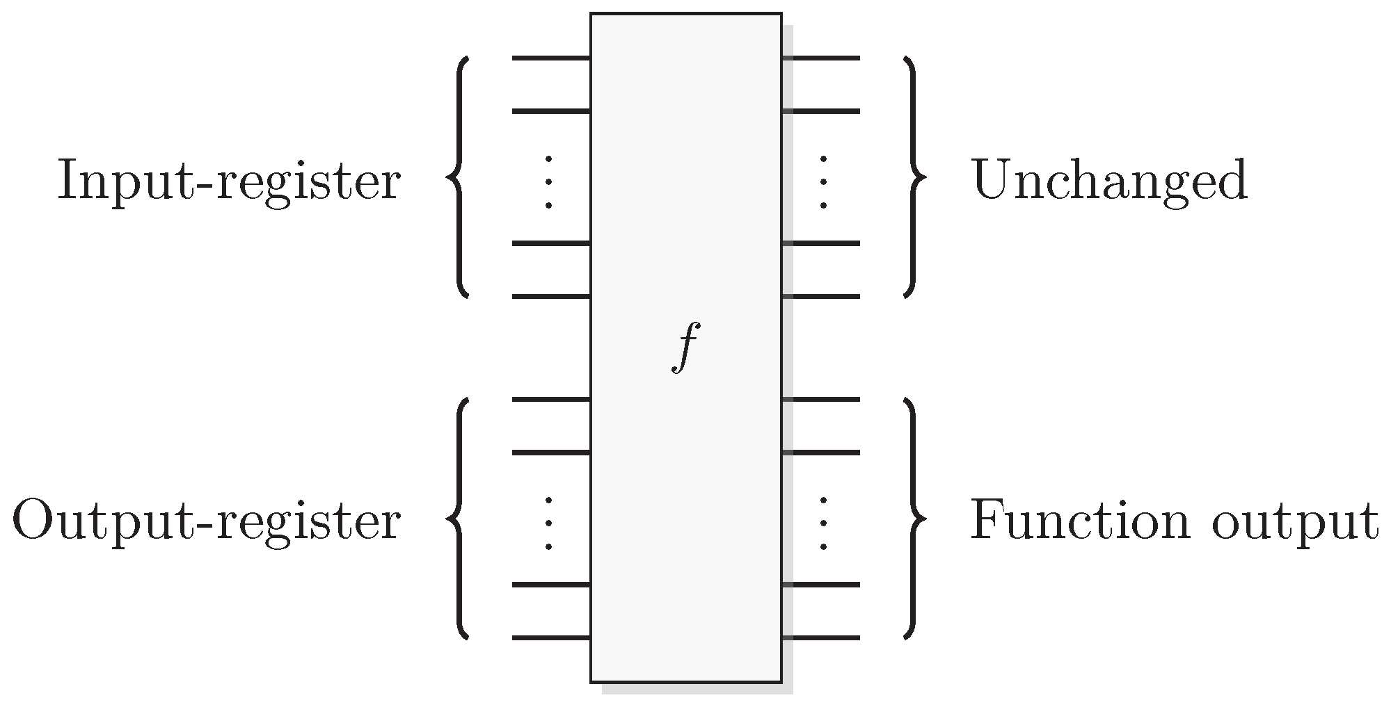
Figure 1.
A classical reversible logical function construction for a function f.
Figure 1.
A classical reversible logical function construction for a function f.
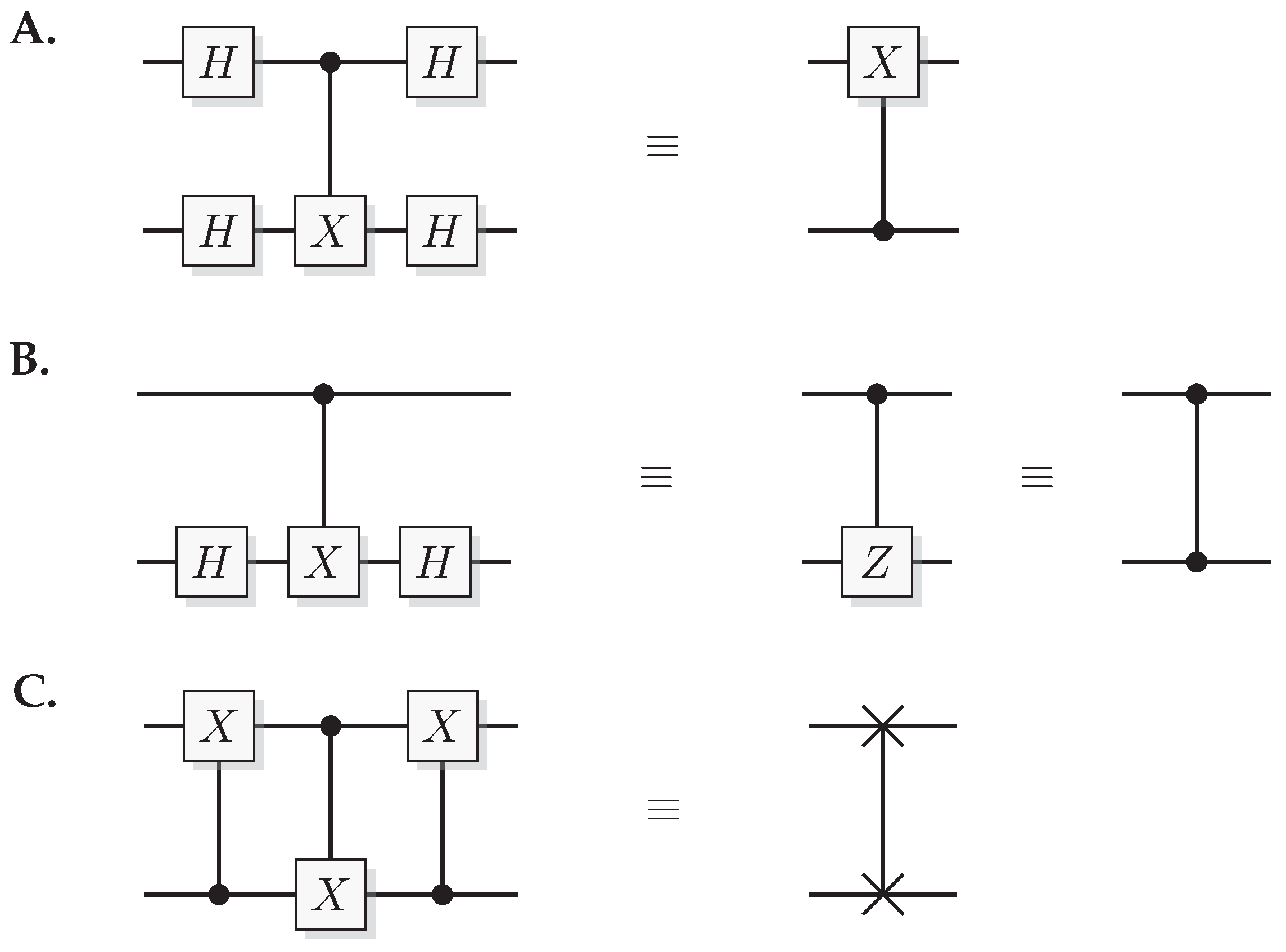
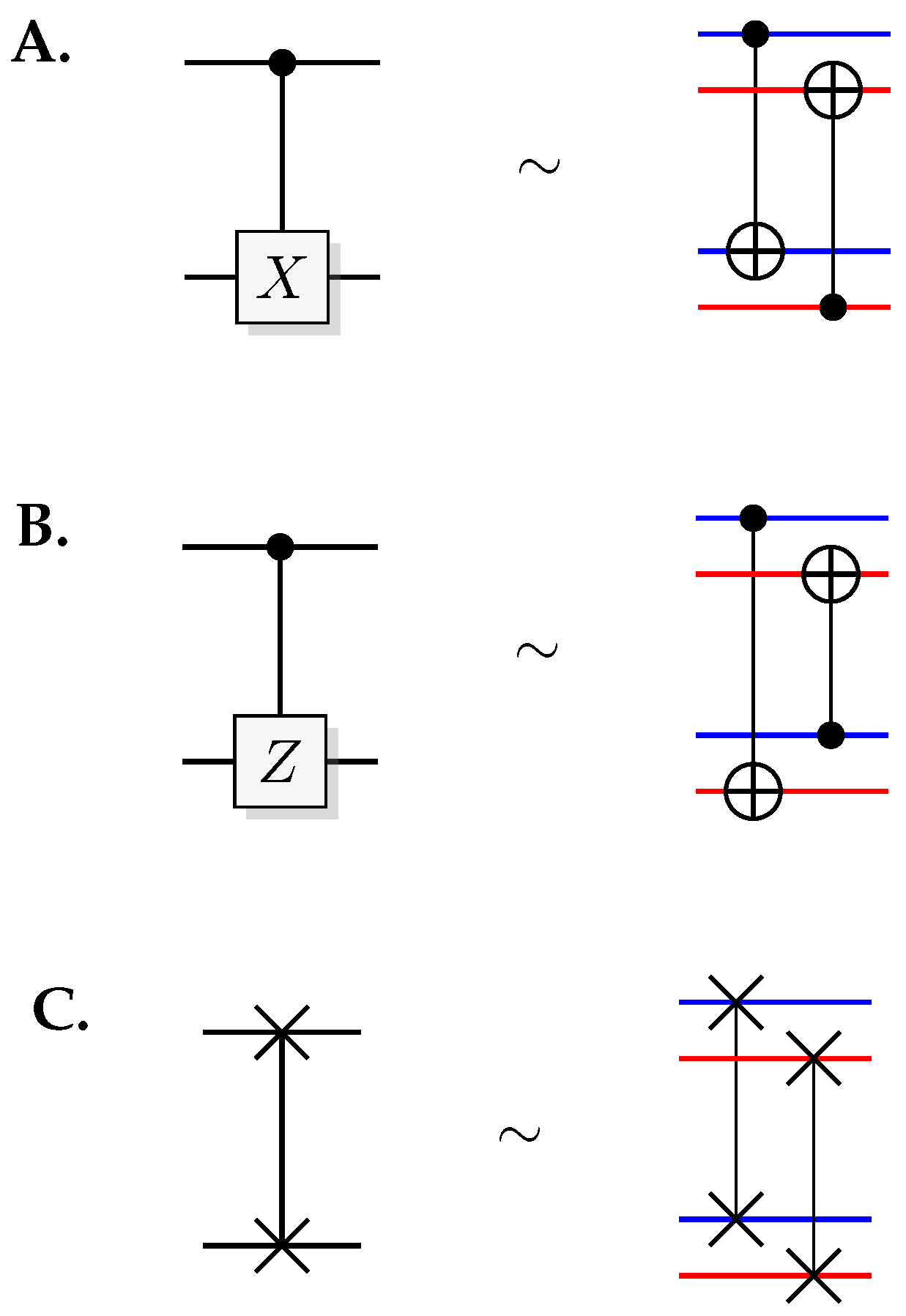
Figure 2.
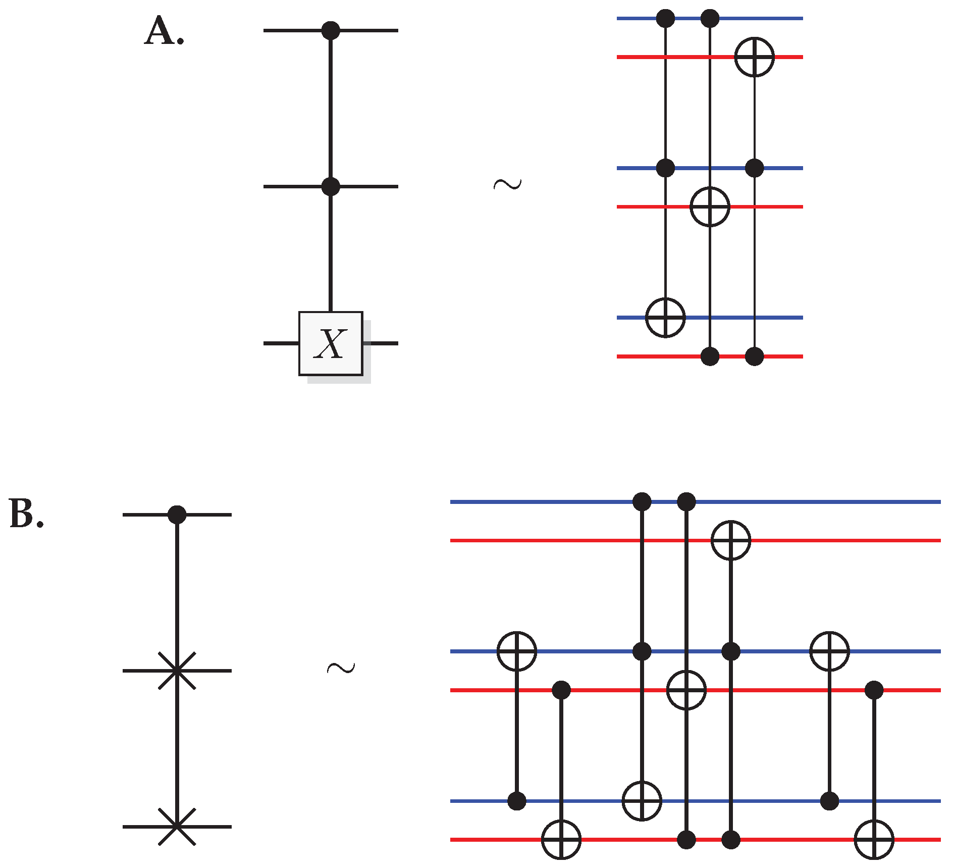
Identities for two-qubit quantum gates. (A) The effect of a quantum CNOT in the Hadamard basis. (B) relation between CNOT and CZ. (C) construction of a SWAP gate from three CNOT gates.
Figure 2.
Identities for two-qubit quantum gates. (A) The effect of a quantum CNOT in the Hadamard basis. (B) relation between CNOT and CZ. (C) construction of a SWAP gate from three CNOT gates.
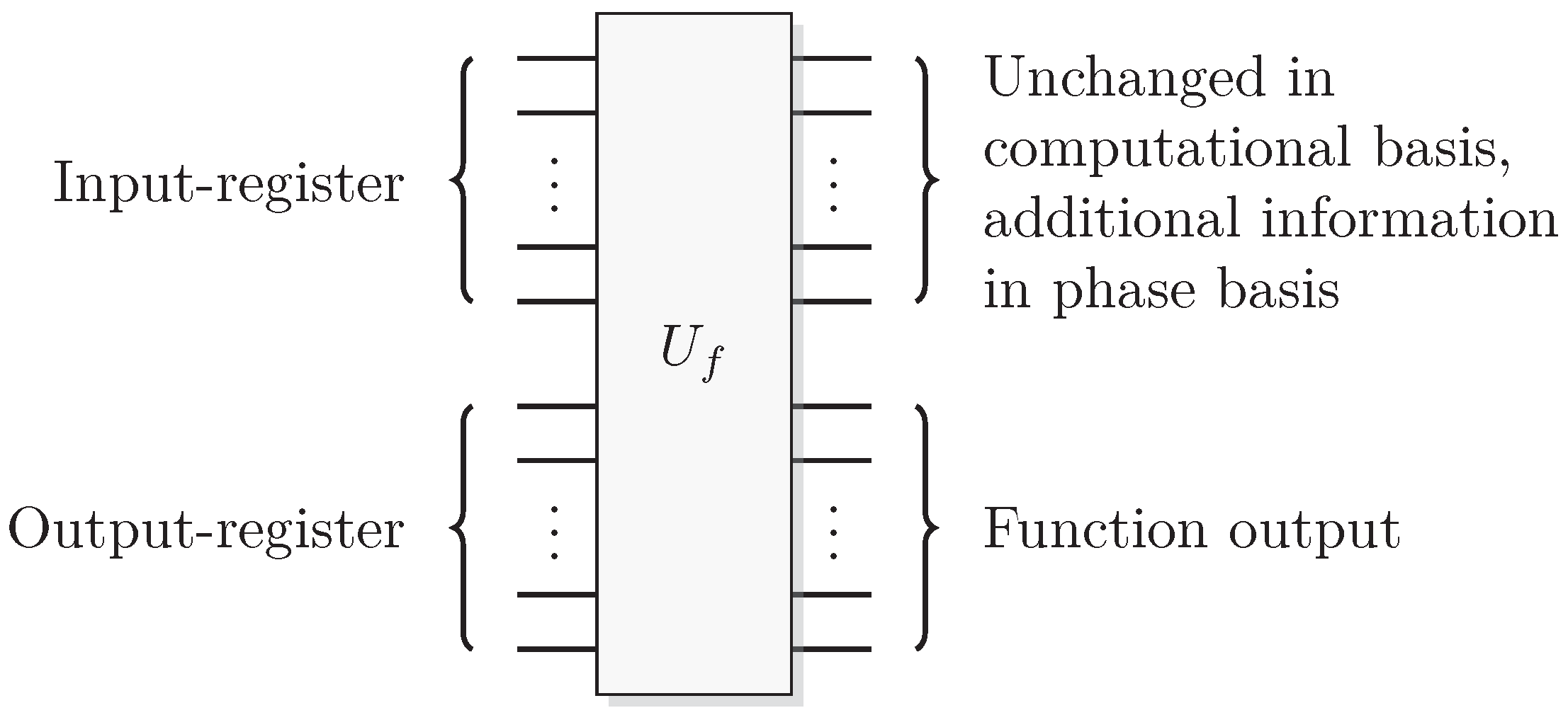
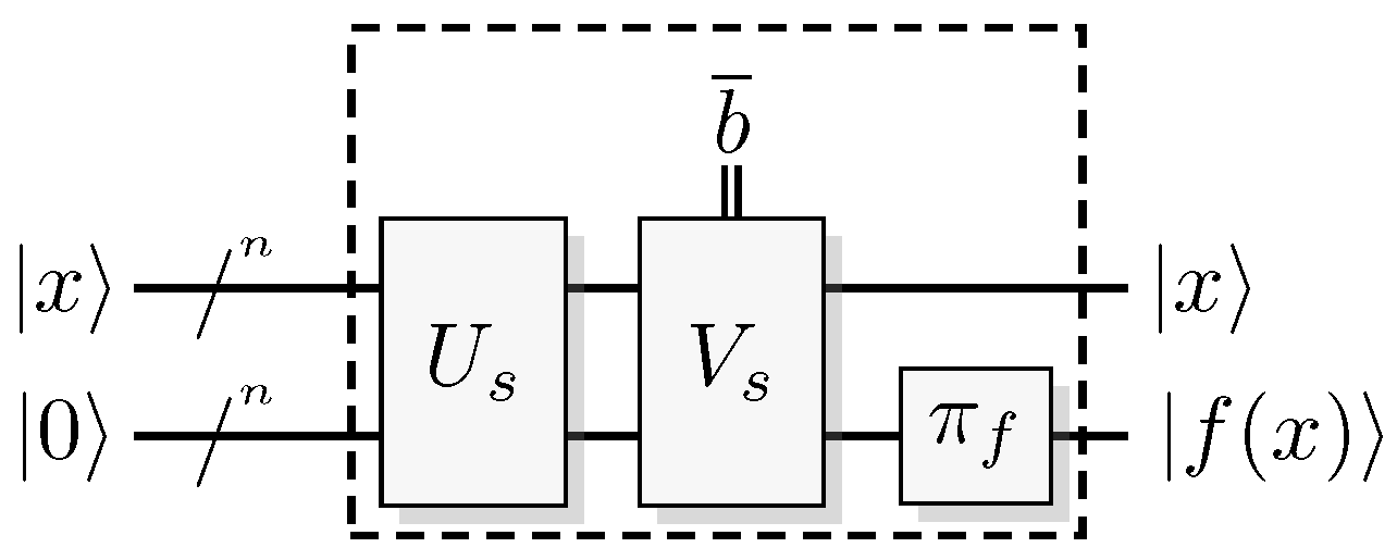
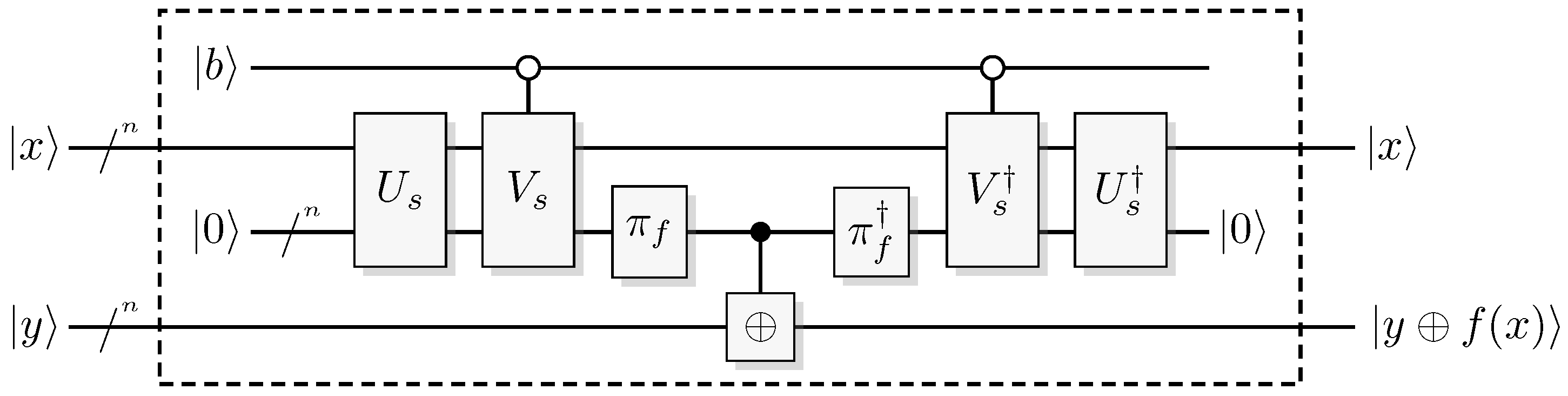
Figure 3.
A reversible logical function. In the quantum case we can choose to retrieve function output or some additional information from the output of the query register.
Figure 3.
A reversible logical function. In the quantum case we can choose to retrieve function output or some additional information from the output of the query register.
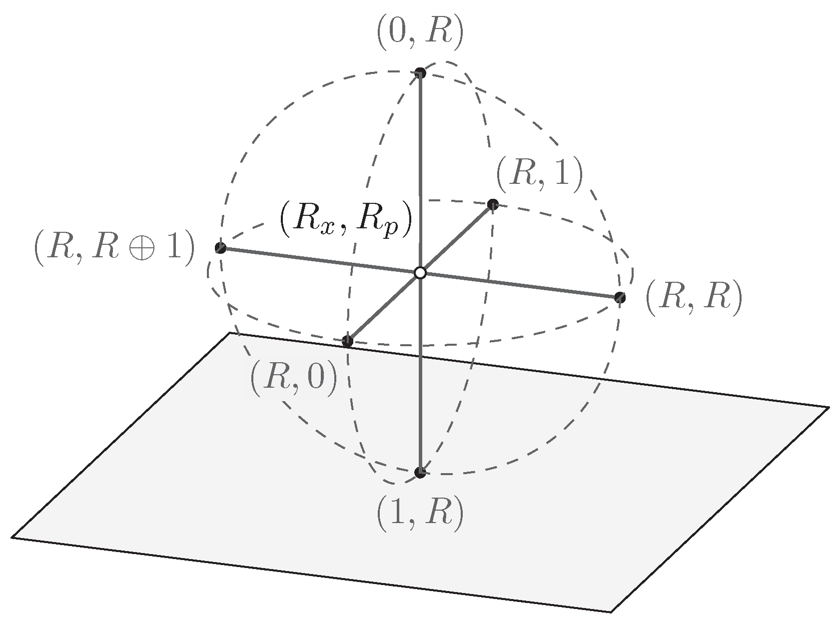
Figure 4.
Geometric representation of the seven states of an elementary QSL system and their position relative to the Bloch sphere.
Figure 4.
Geometric representation of the seven states of an elementary QSL system and their position relative to the Bloch sphere.
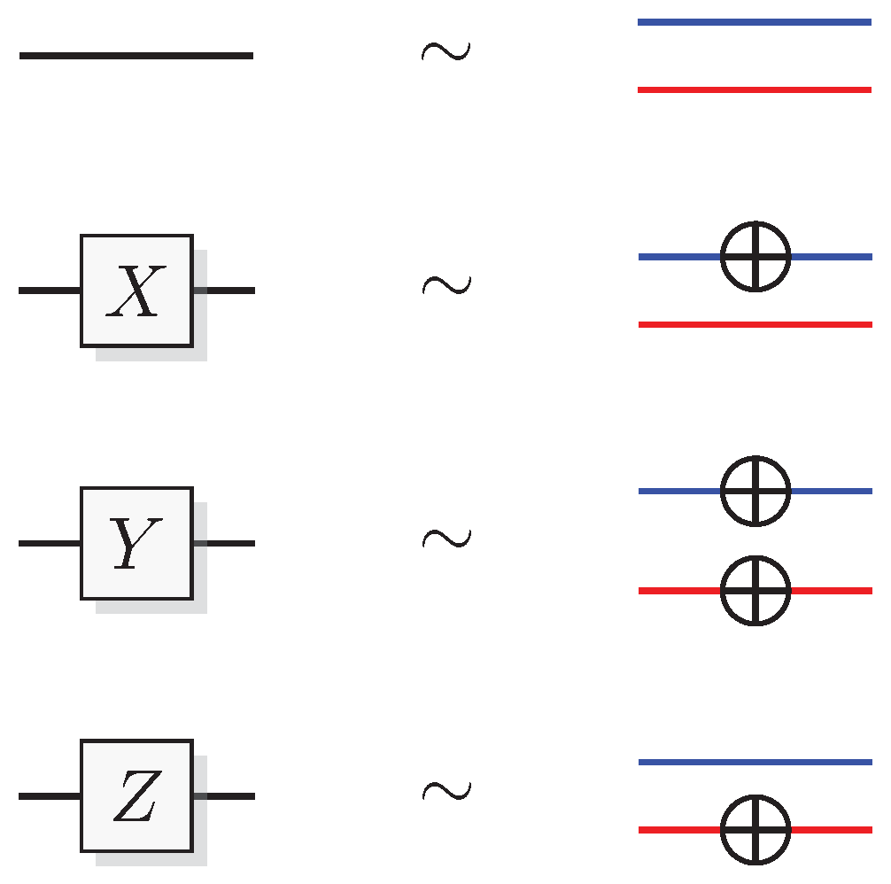
Figure 5.
Graphical representation of the simulation of the Pauli gates and Z. Blue line segments represent the computational bit and red represents the phase bit.
Figure 5.
Graphical representation of the simulation of the Pauli gates and Z. Blue line segments represent the computational bit and red represents the phase bit.
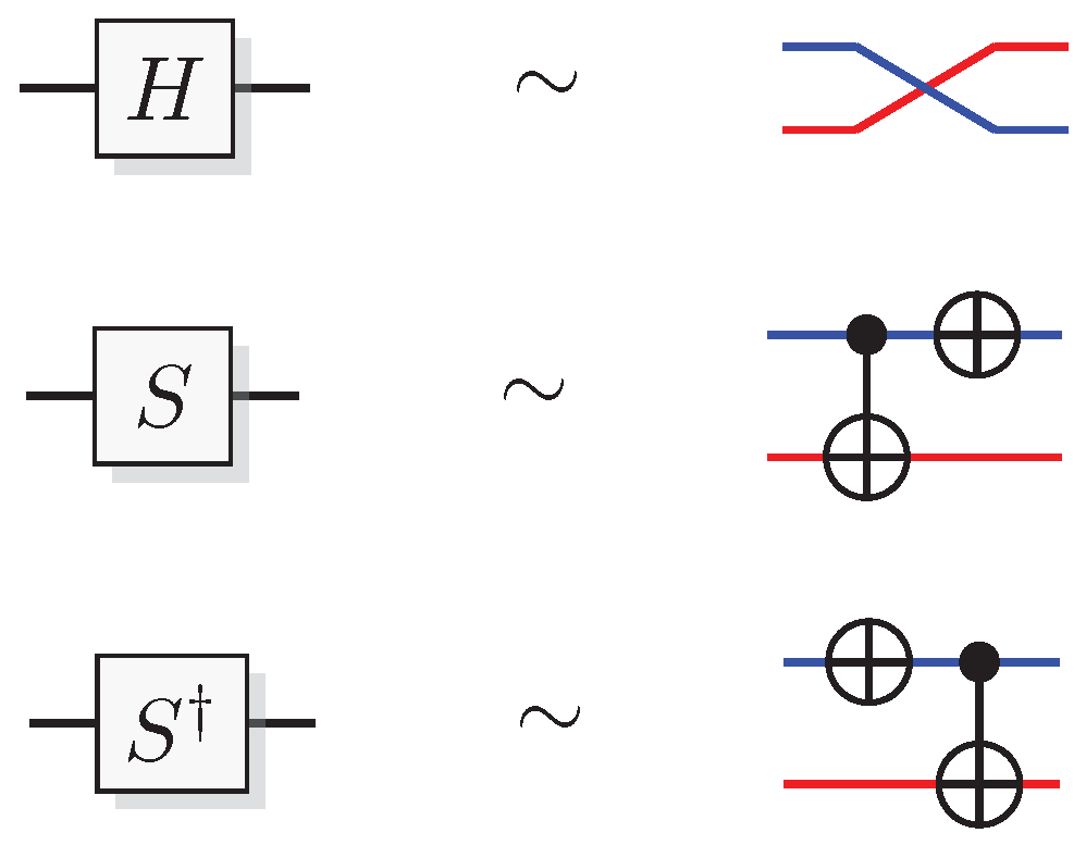
Figure 6.
Graphical representation for the simulation of Hadamard, S, and gates.
Figure 6.
Graphical representation for the simulation of Hadamard, S, and gates.
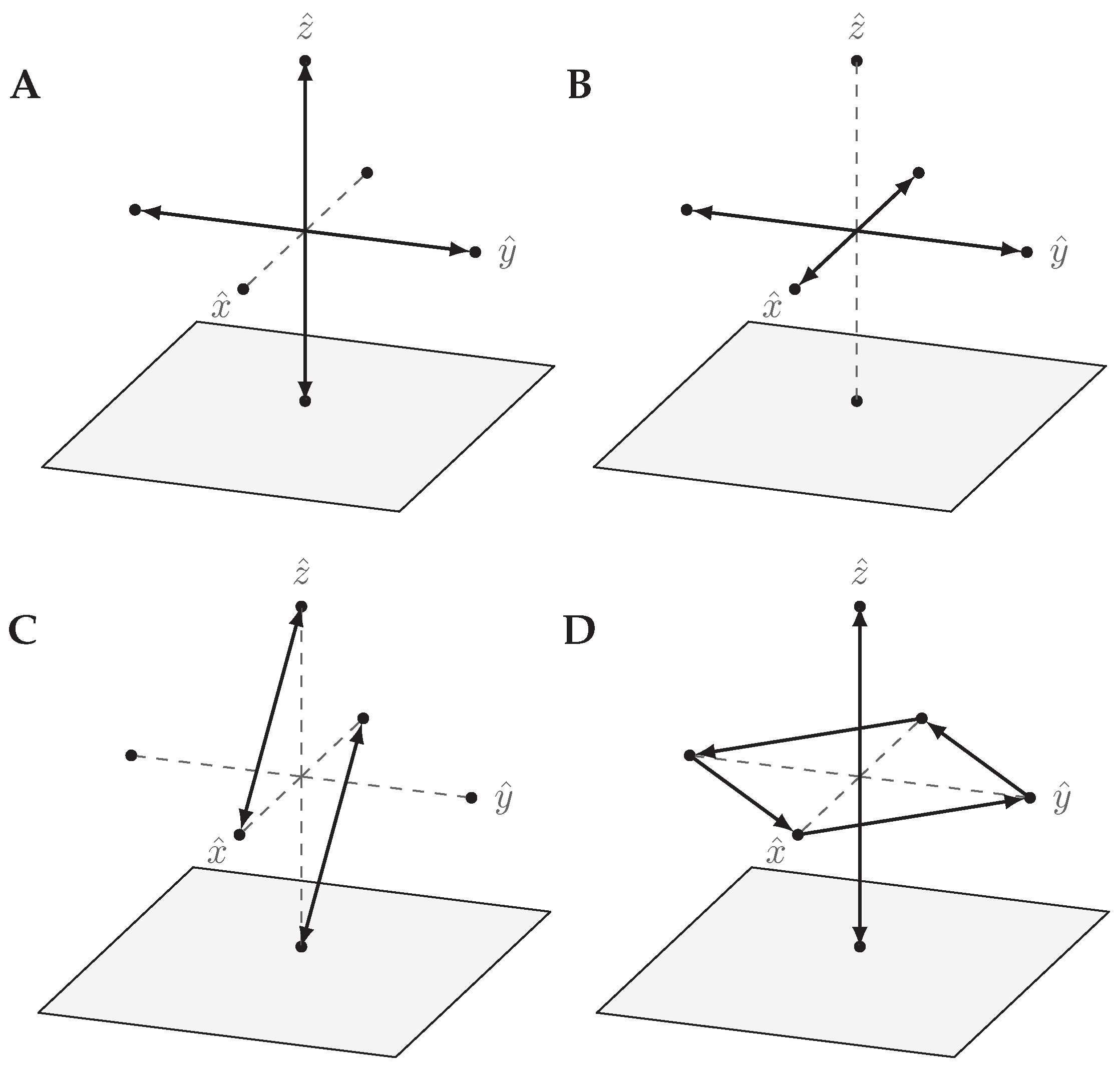
Figure 7.
Effect of the transformations on the six QSL states in the Bloch representation. (A–D) shows the , , , and gates, respectively.
Figure 7.
Effect of the transformations on the six QSL states in the Bloch representation. (A–D) shows the , , , and gates, respectively.
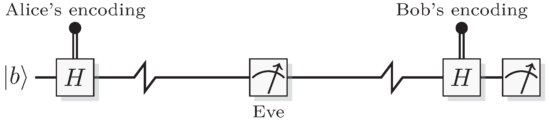
Figure 8.
The BB84 protocol with an eavesdropper present.
Figure 8.
The BB84 protocol with an eavesdropper present.
Figure 9.
Graphical representation of the QSL analogue of two-qubit quantum gates. (
A)
CNOT, (
B) controlled-
Z, and (
C)
SWAP, all constructed to uphold the identities in
Figure 2.
Figure 9.
Graphical representation of the QSL analogue of two-qubit quantum gates. (
A)
CNOT, (
B) controlled-
Z, and (
C)
SWAP, all constructed to uphold the identities in
Figure 2.
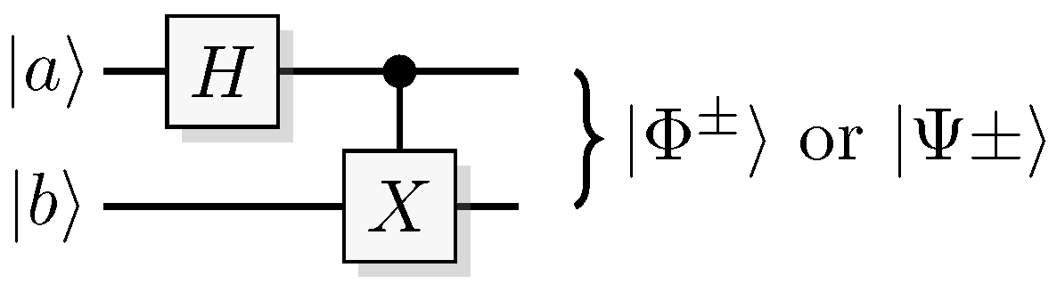
Figure 10.
Circuit for generating the four Bell states.
Figure 10.
Circuit for generating the four Bell states.
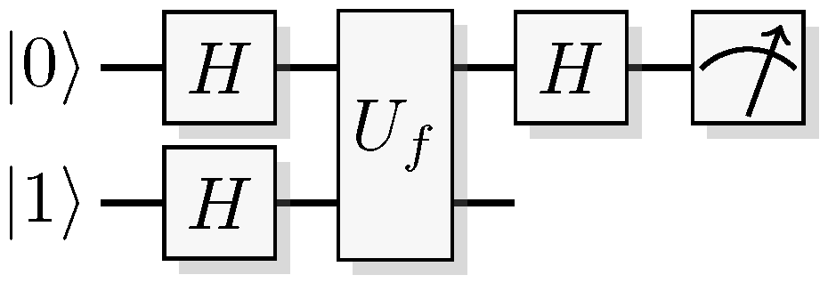
Figure 11.
Circuit for the Deutsch algorithm used to illustrate interference.
Figure 11.
Circuit for the Deutsch algorithm used to illustrate interference.
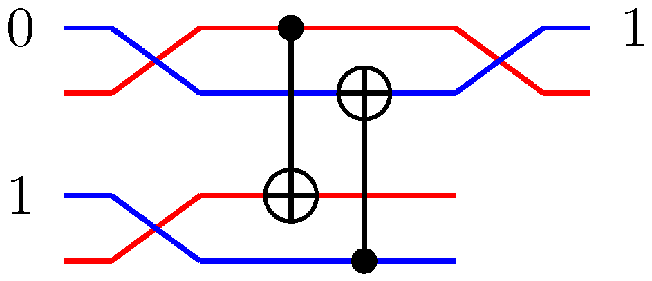
Figure 12.
Example of QSL simulating interference in Deutsch algorithm when .
Figure 12.
Example of QSL simulating interference in Deutsch algorithm when .
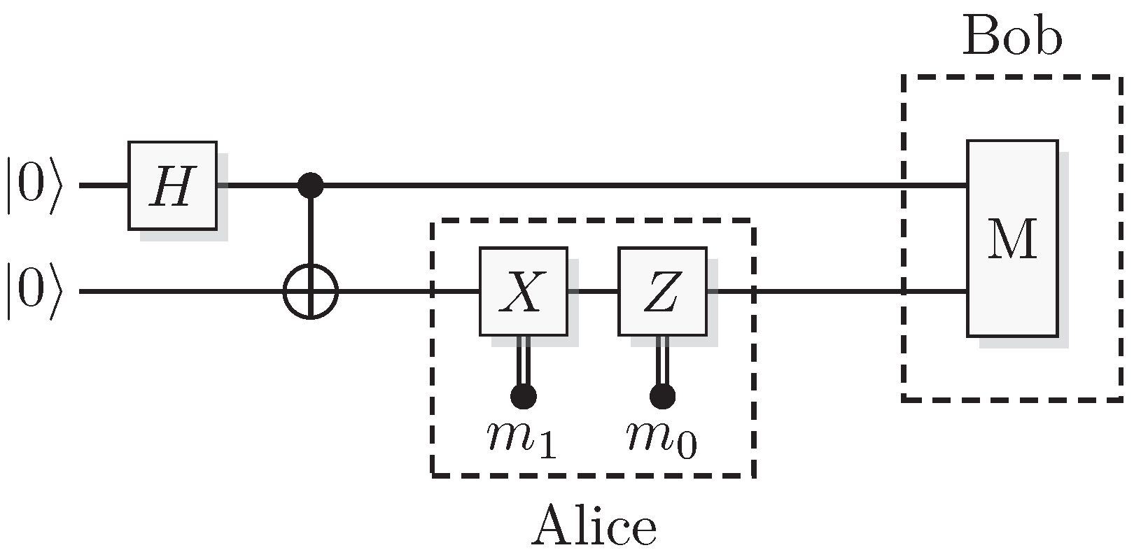
Figure 13.
Protocol for superdense coding. Alice can convey two bits of information and to Bob by only interacting with one qubit of a correlated pair.
Figure 13.
Protocol for superdense coding. Alice can convey two bits of information and to Bob by only interacting with one qubit of a correlated pair.
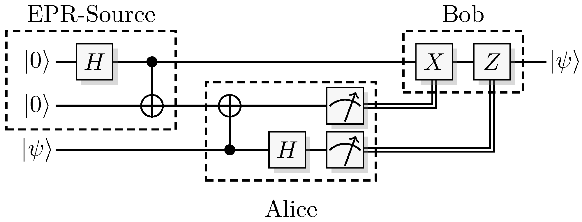
Figure 14.
The teleportation protocol.
Figure 14.
The teleportation protocol.
Figure 15.
QSL construction of the Toffoli gate (
A) and Fredkin (
B), constructed to uphold the identities in
Figure 16.
Figure 15.
QSL construction of the Toffoli gate (
A) and Fredkin (
B), constructed to uphold the identities in
Figure 16.
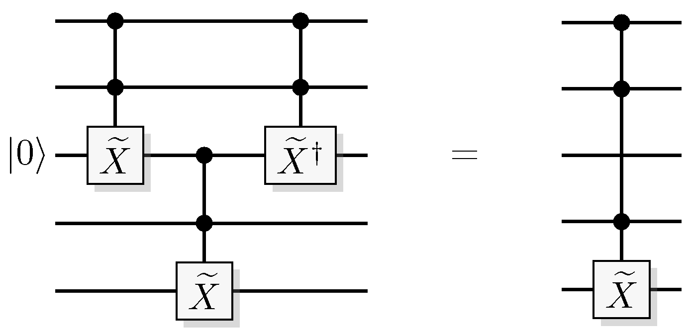
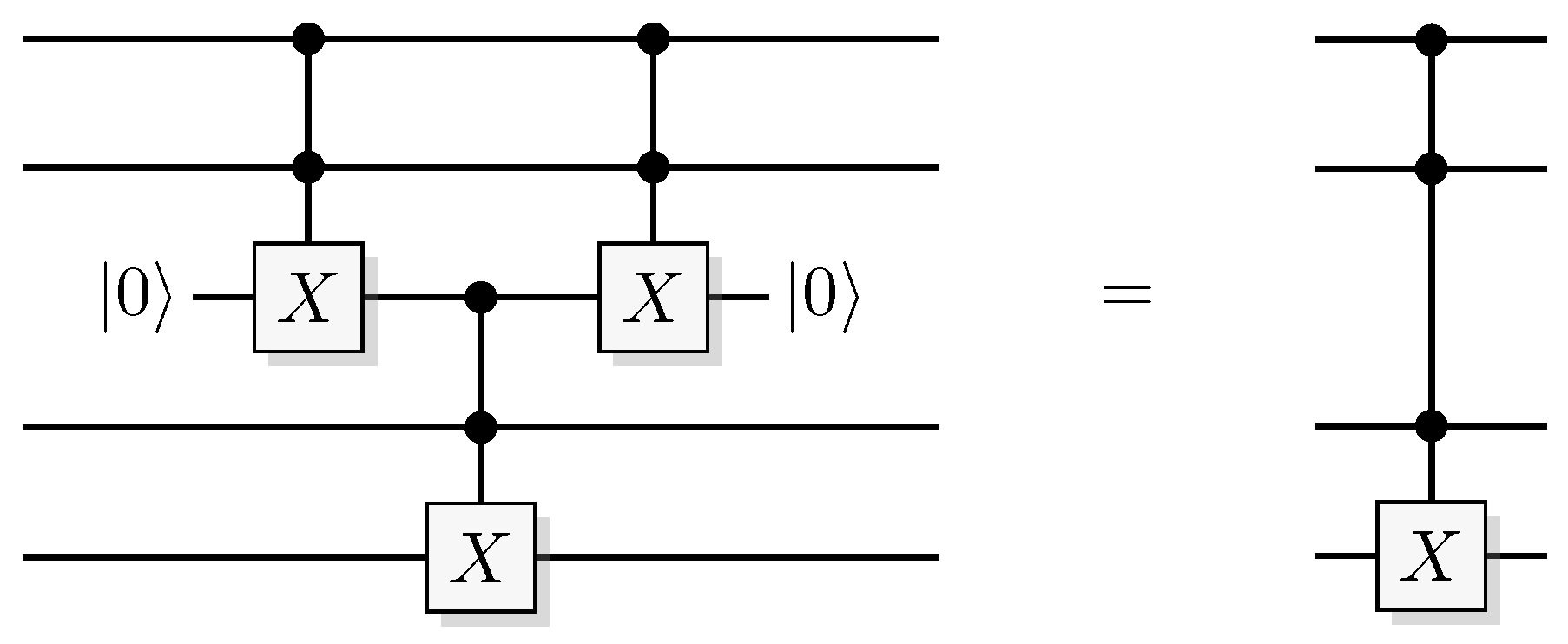
Figure 16.
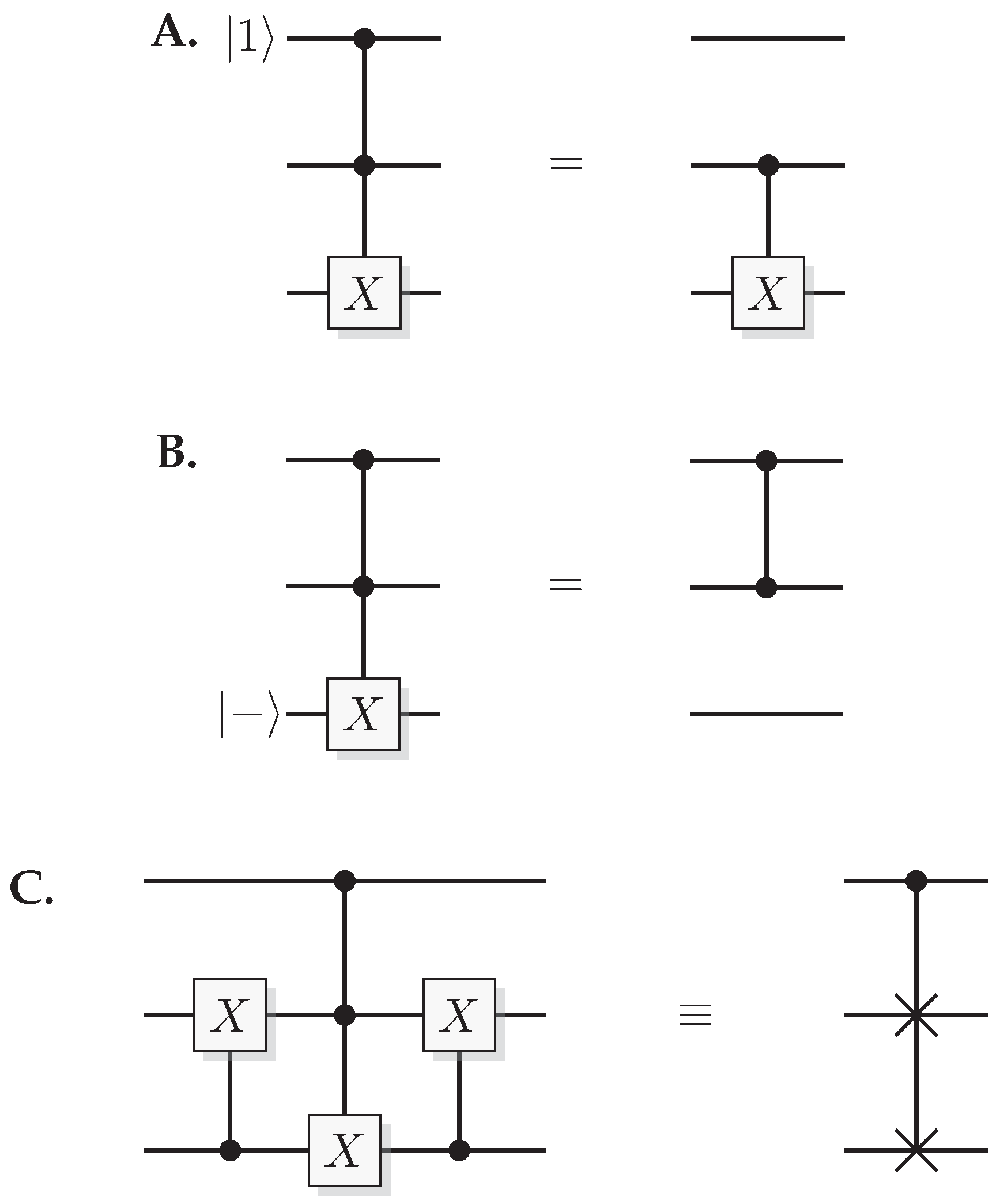
Quantum gate identities. (A) Toffoli gate with one of the controlling qubits initiated in results in a CNOT over the other two qubits. (B) Toffoli gate with the target qubit initiated in results in a over the control qubits. (C) Identity connecting the Toffoli and Fredkin gate.
Figure 16.
Quantum gate identities. (A) Toffoli gate with one of the controlling qubits initiated in results in a CNOT over the other two qubits. (B) Toffoli gate with the target qubit initiated in results in a over the control qubits. (C) Identity connecting the Toffoli and Fredkin gate.
Figure 17.
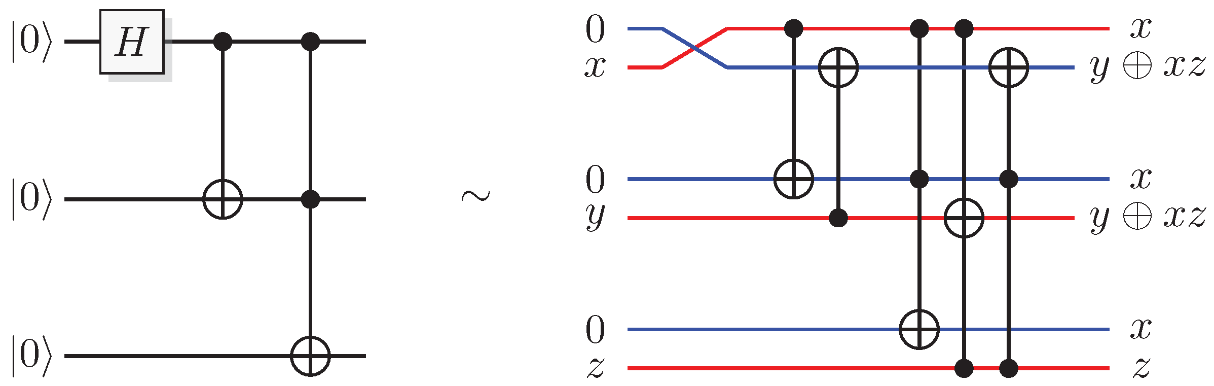
One construction that produces a GHZ-state, and the matching QSL construction.
Figure 17.
One construction that produces a GHZ-state, and the matching QSL construction.
Figure 18.
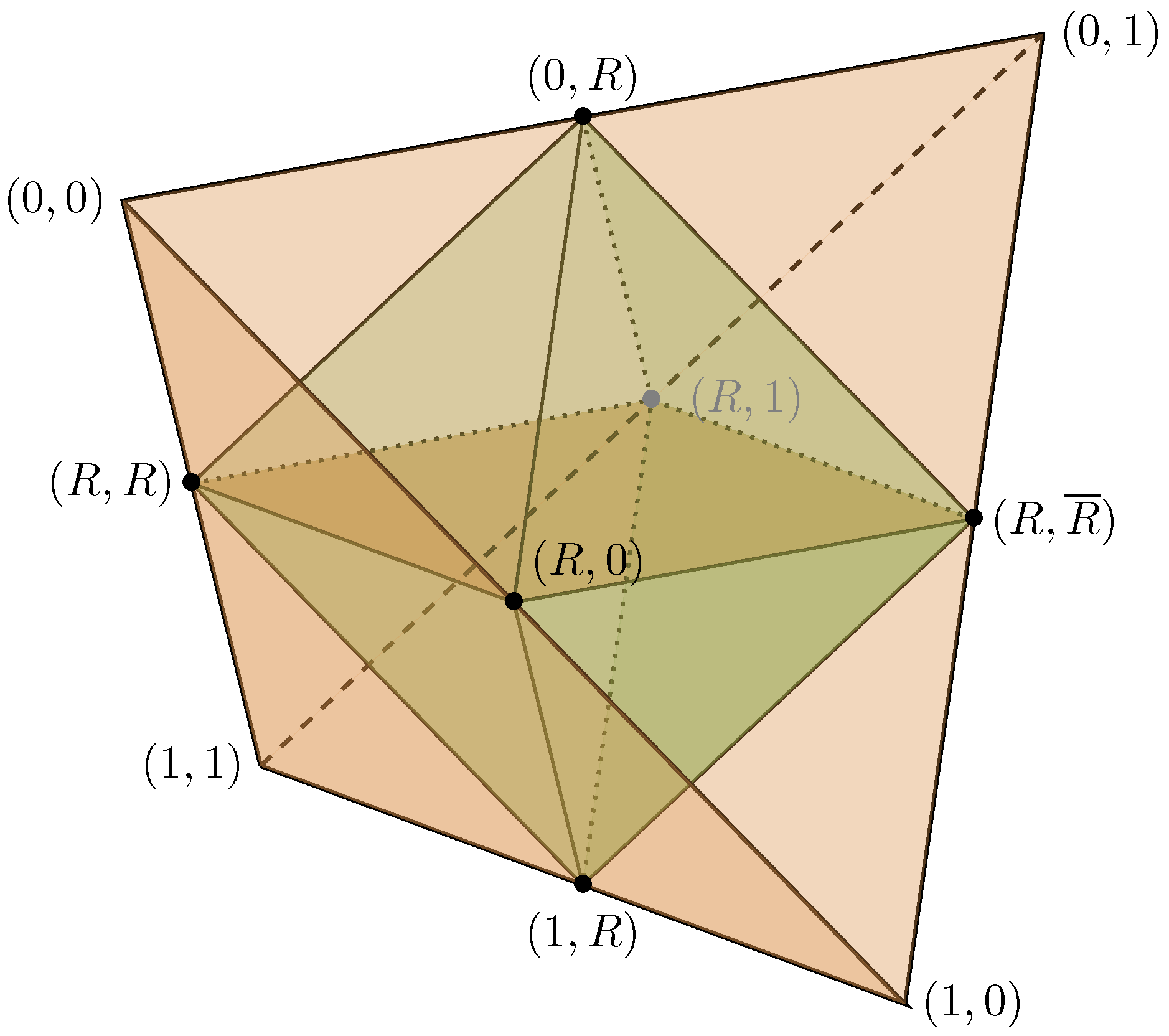
Representation of the state space of a single elementary system, with a geometry of a tetrahedron inscribing an octahedron. To aid with the visualization: if we take the vertices of the tetrahedron and fold them to one of the closest vertices on the octahedron, we recover the octahedron.
Figure 18.
Representation of the state space of a single elementary system, with a geometry of a tetrahedron inscribing an octahedron. To aid with the visualization: if we take the vertices of the tetrahedron and fold them to one of the closest vertices on the octahedron, we recover the octahedron.
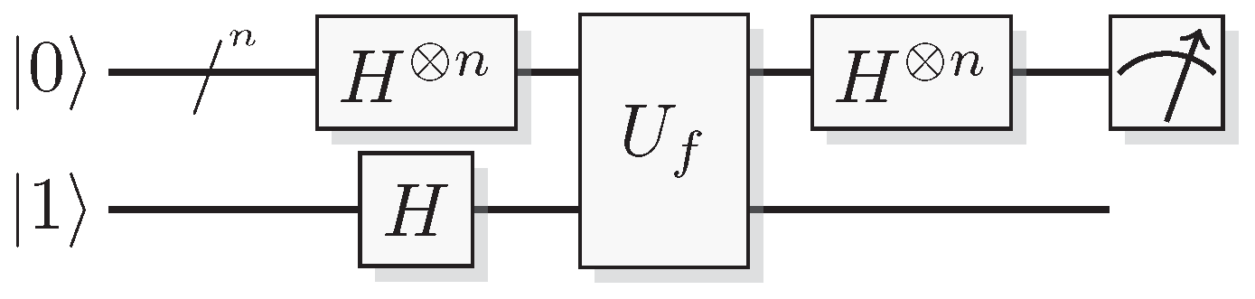
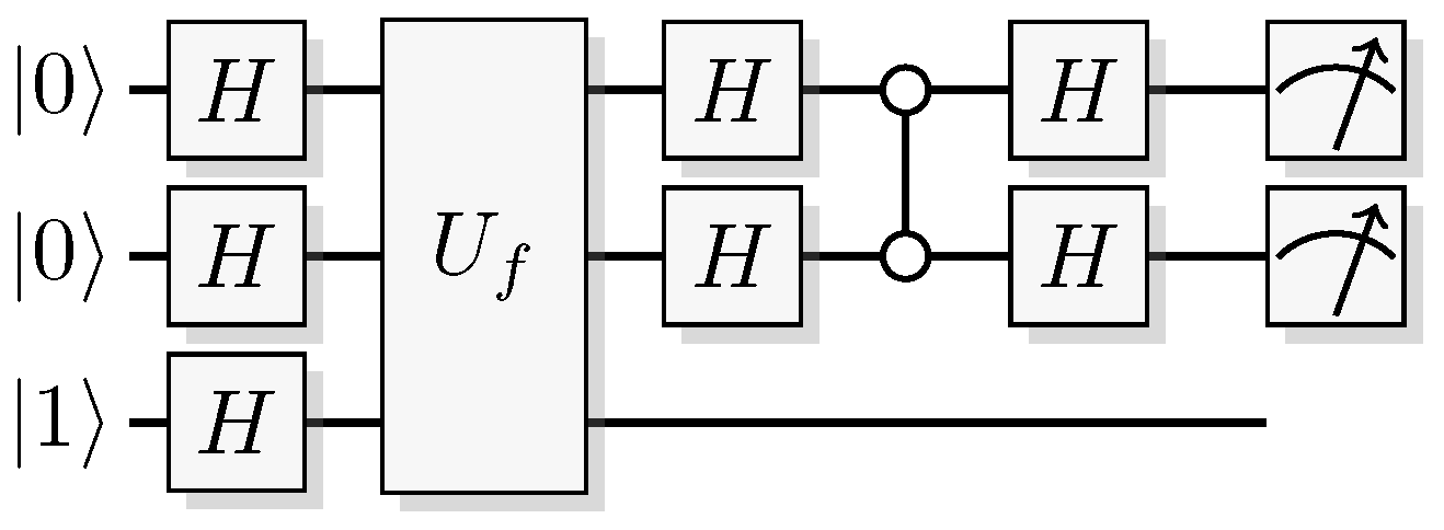
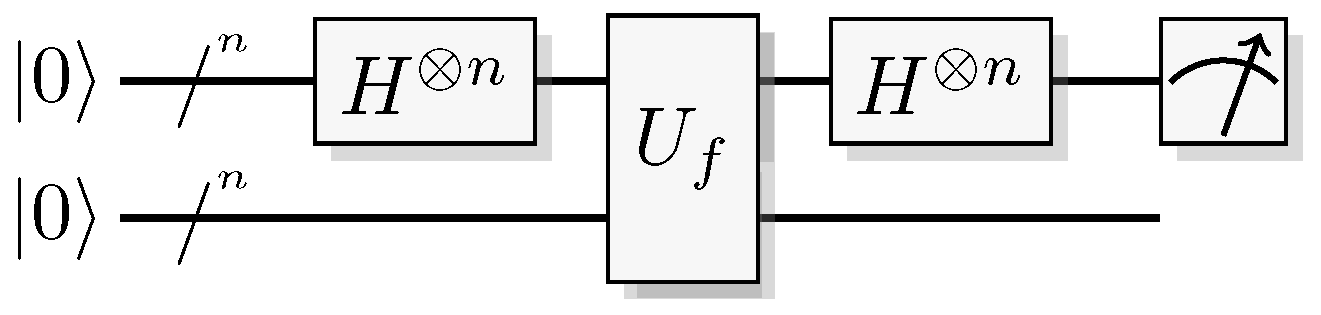
Figure 19.
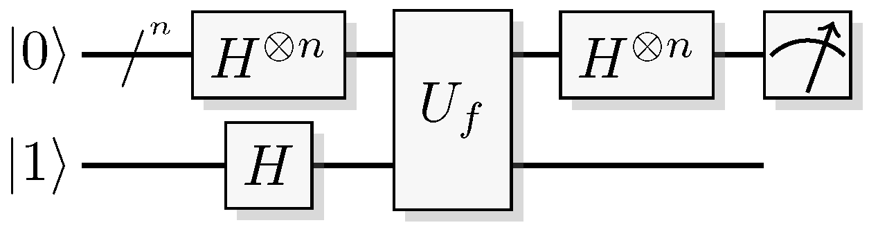
Quantum circuit for the Bernstein-Vazirani algorithm.
Figure 19.
Quantum circuit for the Bernstein-Vazirani algorithm.
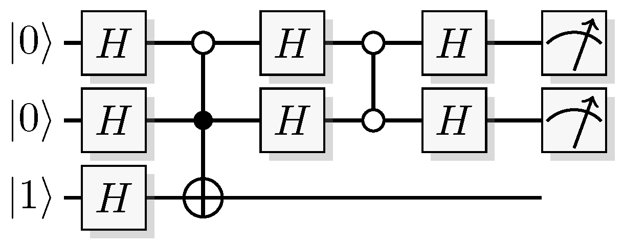
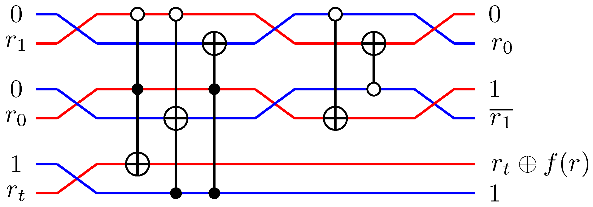
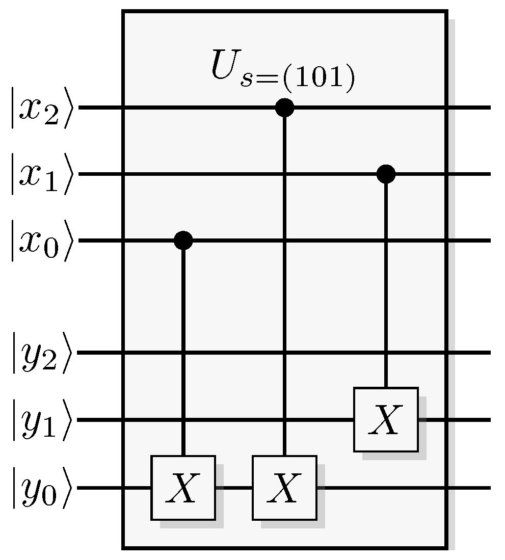
Figure 20.
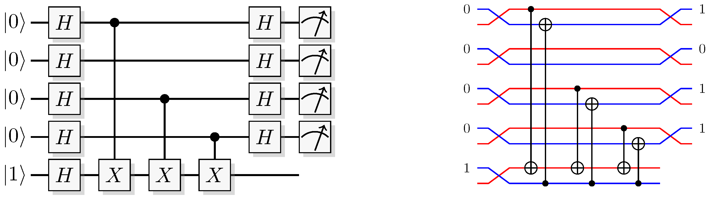
Example of a quantum and the corresponding QSL algorithm for solving the Bernstein-Vazirani problem when the secret string is . The unsigned red inputs and outputs of the QSL circuit are all uniformly distributed random bits.
Figure 20.
Example of a quantum and the corresponding QSL algorithm for solving the Bernstein-Vazirani problem when the secret string is . The unsigned red inputs and outputs of the QSL circuit are all uniformly distributed random bits.
Figure 21.
Circuit representation of the Deutsch-Jozsa algorithm.
Figure 21.
Circuit representation of the Deutsch-Jozsa algorithm.
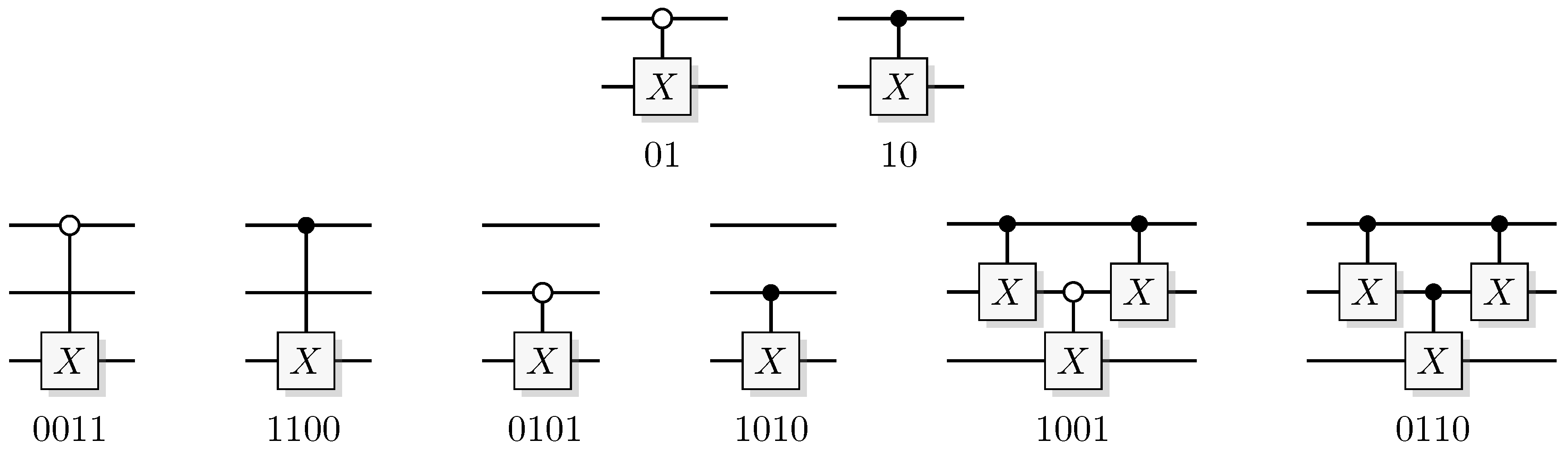
Figure 22.
Explicit implementations of all balanced oracles for the Deutsch-Jozsa algorithm for one and two-qubit input. White controls are inverted.
Figure 22.
Explicit implementations of all balanced oracles for the Deutsch-Jozsa algorithm for one and two-qubit input. White controls are inverted.
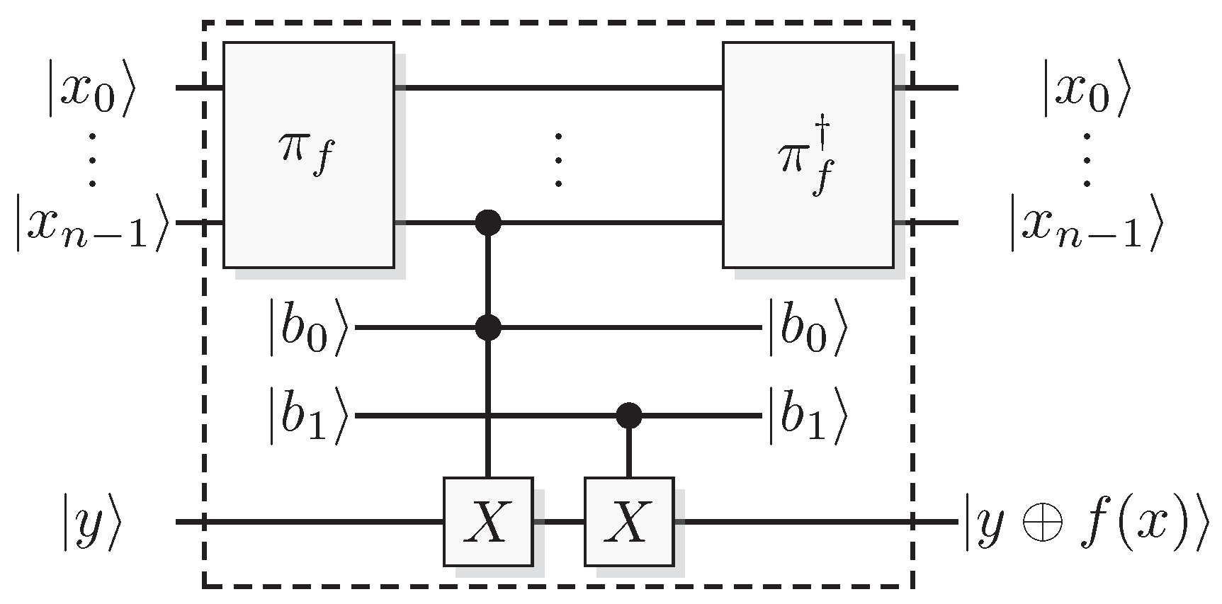
Figure 23.
A specific implementation of a quantum oracle that can be used to solve the Deutsch-Jozsa problem in Definition 2. The internal parameter chooses between a constant or balanced function, and if the function is constant, the value is . For balanced functions, the idea is that the first Toffoli acting as a CNOT to produce one specific balanced function (if the permutation is the identity), adding the most significant bit to the output, . Access to all balanced functions is then obtained by an arbitrary permutation of the output.
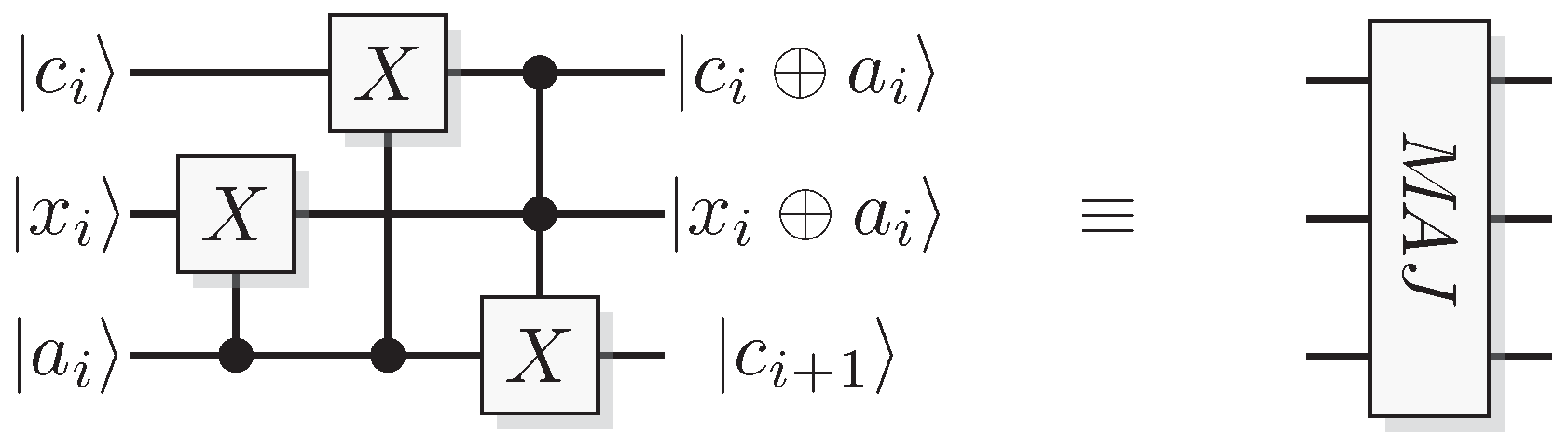
Figure 24.
A majority-function module where the output carry contains the majority value of the three input bits.
Figure 24.
A majority-function module where the output carry contains the majority value of the three input bits.
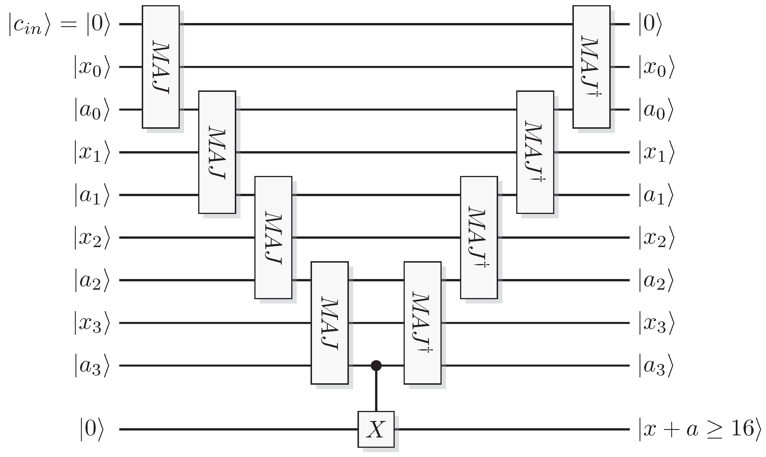
Figure 25.
Quantum circuit of a reversible comparator for comparing the sum of two 4-bit integers x and a to the number , signaling if in the answer register.
Figure 25.
Quantum circuit of a reversible comparator for comparing the sum of two 4-bit integers x and a to the number , signaling if in the answer register.
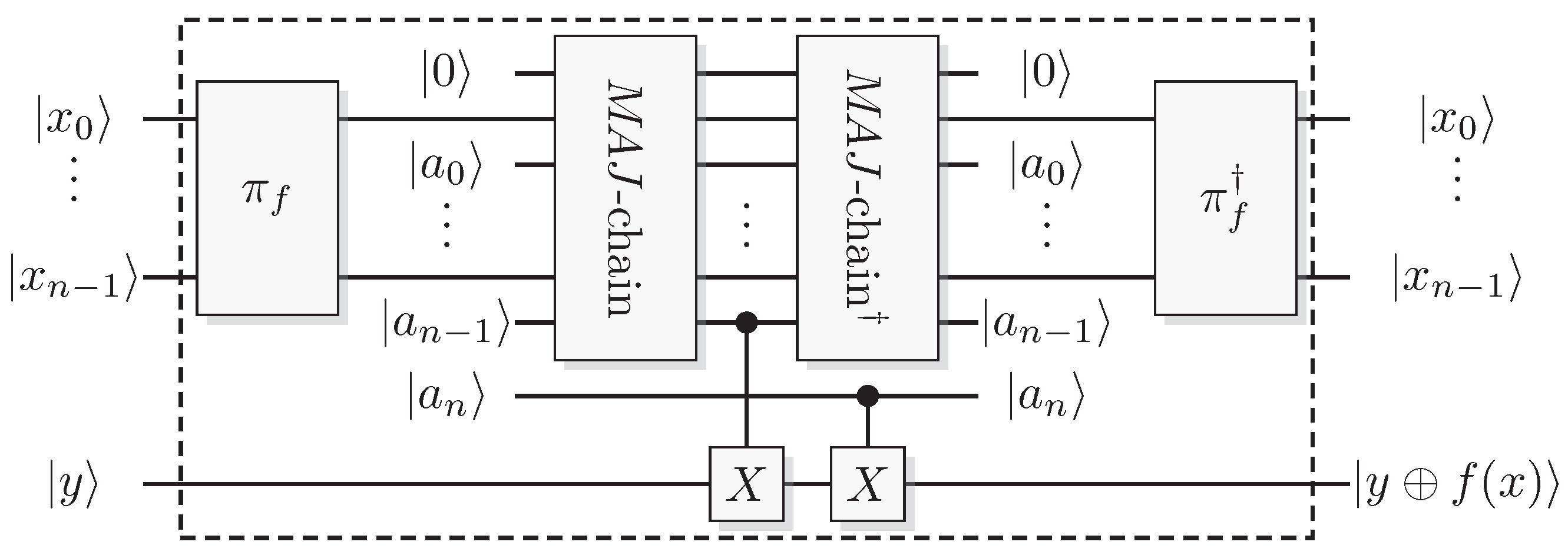
Figure 26.
Construction of a circuit that can give any Boolean function. The idea is to construct one specific Boolean function for each number
that gives the output 1 on
a inputs by using a comparator. Then produce the other functions by using a permutation of the input states. The comparator is built through two chains of
and
gates as in
Figure 25.
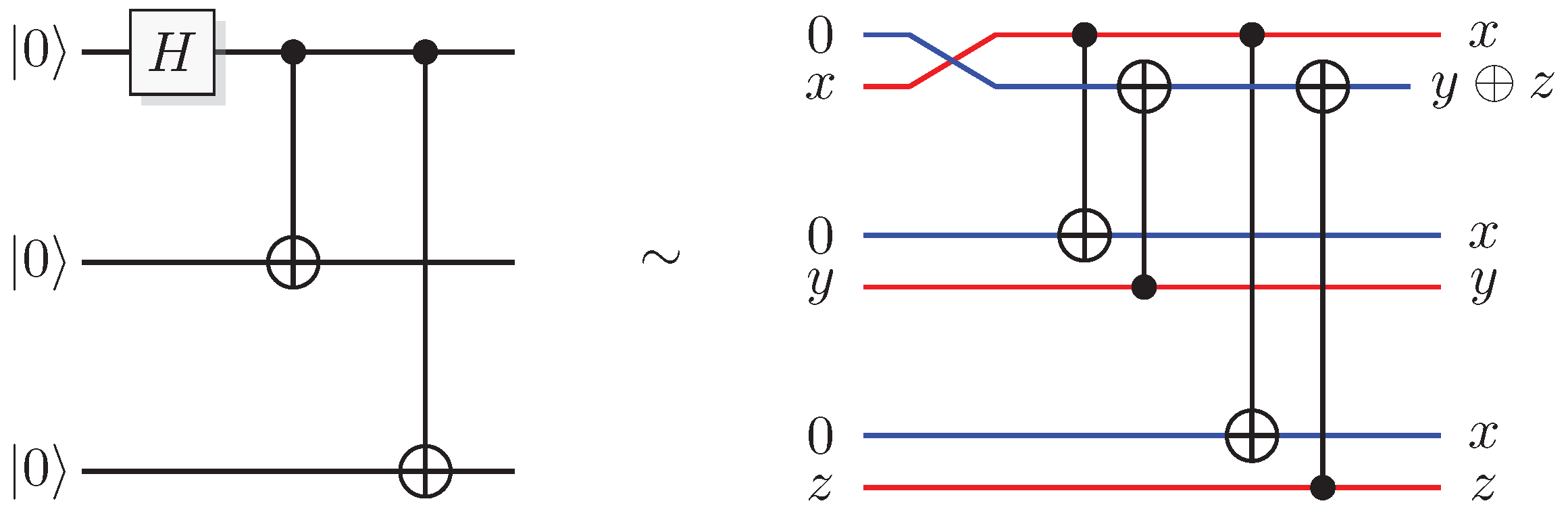
Figure 27.
Another construction that produces a GHZ-state, and the analogue construction in QSL.
Figure 27.
Another construction that produces a GHZ-state, and the analogue construction in QSL.
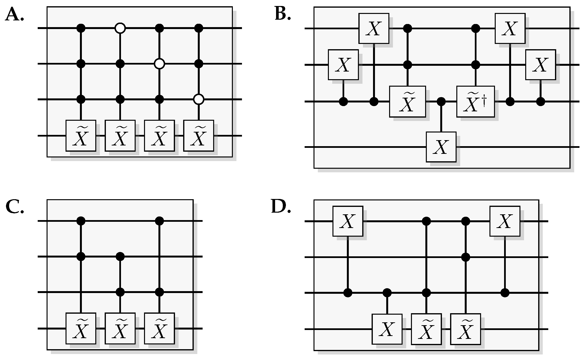
Figure 28.
Four different quantum circuit implementations of the same balanced function, computing the majority
(see
Figure 24) of three bits. (
A) Straightforward construction using four
gates. (
B) The majority is computed in place in the query register, the answer is copied out to the answer register, and the intermediate step is then uncomputed by applying
to the query register. (
C) is an optimization of A, tuned for as few gates as possible, and (
D) is another optimized for few Toffolis followed by few
s, generated as part of the list of all 72 possible functions in
Appendix A.
Figure 29.
Scheme for constructing a from three gates with a systematic error and an ancillary qubit initiated in .
Figure 29.
Scheme for constructing a from three gates with a systematic error and an ancillary qubit initiated in .
Figure 30.
Circuit for the one-shot Grover instance. The second-to-last gate is a two-qubit controlled phase flip (controlled-Z) with both controls inverted.
Figure 30.
Circuit for the one-shot Grover instance. The second-to-last gate is a two-qubit controlled phase flip (controlled-Z) with both controls inverted.
Figure 31.
Example circuit of the one-shot Grover where .
Figure 31.
Example circuit of the one-shot Grover where .
Figure 32.
QSL simulation of the one-shot Grover instance from
Figure 31.
Figure 32.
QSL simulation of the one-shot Grover instance from
Figure 31.
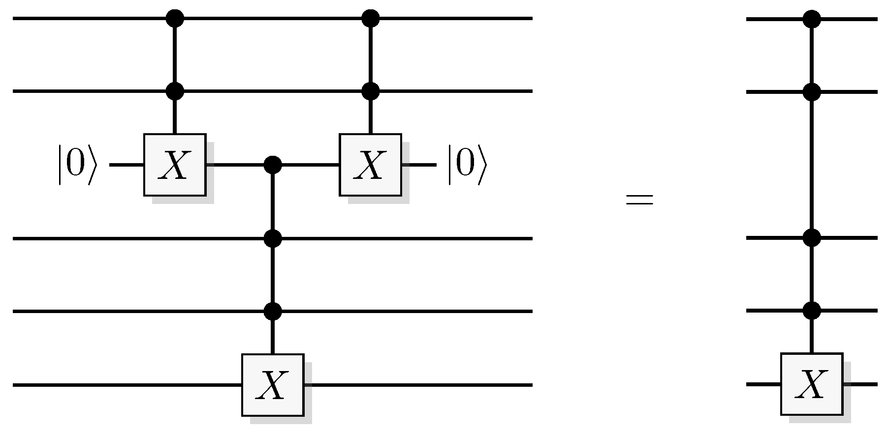
Figure 33.
Scheme for construction a 3-Toffoli from three regular Toffoli gates and an ancillary qubit initiated in .
Figure 33.
Scheme for construction a 3-Toffoli from three regular Toffoli gates and an ancillary qubit initiated in .
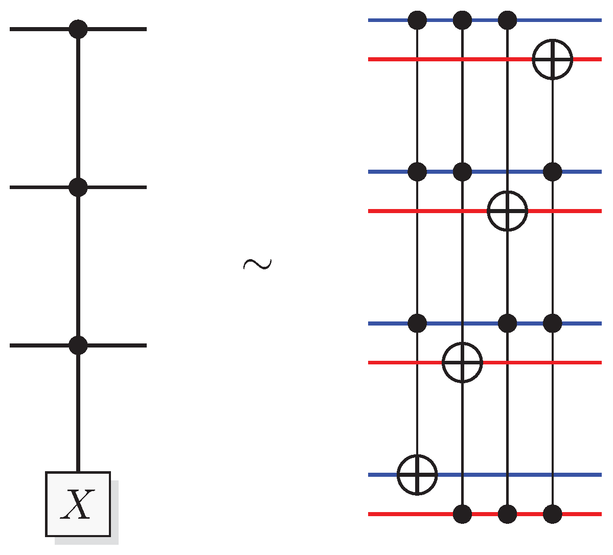
Figure 34.
QSL identity for the 3-Toffoli.
Figure 34.
QSL identity for the 3-Toffoli.
Figure 35.
Scheme for construction a 4-Toffoli from one 3-Toffoli, two regular Toffoli gates, and an ancillary qubit initiated in .
Figure 35.
Scheme for construction a 4-Toffoli from one 3-Toffoli, two regular Toffoli gates, and an ancillary qubit initiated in .
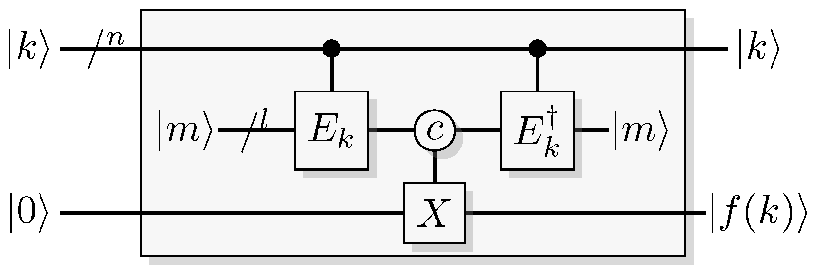
Figure 36.
Circuit construction for using Grover’s algorithm to perform a known plaintext attack on a symmetric cipher , where the key k has a bitsize of n and the known plaintext a bitsize of l. The control labeled c expresses that X is applied only if the output of is , inverting the target bit. This can be constructed with an l-Toffoli with regular and inverted controls.
Figure 37.
Quantum circuit used as a subroutine in Simon’s algorithm. The subroutine assumes oracle access to .
Figure 37.
Quantum circuit used as a subroutine in Simon’s algorithm. The subroutine assumes oracle access to .
Figure 38.
Example construction for , where and .
Figure 38.
Example construction for , where and .
Figure 39.
Oracle construction for Simon’s Subroutine.
Figure 39.
Oracle construction for Simon’s Subroutine.
Figure 40.
Oracle construction for Simons algorithm where the output can be initiated in a non-zero state. The boxed modulo 2 addition denotes an array of CNOTs that adds each ancilla bit to the corresponding target bit.
Figure 40.
Oracle construction for Simons algorithm where the output can be initiated in a non-zero state. The boxed modulo 2 addition denotes an array of CNOTs that adds each ancilla bit to the corresponding target bit.
Figure 41.
Proposed quantum circuit as subroutine in an algorithm solving Simon’s problem in polynomial time, both in quantum theory, and in QSL.
Figure 41.
Proposed quantum circuit as subroutine in an algorithm solving Simon’s problem in polynomial time, both in quantum theory, and in QSL.
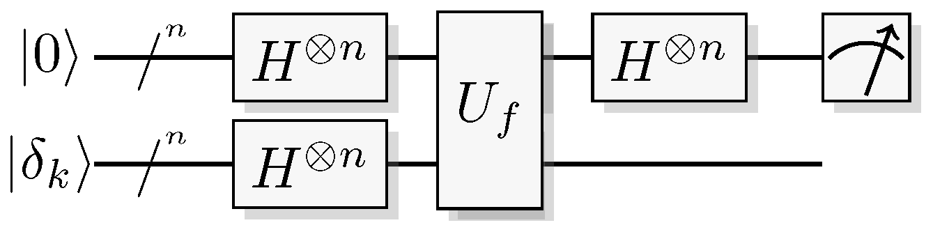
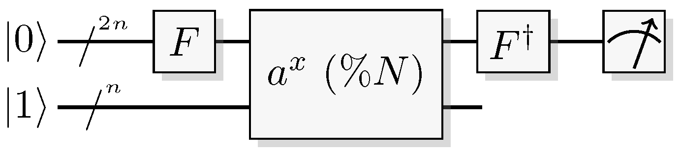
Figure 42.
Circuit diagram of the quantum subroutine used in Shor’s algorithm. A -qubit register is initiated in the zero-state , and an n-qubit register in . Basis change of the input-register part of the controlled modular exponentiation operator allow for sampling a probability distribution with peaks at .
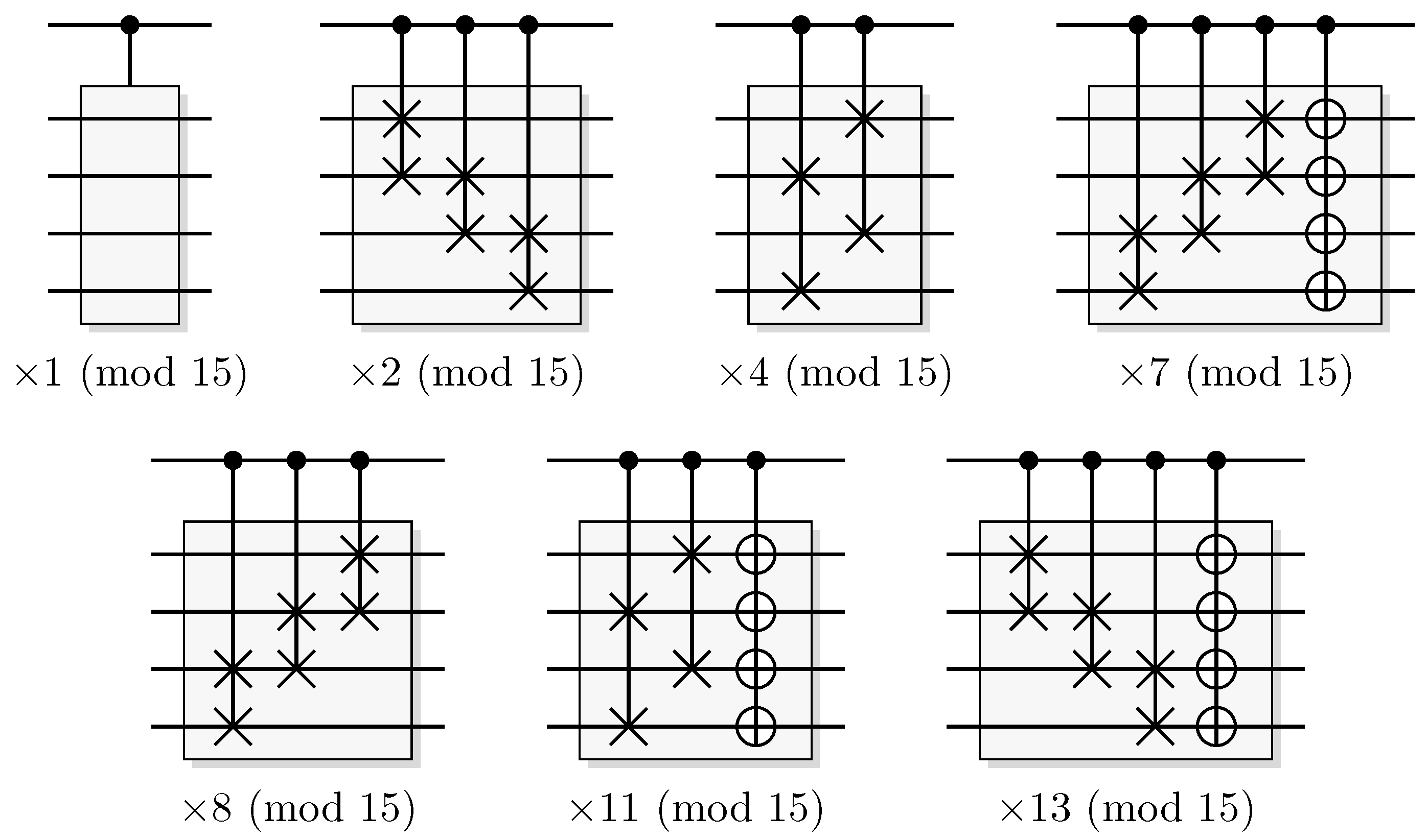
Figure 43.
Controlled modular multipliers that occur in Shor’s algorithm.
Figure 43.
Controlled modular multipliers that occur in Shor’s algorithm.
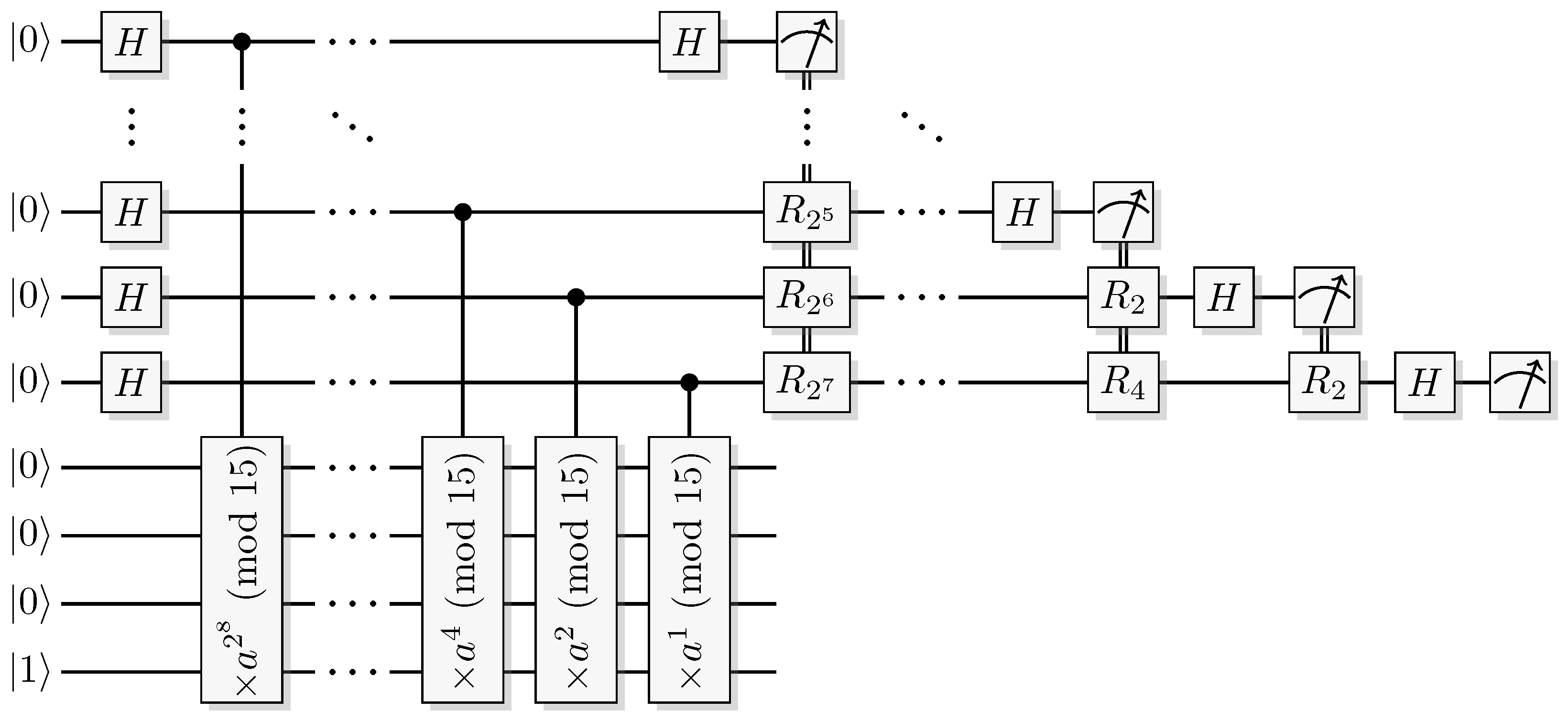
Figure 44.
Shor’s algorithm with semiclassical inverse Fourier transform. Please note that and (mod 15), so that many of the controlled multiplications will be identities. Therefore, most rotations will never be applied (in the ideal situation), in fact only the very last operation can ever occur.
Figure 44.
Shor’s algorithm with semiclassical inverse Fourier transform. Please note that and (mod 15), so that many of the controlled multiplications will be identities. Therefore, most rotations will never be applied (in the ideal situation), in fact only the very last operation can ever occur.
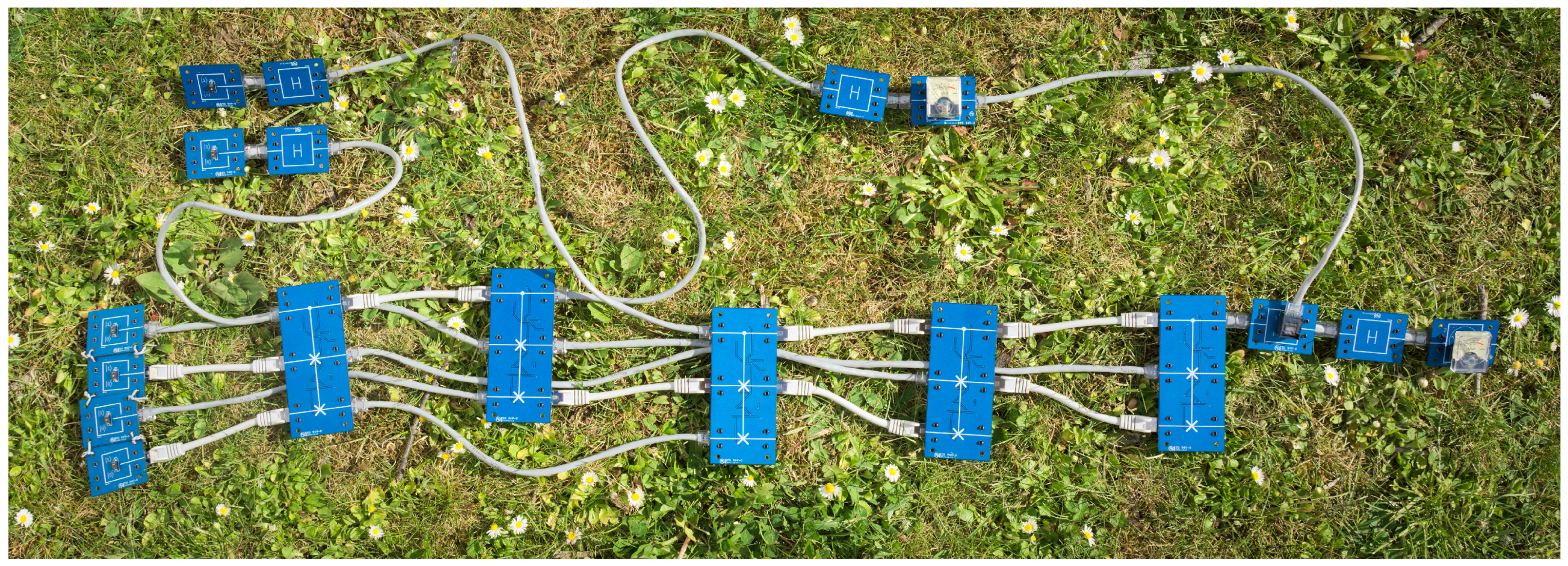
Figure 45.
Hardware realization QSL simulation of Shor’s algorithm. For the case so that the modular multipliers used are, (mod 15), and (mod 15).
Figure 45.
Hardware realization QSL simulation of Shor’s algorithm. For the case so that the modular multipliers used are, (mod 15), and (mod 15).
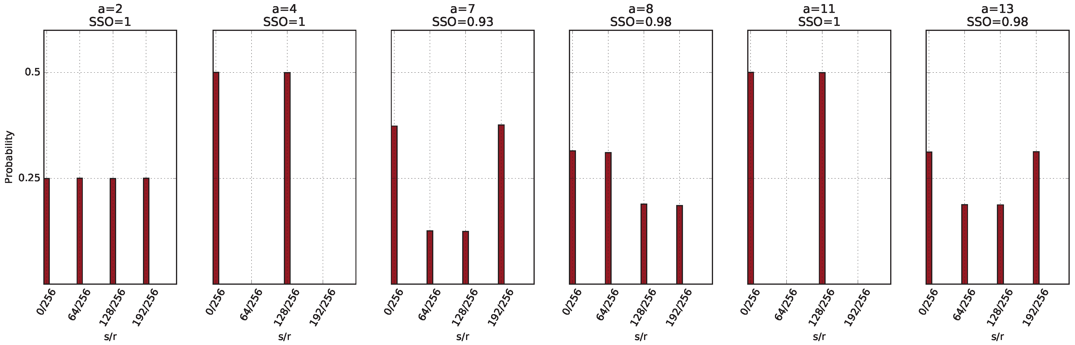
Figure 46.
Estimated output probability. Point estimates of the output probability distributions of the subroutine, for the non-trivial elements in the multiplicative group of integers mod 15. Each distribution is estimated from samples.
Figure 46.
Estimated output probability. Point estimates of the output probability distributions of the subroutine, for the non-trivial elements in the multiplicative group of integers mod 15. Each distribution is estimated from samples.


