Universal Target Learning: An Efficient and Effective Technique for Semi-Naive Bayesian Learning


Abstract
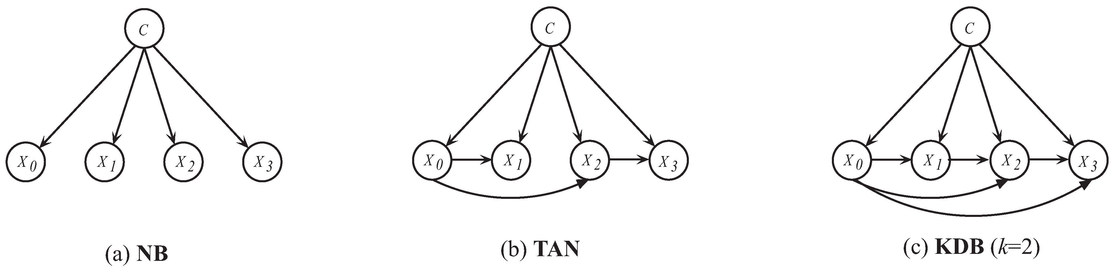
1. Introduction
2. Preliminaries
3. UKDB: Universal Target Learning
3.1. Target Learning (TL)
| Algorithm 1: The learning procedure of KDB. |
 |
| Algorithm 2: The learning procedure of KDB. |
 |
3.2. Universal Target Learning
| Algorithm 3: UKDB. |
 |
| Algorithm 4: UKDB. |
 |
4. Results and Discussion
- NB, the standard Naive Bayes.
- TAN, Tree-Augmented Naive Bayes.
- , k-dependence Bayesian classifier with k = 1.
- , k-dependence Bayesian classifier with k = 2.
- AODE, Averaged One-Dependence Estimators.
- WATAN, the Weighted Averaged Tree-Augmented Naive Bayes.
- TANe, an ensemble Tree-Augmented Naive Bayes applying target learning.
- , k-dependence Bayesian classifier with k = 1 in the framework of UTL.
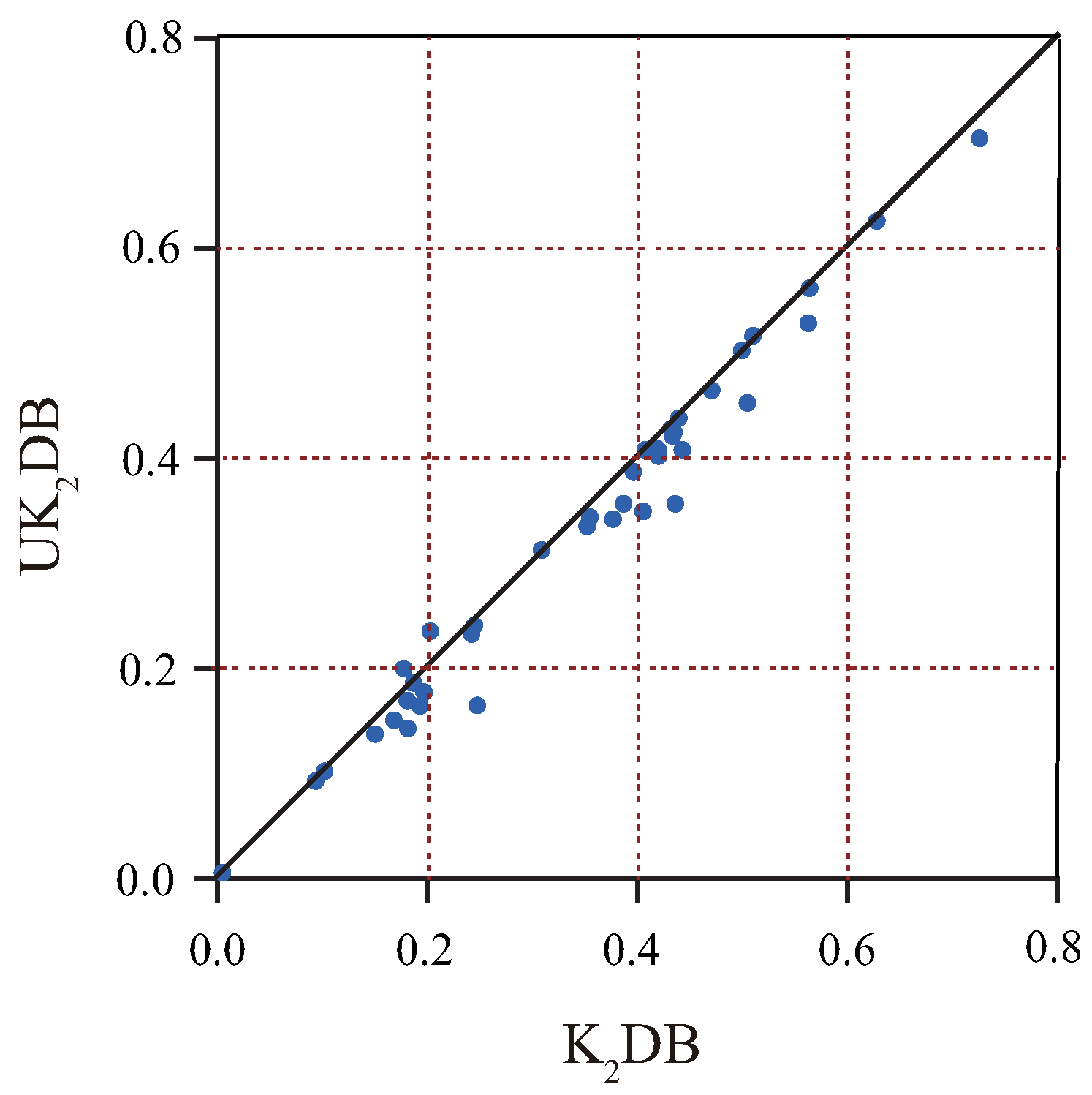
- , k-dependence Bayesian classifier with k = 2 in the framework of UTL.
4.1. Comparison of Zero-One Loss, RMSE, and -Score
4.1.1. Zero-One Loss
4.1.2. RMSE
4.1.3. -Score
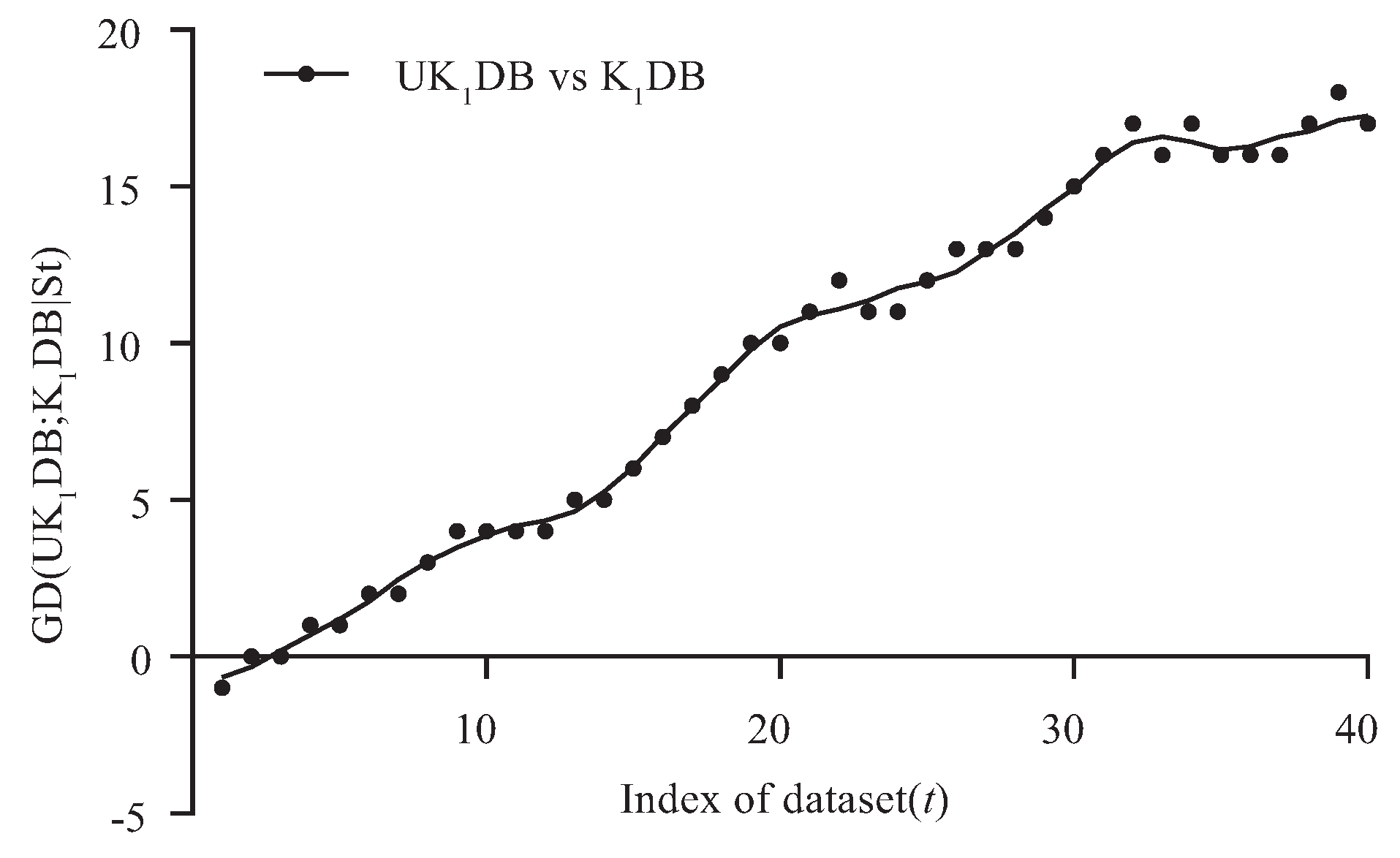
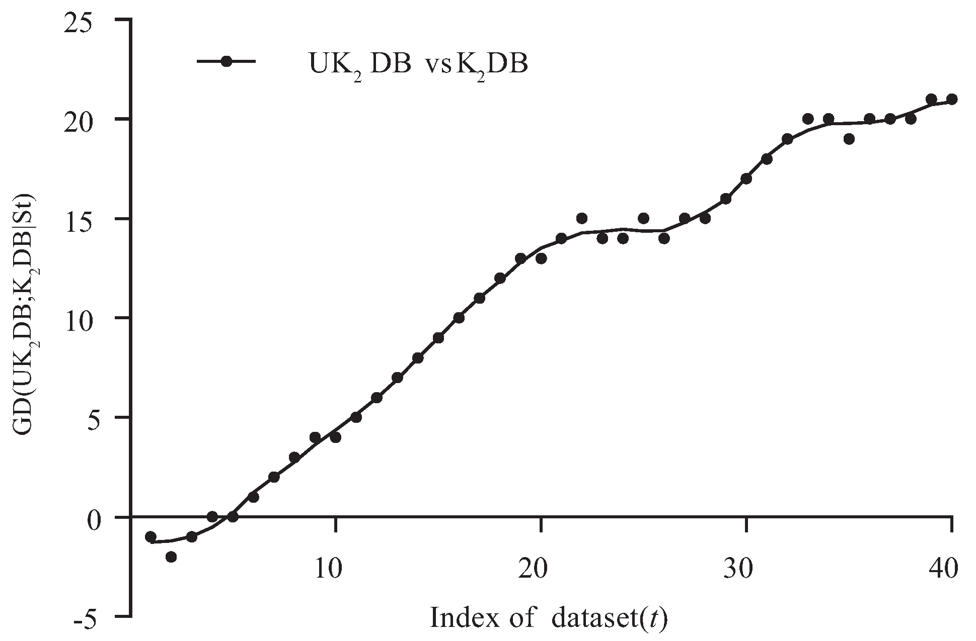
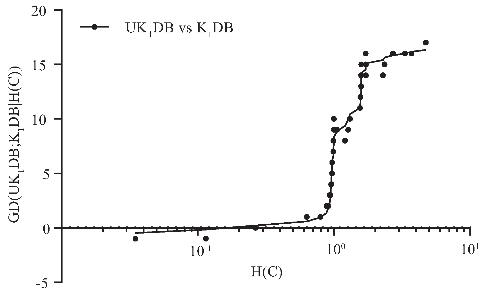
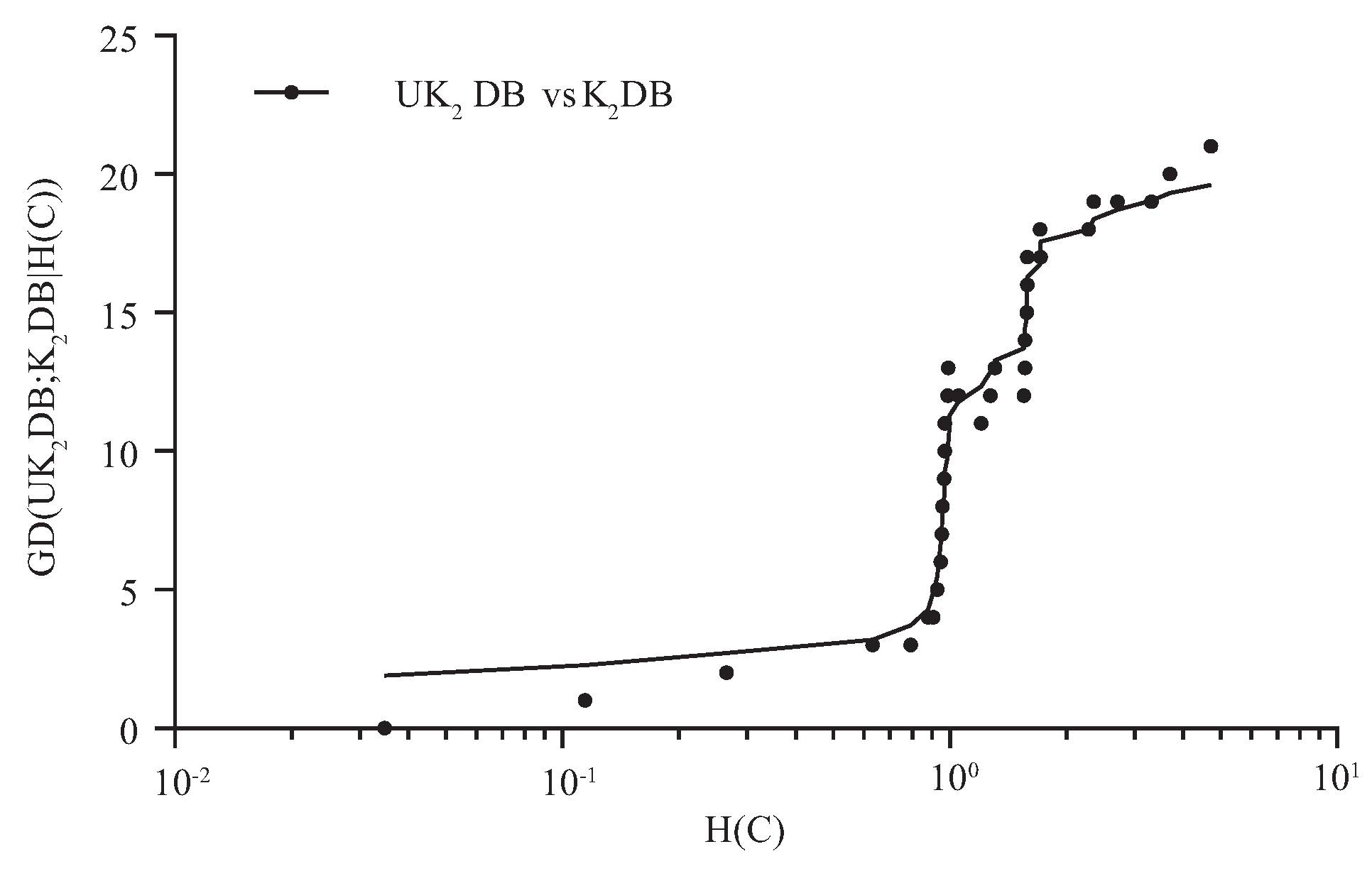
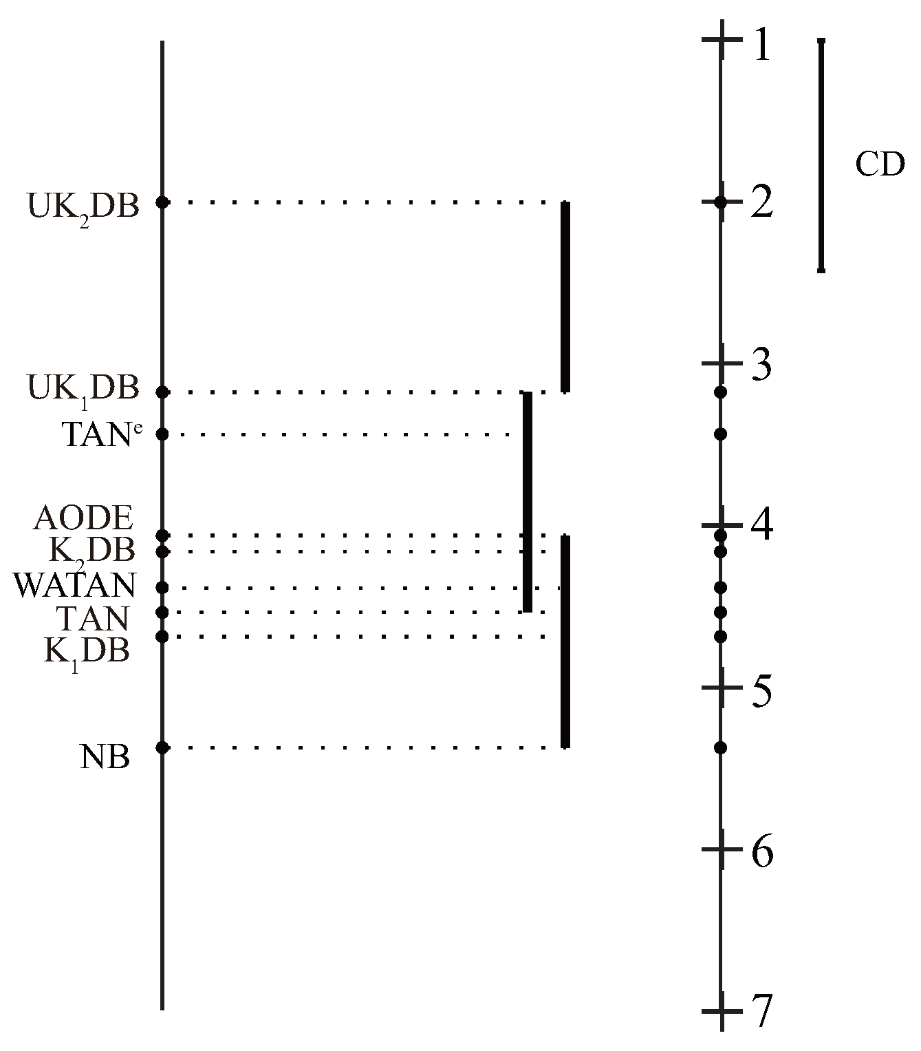
4.2. Goal Difference
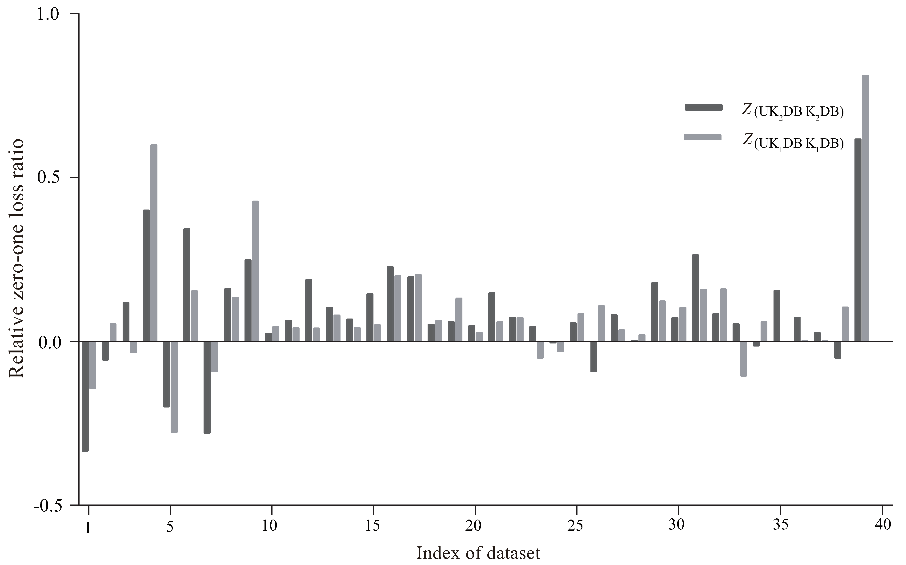
4.3. Relative Zero-One Loss Ratio
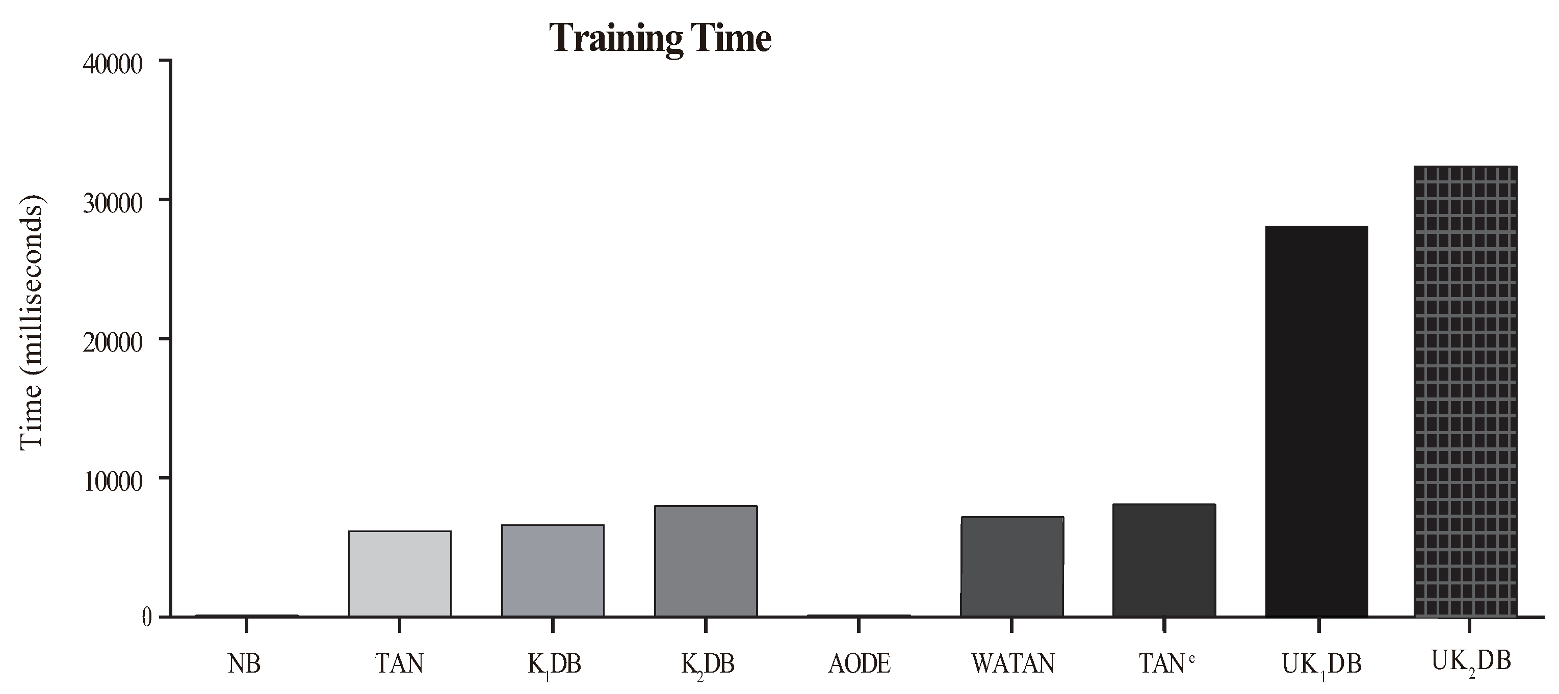
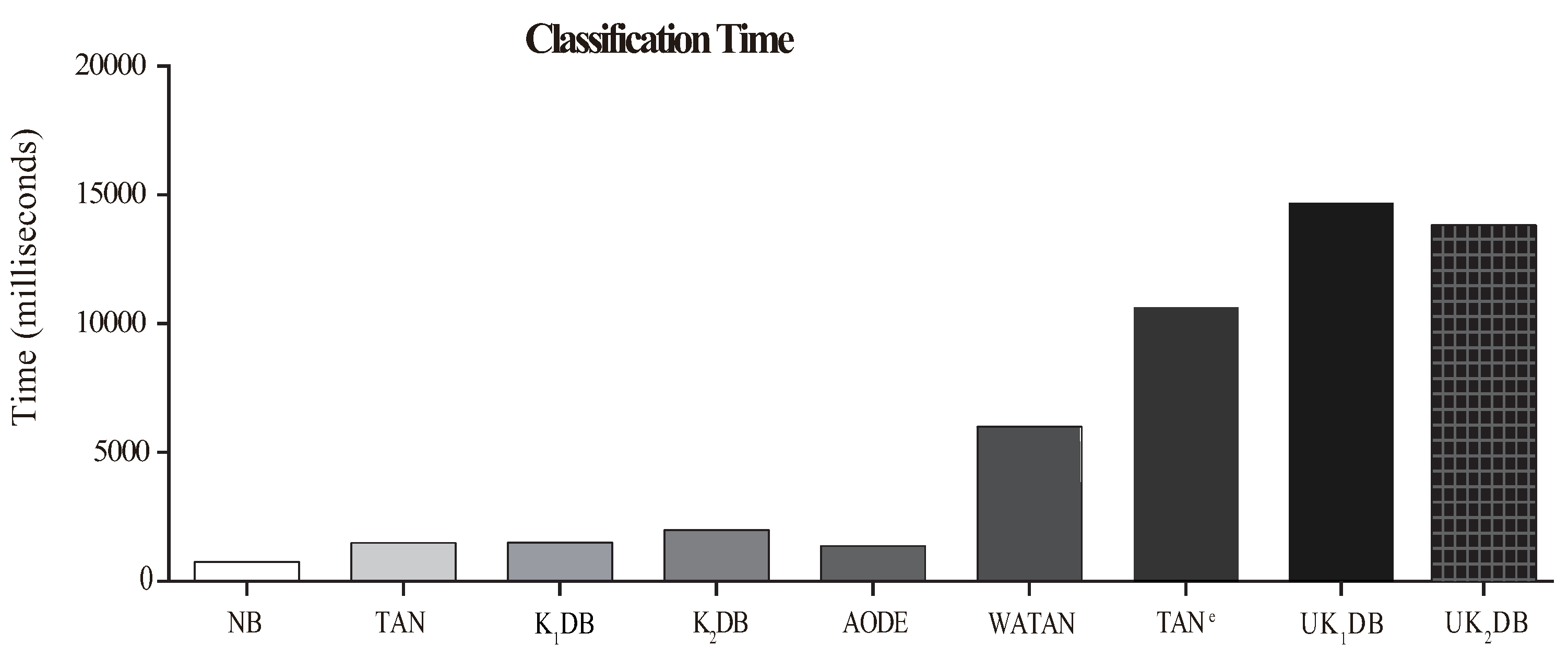
4.4. Training and Classification Time
4.5. Global Comparison
5. Conclusions and Future Work
Author Contributions
Funding
Conflicts of Interest
Appendix A

| Index | Datasets | NB | TAN | AODE | WATAN | TANe | KDB | KDB | UKDB | UKDB |
|---|---|---|---|---|---|---|---|---|---|---|
| 1 | contact-lenses | 0.3750 | 0.3750 | 0.3750 | 0.4583 | 0.3750 | 0.2917 | 0.2500 | 0.3333 | 0.3333 |
| 2 | lung-cancer | 0.4375 | 0.5938 | 0.5000 | 0.6250 | 0.6563 | 0.5938 | 0.5625 | 0.5625 | 0.5938 |
| 3 | post-operative | 0.3444 | 0.3667 | 0.3333 | 0.3667 | 0.3444 | 0.3444 | 0.3778 | 0.3556 | 0.3333 |
| 4 | zoo | 0.0297 | 0.0099 | 0.0297 | 0.0198 | 0.0099 | 0.0495 | 0.0495 | 0.0198 | 0.0297 |
| 5 | echocardiogram | 0.3359 | 0.3282 | 0.3206 | 0.3282 | 0.3282 | 0.3053 | 0.3435 | 0.3206 | 0.3282 |
| 6 | lymphography | 0.1486 | 0.1757 | 0.1689 | 0.1689 | 0.1689 | 0.1757 | 0.2365 | 0.1486 | 0.1554 |
| 7 | iris | 0.0867 | 0.0800 | 0.0867 | 0.0800 | 0.0867 | 0.0867 | 0.0867 | 0.0867 | 0.0733 |
| 8 | teaching-ae | 0.4967 | 0.5497 | 0.4901 | 0.5364 | 0.5166 | 0.5430 | 0.5364 | 0.4702 | 0.4503 |
| 9 | wine | 0.0169 | 0.0337 | 0.0225 | 0.0337 | 0.0337 | 0.0393 | 0.0225 | 0.0225 | 0.0169 |
| 10 | autos | 0.3122 | 0.2146 | 0.2049 | 0.2146 | 0.2000 | 0.2146 | 0.2049 | 0.2049 | 0.2000 |
| 11 | glass-id | 0.2617 | 0.2196 | 0.2523 | 0.2196 | 0.2103 | 0.2243 | 0.2196 | 0.2150 | 0.2056 |
| 12 | hungarian | 0.1599 | 0.1701 | 0.1667 | 0.1735 | 0.1599 | 0.1701 | 0.1803 | 0.1633 | 0.1463 |
| 13 | heart-disease-c | 0.1815 | 0.2079 | 0.2013 | 0.2046 | 0.1881 | 0.2079 | 0.2244 | 0.1914 | 0.2013 |
| 14 | primary-tumor | 0.5457 | 0.5428 | 0.5752 | 0.5428 | 0.5575 | 0.5693 | 0.5723 | 0.5457 | 0.5339 |
| 15 | horse-colic | 0.2174 | 0.2092 | 0.2011 | 0.2120 | 0.2038 | 0.2174 | 0.2446 | 0.2065 | 0.2092 |
| 16 | house-votes-84 | 0.0943 | 0.0552 | 0.0529 | 0.0529 | 0.0552 | 0.0690 | 0.0506 | 0.0552 | 0.0391 |
| 17 | cylinder-bands | 0.2148 | 0.2833 | 0.1889 | 0.2463 | 0.1833 | 0.2278 | 0.2259 | 0.1815 | 0.1815 |
| 18 | balance-scale | 0.2720 | 0.2736 | 0.2832 | 0.2736 | 0.2784 | 0.2816 | 0.2784 | 0.2640 | 0.2640 |
| 19 | credit-a | 0.1406 | 0.1507 | 0.1391 | 0.1507 | 0.1391 | 0.1551 | 0.1464 | 0.1348 | 0.1377 |
| 20 | pima-ind-diabetes | 0.2448 | 0.2383 | 0.2383 | 0.2370 | 0.2383 | 0.2422 | 0.2448 | 0.2357 | 0.2331 |
| 21 | tic-tac-toe | 0.3069 | 0.2286 | 0.2651 | 0.2265 | 0.2724 | 0.2463 | 0.2035 | 0.2317 | 0.1733 |
| 22 | german | 0.2530 | 0.2730 | 0.2480 | 0.2760 | 0.2590 | 0.2760 | 0.2890 | 0.2560 | 0.2680 |
| 23 | car | 0.1400 | 0.0567 | 0.0816 | 0.0567 | 0.0579 | 0.0567 | 0.0382 | 0.0741 | 0.0723 |
| 24 | mfeat-mor | 0.3140 | 0.2970 | 0.3145 | 0.2980 | 0.3050 | 0.2990 | 0.3060 | 0.3080 | 0.3070 |
| 25 | hypothyroid | 0.0149 | 0.0104 | 0.0136 | 0.0104 | 0.0092 | 0.0107 | 0.0107 | 0.0098 | 0.0101 |
| 26 | kr-vs-kp | 0.1214 | 0.0776 | 0.0842 | 0.0776 | 0.0566 | 0.0544 | 0.0416 | 0.0485 | 0.0454 |
| 27 | dis | 0.0159 | 0.0159 | 0.0130 | 0.0154 | 0.0162 | 0.0146 | 0.0138 | 0.0141 | 0.0127 |
| 28 | abalone | 0.4762 | 0.4587 | 0.4472 | 0.4582 | 0.4554 | 0.4633 | 0.4563 | 0.4539 | 0.4554 |
| 29 | waveform-5000 | 0.2006 | 0.1844 | 0.1462 | 0.1844 | 0.1650 | 0.1820 | 0.2000 | 0.1598 | 0.1642 |
| 30 | phoneme | 0.2615 | 0.2733 | 0.2392 | 0.2345 | 0.2429 | 0.2120 | 0.1984 | 0.1901 | 0.1841 |
| 31 | wall-following | 0.1054 | 0.0554 | 0.0370 | 0.0550 | 0.0462 | 0.0462 | 0.0401 | 0.0389 | 0.0295 |
| 32 | page-blocks | 0.0619 | 0.0415 | 0.0338 | 0.0418 | 0.0342 | 0.0433 | 0.0391 | 0.0364 | 0.0358 |
| 33 | thyroid | 0.1111 | 0.0720 | 0.0701 | 0.0723 | 0.0726 | 0.0693 | 0.0706 | 0.0835 | 0.0669 |
| 34 | sign | 0.3586 | 0.2755 | 0.2821 | 0.2752 | 0.2713 | 0.2881 | 0.2539 | 0.2713 | 0.2572 |
| 35 | nursery | 0.0973 | 0.0654 | 0.0730 | 0.0654 | 0.0617 | 0.0654 | 0.0289 | 0.0702 | 0.0555 |
| 36 | seer_mdl | 0.2379 | 0.2376 | 0.2328 | 0.2374 | 0.2332 | 0.2367 | 0.2555 | 0.2363 | 0.2367 |
| 37 | adult | 0.1592 | 0.1380 | 0.1493 | 0.1380 | 0.1326 | 0.1385 | 0.1383 | 0.1382 | 0.1347 |
| 38 | localization | 0.4955 | 0.3575 | 0.3596 | 0.3575 | 0.3610 | 0.3706 | 0.2964 | 0.3319 | 0.3112 |
| 39 | poker-hand | 0.4988 | 0.3295 | 0.4812 | 0.3295 | 0.0763 | 0.3291 | 0.1961 | 0.0618 | 0.0752 |
| 40 | donation | 0.0002 | 0.0000 | 0.0002 | 0.0000 | 0.0000 | 0.0000 | 0.0000 | 0.0001 | 0.0000 |
| Index | Datasets | NB | TAN | AODE | WATAN | TANe | KDB | KDB | UKDB | UKDB |
|---|---|---|---|---|---|---|---|---|---|---|
| 1 | contact-lenses | 0.5017 | 0.6077 | 0.5258 | 0.5737 | 0.5736 | 0.5024 | 0.4996 | 0.5136 | 0.5033 |
| 2 | lung-cancer | 0.6431 | 0.7623 | 0.6915 | 0.7662 | 0.7069 | 0.7523 | 0.7313 | 0.6942 | 0.7391 |
| 3 | post-operative | 0.5103 | 0.5340 | 0.5215 | 0.5358 | 0.5157 | 0.5289 | 0.5632 | 0.5256 | 0.5289 |
| 4 | zoo | 0.1623 | 0.1309 | 0.1536 | 0.1341 | 0.1313 | 0.1984 | 0.1815 | 0.1426 | 0.1428 |
| 5 | echocardiogram | 0.4896 | 0.4886 | 0.4903 | 0.4890 | 0.4852 | 0.4846 | 0.4889 | 0.4878 | 0.4891 |
| 6 | lymphography | 0.3465 | 0.3813 | 0.3556 | 0.3857 | 0.3761 | 0.3726 | 0.4362 | 0.3614 | 0.3571 |
| 7 | iris | 0.2545 | 0.2441 | 0.2544 | 0.2435 | 0.2505 | 0.2435 | 0.2447 | 0.2628 | 0.2407 |
| 8 | teaching-ae | 0.6204 | 0.6300 | 0.6117 | 0.6242 | 0.6191 | 0.6332 | 0.6286 | 0.6286 | 0.6262 |
| 9 | wine | 0.1134 | 0.1746 | 0.1245 | 0.1748 | 0.1583 | 0.1761 | 0.1501 | 0.1355 | 0.1374 |
| 10 | autos | 0.5190 | 0.4475 | 0.4397 | 0.4420 | 0.4362 | 0.4460 | 0.4399 | 0.4252 | 0.4385 |
| 11 | glass-id | 0.4353 | 0.4109 | 0.4235 | 0.4087 | 0.4036 | 0.4223 | 0.4205 | 0.4179 | 0.4020 |
| 12 | hungarian | 0.3667 | 0.3429 | 0.3476 | 0.3418 | 0.3315 | 0.3380 | 0.3552 | 0.3534 | 0.3444 |
| 13 | heart-disease-c | 0.3743 | 0.3775 | 0.3659 | 0.3783 | 0.3583 | 0.3810 | 0.3963 | 0.3802 | 0.3877 |
| 14 | primary-tumor | 0.7084 | 0.7170 | 0.7155 | 0.7166 | 0.7154 | 0.7190 | 0.7262 | 0.7085 | 0.7048 |
| 15 | horse-colic | 0.4209 | 0.4205 | 0.4015 | 0.4215 | 0.3951 | 0.4131 | 0.4348 | 0.4164 | 0.4247 |
| 16 | house-votes-84 | 0.2997 | 0.2181 | 0.1994 | 0.2181 | 0.2126 | 0.2235 | 0.1969 | 0.2221 | 0.1779 |
| 17 | cylinder-bands | 0.4291 | 0.4358 | 0.4080 | 0.4277 | 0.3973 | 0.4435 | 0.4431 | 0.4077 | 0.4083 |
| 18 | balance-scale | 0.4431 | 0.4344 | 0.4350 | 0.4344 | 0.4414 | 0.4384 | 0.4323 | 0.4279 | 0.4286 |
| 19 | credit-a | 0.3350 | 0.3415 | 0.3271 | 0.3407 | 0.3300 | 0.3416 | 0.3480 | 0.3336 | 0.3355 |
| 20 | pima-ind-diabetes | 0.4147 | 0.4059 | 0.4078 | 0.4059 | 0.4044 | 0.4054 | 0.4074 | 0.4095 | 0.4082 |
| 21 | tic-tac-toe | 0.4309 | 0.4023 | 0.3995 | 0.4023 | 0.4216 | 0.4050 | 0.3772 | 0.4134 | 0.3421 |
| 22 | german | 0.4204 | 0.4367 | 0.4161 | 0.4373 | 0.4206 | 0.4389 | 0.4665 | 0.4364 | 0.4531 |
| 23 | car | 0.3395 | 0.2405 | 0.3022 | 0.2406 | 0.2565 | 0.2404 | 0.2031 | 0.2426 | 0.2358 |
| 24 | mfeat-mor | 0.4817 | 0.4657 | 0.4710 | 0.4660 | 0.4686 | 0.4665 | 0.4707 | 0.4673 | 0.4652 |
| 25 | hypothyroid | 0.1138 | 0.0955 | 0.1036 | 0.0951 | 0.0933 | 0.0956 | 0.0937 | 0.0931 | 0.0928 |
| 26 | kr-vs-kp | 0.3022 | 0.2358 | 0.2638 | 0.2358 | 0.2417 | 0.2159 | 0.1869 | 0.1992 | 0.1866 |
| 27 | dis | 0.1177 | 0.1103 | 0.1080 | 0.1098 | 0.1084 | 0.1072 | 0.1024 | 0.1059 | 0.1021 |
| 28 | abalone | 0.5871 | 0.5638 | 0.5559 | 0.5637 | 0.5596 | 0.5653 | 0.5646 | 0.5654 | 0.5625 |
| 29 | waveform-5000 | 0.4101 | 0.3611 | 0.3257 | 0.3610 | 0.3417 | 0.3618 | 0.3868 | 0.3474 | 0.3568 |
| 30 | phoneme | 0.4792 | 0.5048 | 0.4689 | 0.4676 | 0.4796 | 0.4385 | 0.4195 | 0.4055 | 0.4091 |
| 31 | wall-following | 0.3083 | 0.2245 | 0.1829 | 0.2223 | 0.1989 | 0.2050 | 0.1930 | 0.1884 | 0.1642 |
| 32 | page-blocks | 0.2331 | 0.1894 | 0.1629 | 0.1895 | 0.1646 | 0.1940 | 0.1811 | 0.1739 | 0.1696 |
| 33 | thyroid | 0.3143 | 0.2443 | 0.2425 | 0.2431 | 0.2403 | 0.2414 | 0.2423 | 0.2493 | 0.2331 |
| 34 | sign | 0.5270 | 0.4615 | 0.4702 | 0.4614 | 0.4682 | 0.4759 | 0.4370 | 0.4581 | 0.4387 |
| 35 | nursery | 0.2820 | 0.2194 | 0.2503 | 0.2194 | 0.2252 | 0.2193 | 0.1776 | 0.2177 | 0.2003 |
| 36 | seer_mdl | 0.4233 | 0.4131 | 0.4112 | 0.4132 | 0.4071 | 0.4131 | 0.4340 | 0.4214 | 0.4219 |
| 37 | adult | 0.3409 | 0.3076 | 0.3245 | 0.3076 | 0.3024 | 0.3071 | 0.3089 | 0.3167 | 0.3132 |
| 38 | localization | 0.6776 | 0.5656 | 0.5856 | 0.5656 | 0.5776 | 0.5767 | 0.5106 | 0.5471 | 0.5169 |
| 39 | poker-hand | 0.5801 | 0.4987 | 0.5392 | 0.4987 | 0.4390 | 0.4987 | 0.4055 | 0.3736 | 0.3500 |
| 40 | donation | 0.0123 | 0.0050 | 0.0114 | 0.0050 | 0.0079 | 0.0050 | 0.0046 | 0.0064 | 0.0055 |
| Index | Datasets | NB | TAN | AODE | WATAN | TANe | KDB | KDB | UKDB | UKDB |
|---|---|---|---|---|---|---|---|---|---|---|
| 1 | contact-lenses | 0.4540 | 0.3778 | 0.3856 | 0.3377 | 0.3619 | 0.5748 | 0.6875 | 0.4878 | 0.4878 |
| 2 | lung-cancer | 0.5699 | 0.4211 | 0.5030 | 0.3922 | 0.3545 | 0.4163 | 0.4359 | 0.4188 | 0.3799 |
| 3 | post-operative | 0.2658 | 0.2981 | 0.3065 | 0.2981 | 0.3025 | 0.3185 | 0.3068 | 0.3154 | 0.2898 |
| 4 | zoo | 0.9237 | 0.9948 | 0.9296 | 0.9756 | 0.9824 | 0.8879 | 0.8805 | 0.9622 | 0.9364 |
| 5 | echocardiogram | 0.5631 | 0.5406 | 0.5658 | 0.5406 | 0.5406 | 0.5774 | 0.5078 | 0.5563 | 0.5507 |
| 6 | lymphography | 0.8720 | 0.7221 | 0.6856 | 0.5614 | 0.5618 | 0.7896 | 0.5281 | 0.8054 | 0.6357 |
| 7 | iris | 0.9133 | 0.9200 | 0.9133 | 0.9200 | 0.9133 | 0.9133 | 0.9133 | 0.9133 | 0.9267 |
| 8 | teaching-ae | 0.5011 | 0.4515 | 0.5051 | 0.4649 | 0.4832 | 0.4588 | 0.4660 | 0.5263 | 0.5481 |
| 9 | wine | 0.9832 | 0.9664 | 0.9780 | 0.9664 | 0.9664 | 0.9606 | 0.9780 | 0.9773 | 0.9832 |
| 10 | autos | 0.7825 | 0.8457 | 0.5792 | 0.8482 | 0.8606 | 0.8482 | 0.8596 | 0.8691 | 0.8685 |
| 11 | glass-id | 0.7400 | 0.7863 | 0.7564 | 0.7863 | 0.7968 | 0.7807 | 0.7864 | 0.7880 | 0.7994 |
| 12 | hungarian | 0.8224 | 0.8115 | 0.8148 | 0.8082 | 0.8232 | 0.8132 | 0.8033 | 0.8215 | 0.8390 |
| 13 | heart-disease-c | 0.8169 | 0.7894 | 0.7972 | 0.7926 | 0.8095 | 0.7897 | 0.7738 | 0.8070 | 0.7961 |
| 14 | primary-tumor | 0.3185 | 0.3307 | 0.2924 | 0.3139 | 0.2894 | 0.2848 | 0.2891 | 0.2880 | 0.2949 |
| 15 | horse-colic | 0.7701 | 0.7730 | 0.7849 | 0.7704 | 0.7781 | 0.7645 | 0.7391 | 0.7784 | 0.7706 |
| 16 | house-votes-84 | 0.9021 | 0.9419 | 0.9444 | 0.9444 | 0.9419 | 0.9276 | 0.9468 | 0.9422 | 0.9591 |
| 17 | cylinder-bands | 0.7628 | 0.6799 | 0.7979 | 0.7310 | 0.8041 | 0.7570 | 0.7588 | 0.8084 | 0.8088 |
| 18 | balance-scale | 0.5051 | 0.5041 | 0.4974 | 0.5041 | 0.5007 | 0.4985 | 0.5020 | 0.5108 | 0.5107 |
| 19 | credit-a | 0.8565 | 0.8469 | 0.8586 | 0.8470 | 0.8591 | 0.8424 | 0.8515 | 0.8639 | 0.8607 |
| 20 | pima-ind-diabetes | 0.7287 | 0.7317 | 0.7327 | 0.7334 | 0.7290 | 0.7311 | 0.7272 | 0.7319 | 0.7365 |
| 21 | tic-tac-toe | 0.6358 | 0.7300 | 0.6847 | 0.7330 | 0.6283 | 0.7131 | 0.7649 | 0.6853 | 0.7825 |
| 22 | german | 0.6880 | 0.6647 | 0.6824 | 0.6599 | 0.6569 | 0.6507 | 0.6451 | 0.6578 | 0.6509 |
| 23 | car | 0.6607 | 0.9175 | 0.7569 | 0.9175 | 0.8903 | 0.9175 | 0.9354 | 0.8685 | 0.8464 |
| 24 | mfeat-mor | 0.6759 | 0.7001 | 0.6797 | 0.6994 | 0.6927 | 0.6988 | 0.6905 | 0.6863 | 0.6874 |
| 25 | hypothyroid | 0.9251 | 0.9424 | 0.9299 | 0.9424 | 0.9488 | 0.9409 | 0.9405 | 0.9469 | 0.9447 |
| 26 | kr-vs-kp | 0.8782 | 0.9223 | 0.9154 | 0.9223 | 0.9432 | 0.9455 | 0.9583 | 0.9514 | 0.9546 |
| 27 | dis | 0.7460 | 0.5674 | 0.7799 | 0.5818 | 0.4959 | 0.6196 | 0.6870 | 0.6610 | 0.7041 |
| 28 | abalone | 0.5047 | 0.5367 | 0.5476 | 0.5372 | 0.5338 | 0.5334 | 0.5384 | 0.5396 | 0.5400 |
| 29 | waveform-5000 | 0.7886 | 0.8159 | 0.8532 | 0.8159 | 0.8351 | 0.8182 | 0.8002 | 0.8395 | 0.8350 |
| 30 | phoneme | 0.6971 | 0.6778 | 0.6551 | 0.7235 | 0.7087 | 0.7838 | 0.7908 | 0.7823 | 0.7781 |
| 31 | wall-following | 0.8742 | 0.9333 | 0.9564 | 0.9337 | 0.9445 | 0.9440 | 0.9514 | 0.9526 | 0.9613 |
| 32 | page-blocks | 0.7530 | 0.8219 | 0.8324 | 0.8199 | 0.8300 | 0.8130 | 0.8174 | 0.8189 | 0.8317 |
| 33 | thyroid | 0.6103 | 0.6065 | 0.6897 | 0.5947 | 0.6108 | 0.6114 | 0.5752 | 0.6503 | 0.6426 |
| 34 | sign | 0.6373 | 0.7228 | 0.7163 | 0.7230 | 0.7275 | 0.7099 | 0.7456 | 0.7269 | 0.7412 |
| 35 | nursery | 0.5709 | 0.6130 | 0.6047 | 0.6131 | 0.6134 | 0.6131 | 0.7053 | 0.6138 | 0.6509 |
| 36 | seer_mdl | 0.7363 | 0.7283 | 0.7364 | 0.7285 | 0.7303 | 0.7284 | 0.7082 | 0.7316 | 0.7292 |
| 37 | adult | 0.7986 | 0.8063 | 0.8070 | 0.8063 | 0.8092 | 0.8052 | 0.8028 | 0.8112 | 0.8133 |
| 38 | localization | 0.2396 | 0.3955 | 0.3686 | 0.3953 | 0.3707 | 0.3817 | 0.4742 | 0.4060 | 0.4383 |
| 39 | poker-hand | 0.0668 | 0.1919 | 0.0789 | 0.1920 | 0.1920 | 0.1912 | 0.2552 | 0.2749 | 0.2826 |
| 40 | donation | 0.9872 | 0.9977 | 0.9878 | 0.9977 | 0.9973 | 0.9977 | 0.9983 | 0.9947 | 0.9975 |
References
- Silvia, A.; Luis, M.; Javier, G.C. Learning Bayesian network classifiers: Searching in a space of partially directed acyclic graphs. Mach. Learn. 2005, 59, 213–235. [Google Scholar]
- Dagum, P.; Luby, M. Approximating probabilistic inference in Bayesian belief networks is NP-Hard. Artif. Intell. 1993, 60, 141–153. [Google Scholar] [CrossRef]
- Lavrac, N. Data mining in medicine: Selected techniques and applications. In Proceedings of the 2nd International Conference on the Practical Applications of Knowledge Discovery and Data Mining, Portland, OR, USA, 2–4 August 1996; pp. 11–31. [Google Scholar]
- Lavrac, N.; Keravnou, E.; Zupan, B. Intelligent data analysis in medicine. Encyclopedia Comput. Sci. Technol. 2000, 42, 113–157. [Google Scholar]
- Kononenko, I. Machine learning for medical diagnosis: History, state of the art and perspective. Artif. Intell. Med. 2001, 23, 89–109. [Google Scholar] [CrossRef]
- Androutsopoulos, I.; Koutsias, J.; Chandrinos, K.; Spyropoulos, C. An experimental comparison of naive Bayesian and keyword-based anti-spam filtering with encrypted personal e-mail messages. In Proceedings of the 23rd annual international ACM SIGIR conference on Research and Development in Information Retrieval, Athens, Greece, 24–28 July 2000; pp. 160–167. [Google Scholar]
- Crawford, E.; Kay, J.; Eric, M. IEMS–The intelligent email sorter. In Proceedings of the 19th International Conference on Machine Learning, Sydney, NSW, Australia, 8–12 July 2002; pp. 83–90. [Google Scholar]
- Starr, B.; Ackerman, M.S.; Pazzani, M.J. Do-I-care: A collaborative web agent. In Proceedings of the ACM Conference on Human Factors in Computing Systems, New York, NY, USA, 13–18 April 1996; pp. 273–274. [Google Scholar]
- Miyahara, K.; Pazzani, M.J. Collaborative filtering with the simple Bayesian classifier. In Proceedings of the 6th Pacific Rim International Conference on Artificial Intelligence, Melbourne, Australia, 28 August–1 September 2000; pp. 679–689. [Google Scholar]
- Mooney, R.J.; Roy, L. Content-based book recommending using learning for text categorization. In Proceedings of the 5th ACM conference on digital libraries, Denver, CO, USA, 6–11 June 2000; pp. 195–204. [Google Scholar]
- Bielza, C.; Larranaga, P. Discrete bayesian network classifiers: A survey. ACM Comput. Surv. 2014, 47. [Google Scholar] [CrossRef]
- Sahami, M. Learning limited dependence Bayesian classifiers. In Proceedings of the 2nd International Conference on Knowledge Discovery and Data Mining, Portland, OR, USA, 2–4 August 1996; pp. 335–338. [Google Scholar]
- Duda, R.O.; Hart, P.E. Pattern Classification and Scene Analysis; A Wiley-Interscience Publication, Wiley: New York, NY, USA, 1973; ISBN 978-7-1111-2148-0. [Google Scholar]
- Friedman, N.; Geiger, D.; Goldszmidt, M. Bayesian network classifiers. Mach. Learn. 1997, 29, 131–163. [Google Scholar] [CrossRef]
- Corsten, M.; Papageorgiou, A.; Verhesen, W.; Carai, P.; Lindow, M.; Obad, S.; Summer, G.; Coort, S.; Hazebroek, M.; van Leeuwen, R.; et al. Microrna profiling identifies microrna-155 as an adverse mediator of cardiac injury and dysfunction during acute viral myocarditis. Circulat. Res. 2012, 111, 415–425. [Google Scholar] [CrossRef] [PubMed]
- Triguero, I.; Garcia, S.; Herrera, F. Self-labeled techniques for semi-supervised learning: Taxonomy, software and empirical study. Knowl. Inf. Syst. 2015, 42, 245–284. [Google Scholar] [CrossRef]
- Zhu, X.J.; Goldberg, A.B. Introduction to Semi-Supervised Learning. Synth. Lec. Artif. Intell. Mach. Learn. 2009, 3, 1–130. [Google Scholar] [CrossRef]
- Zhu, X.J. Semi-Supervised Learning Literature Survey. In Computer Science Department; University of Wisconsin: Madison, WI, USA, 2008; Volumn 37, pp. 63–77. [Google Scholar]
- Ioannis, E.L.; Andreas, K.; Vassilis, T.; Panagiotis, P. An Auto-Adjustable Semi-Supervised Self-Training Algorithm. Algorithms 2018, 11, 139. [Google Scholar]
- Zhu, X.J. Semi-supervised learning. In Encyclopedia of Machine Learning; Springer: Berlin, Germany, 2011; pp. 892–897. [Google Scholar]
- Wang, L.M.; Chen, S.; Mammadov, M. Target Learning: A Novel Framework to Mine Significant Dependencies for Unlabeled Data. In Pacific-Asia Conference on Knowledge Discovery and Data Mining; Springer: Cham, Switzerland, 2018; pp. 106–117. [Google Scholar]
- David, M.C.; David, H.; Christopher, M. Large-Sample Learning of Bayesian Networks is NP-Hard. J. Mach. Learn. Res. 2004, 5, 1287–1330. [Google Scholar]
- Arias, J.; Gámez, J.A.; Puerta, J.M. Scalable learning of k-dependence bayesian classifiers under mapreduce. In Proceedings of the 2015 IEEE Trustcom/BigDataSE/ISPA, Helsinki, Finland, 20–22 August 2015; Volume 2, pp. 25–32. [Google Scholar]
- David, D.L. Naive Bayes at forty: Naive (Bayes) at forty: The independence assumption in information retrieval. In Proceedings of the Machine Learning: ECML-98, Chemnitz, Germany, 21–23 April 1998; pp. 4–15. [Google Scholar]
- David, J.H.; Keming, Y. Idiot’s Bayes—Not so stupid after all? Int. Stat. Rev. 2001, 69, 385–398. [Google Scholar]
- Kononenko, I. Comparison of inductive and naive Bayesian learning approaches to automatic knowledge acquisition. Curr. Trend. Knowl. Acquisit. 1990, 11, 414–423. [Google Scholar]
- Langley, P.; Sage, S. Induction of selective Bayesian classifiers. In Uncertainty Proceedings 1994; Ramon, L., David, P., Eds.; Morgan Kaufmann: Amsterdam, Holland, 1994; pp. 399–406. ISBN 978-1-5586-0332-5. [Google Scholar]
- Pazzani, M.; Billsus, D. Learning and revising user profiles: the identification of interesting web sites. Mach. Learn. 1997, 27, 313–331. [Google Scholar] [CrossRef]
- Hall, M.A. Correlation-Based Feature Selection for Machine Learning. Ph.D. Thesis, Waikato University, Waikato, New Zealand, 1998. [Google Scholar]
- Kittler, J. Feature selection and extraction. In Handbook of Pattern Recognition and Image Processing; Young, T.Y., Fu, K.S., Eds.; Academic Press: Orlando, FL, USA, 1994; Volume 2, ISBN 0-12-774561-0. [Google Scholar]
- Langley, P. Induction of recursive Bayesian classifiers. In Proceedings of the 1993 European conference on machine learning: ECML-93, Vienna, Austria, 5–7 April 1993; pp. 153–164. [Google Scholar]
- Hilden, J.; Bjerregaard, B. Computer-aided diagnosis and the atypical case. Decis. Mak. Med. Care 1976, 365–374. [Google Scholar]
- Hall, M.A. A decision tree-based attribute weighting filter for naive Bayes. In Proceedings of the International Conference on Innovative Techniques and Applications of Artificial Intelligence, Cambridge, UK, 15–17 December 2015; pp. 59–70. [Google Scholar]
- Ferreira, J.T.A.S.; Denison, D.G.T.; Hand, D.J. Weighted Naive Bayes Modelling for Data Mining. Available online: http://citeseerx.ist.psu.edu/viewdoc/summary?doi=10.1.1.29.1176 (accessed on 15 June 2001).
- Kwoh, C.K.; Gillies, D.F. Using hidden nodes in Bayesian networks. Artif. Intell. 1996, 88, 1–38. [Google Scholar] [CrossRef]
- Kohavi, R. Scaling Up the Accuracy of Naive-Bayes Classiers:A Decision-Tree Hybrid. In Proceedings of the Second International Conference on Knowledge Discovery and Data Mining, Portland, OR, USA, 2–4 August 1996. [Google Scholar]
- Ying, Y.; Geoffrey, I.W. Discretization for naive-Bayes learning:managing discretization bias and variance. Mach. Learn. 2009, 74, 39–74. [Google Scholar] [CrossRef]
- Keogh, E.J.; Pazzani, M.J. Learning the structure of augmented Bayesian classifiers. Int. J. Artif. Intell. Tools 2002, 11, 587–601. [Google Scholar] [CrossRef]
- Jiang, L.X.; Cai, Z.H.; Wang, D.H.; Zhang, H. Improving tree augmented naive bayes for class probability estimation. Knowl. Syst. 2012, 26, 239–245. [Google Scholar] [CrossRef]
- Ma, S.C.; Shi, H.B. Tree-augmented naive Bayes ensemble. In Proceedings of the 2004 International Conference on Machine Learning and Cybernetics, Shanghai, China, 26–29 August 2004; pp. 26–29. [Google Scholar]
- Webb, G.I.; Janice, R.B.; Zheng, F.; Ting, K.M.; Houssam, S. Learning by extrapolation from marginal to full-multivariate probability distributions: Decreasingly Naive Bayesian classification. Mach. Learn. 2012, 86, 233–272. [Google Scholar] [CrossRef]
- Flores, M.J.; Gamez, J.A.; Martinez, A.M.; Puerta, J.M. GAODE and HAODE: Two Proposals based on AODE to Deal with Continuous Variables. In Proceedings of the 26th Annual International Conference on Machine Learning, Montreal, QC, Canada, 14–18 June 2009; pp. 313–320. [Google Scholar]
- Bouckaert, R.R. Voting massive collections of Bayesian Network classifiers for data streams. In Proceedings of the 19th Australian Joint Conference on Artificial Intelligence: Advances in Artificial Intelligence, Hobart, TAS, Australia, 4–8 December 2006; Volume 1, pp. 243–252. [Google Scholar]
- Rubio, A.; Gamez, J.A. Flexible learning of K-dependence Bayesian Network classifiers. In Proceedings of the 13th Annual Conference on Genetic and Evolutionary Computation, Dublin, Ireland, 12–16 July 2011; pp. 1219–1226. [Google Scholar]
- Juan, J.R.; Ludmila, I.K. Naive Bayes ensembles with a random oracle. In Proceedings of the 7th International Workshop on Multiple Classifier Systems (MCS-2007), Prague, Czech Republic, 23–25 May 2007; pp. 450–458. [Google Scholar]
- Zheng, F.; Webb, G.I.; Pramuditha, S.; Zhu, L.G. Subsumption resolution: an efficient and effective technique for semi-naive Bayesian learning. Mach. Learn. 2012, 87, 93–125. [Google Scholar] [CrossRef]
- Murphy, P.M.; Aha, D.W. UCI Repository of Machine Learning Databases. 1995. Available online: http://archive.ics.uci.edu/ml/datasets.html (accessed on 1 February 2019).
- Fayyad, U.M.; Irani, K.B. Multi-interval discretization of continuous-valued attributes for classification learning. In Proceedings of the 13th International Joint Conference on Artificial Intelligence, Chambery, France, 28 August–3 September 1993; pp. 1022–1029. [Google Scholar]
- Hyndman, R.J.; Koehler, A.B. Another look at measures of forecast accuracy. Int. J. Forecast. 2006, 22, 679–688. [Google Scholar] [CrossRef]
- Gianni, A.; Cornelis, J.V.R. Probabilistic models of information retrieval based on measuring the divergence from randomness. ACM Trans. Inf. Syst. 2002, 20, 357–389. [Google Scholar]
- Duan, Z.Y.; Wang, L.M. K-Dependence Bayesian classifier ensemble. Entropy 2017, 19, 651. [Google Scholar] [CrossRef]
- Liu, Y.; Wang, L.M.; Sun, M.H. Efficient heuristics for structure learning of k-dependence Bayesian classifier. Entropy 2018, 20, 897. [Google Scholar] [CrossRef]
- Demšar, J. Statistical comparisons of classifiers over multiple datasets. J. Mach. Learn. Res. 2006, 7, 1–30. [Google Scholar]


| Index | Dataset | Instance | Attribute | Class | Index | Dataset | Instance | Attribute | Class |
|---|---|---|---|---|---|---|---|---|---|
| 1 | contact-lenses | 24 | 4 | 3 | 21 | tic-tac-toe | 958 | 9 | 2 |
| 2 | lung-cancer | 32 | 56 | 3 | 22 | german | 1000 | 20 | 2 |
| 3 | post-operative | 90 | 8 | 3 | 23 | car | 1728 | 6 | 4 |
| 4 | zoo | 101 | 16 | 7 | 24 | mfeat-mor | 2000 | 6 | 10 |
| 5 | echocardiogram | 131 | 6 | 2 | 25 | hypothyroid | 3163 | 25 | 2 |
| 6 | lymphography | 148 | 18 | 4 | 26 | kr-vs-kp | 3196 | 36 | 2 |
| 7 | iris | 150 | 4 | 3 | 27 | dis | 3772 | 29 | 2 |
| 8 | teaching-ae | 151 | 5 | 3 | 28 | abalone | 4177 | 8 | 3 |
| 9 | wine | 178 | 13 | 3 | 29 | waveform-5000 | 5000 | 40 | 3 |
| 10 | autos | 205 | 25 | 7 | 30 | phoneme | 5438 | 7 | 50 |
| 11 | glass-id | 214 | 9 | 3 | 31 | wall-following | 5456 | 24 | 4 |
| 12 | hungarian | 294 | 13 | 2 | 32 | page-blocks | 5473 | 10 | 5 |
| 13 | heart-disease-c | 303 | 13 | 2 | 33 | thyroid | 9169 | 29 | 20 |
| 14 | primary-tumor | 339 | 17 | 22 | 34 | sign | 12,546 | 8 | 3 |
| 15 | horse-colic | 368 | 21 | 2 | 35 | nursery | 12,960 | 8 | 5 |
| 16 | house-votes-84 | 435 | 16 | 2 | 36 | seer_mdl | 18,962 | 13 | 2 |
| 17 | cylinder-bands | 540 | 39 | 2 | 37 | adult | 48,842 | 14 | 2 |
| 18 | balance-scale | 625 | 4 | 3 | 38 | localization | 164,860 | 5 | 11 |
| 19 | credit-a | 690 | 15 | 2 | 39 | poker-hand | 1,025,010 | 10 | 10 |
| 20 | pima-ind-diabetes | 768 | 8 | 2 | 40 | donation | 5,749,132 | 11 | 2 |
| W/D/L | NB | TAN | KDB | KDB | AODE | WATAN | TANe | UKDB |
|---|---|---|---|---|---|---|---|---|
| TAN | 20/9/11 | |||||||
| 22/9/9 | 9/26/5 | |||||||
| 19/11/10 | 17/13/10 | 15/16/9 | ||||||
| AODE | 20/15/5 | 12/15/13 | 12/15/13 | 15/11/14 | ||||
| WATAN | 21/8/11 | 2/36/2 | 5/27/8 | 8/17/15 | 13/14/13 | |||
| TANe | 21/16/3 | 26/9/5 | 17/17/6 | 13/14/13 | 10/24/6 | 16/22/2 | ||
| 24/12/4 | 18/15/7 | 21/12/7 | 16/12/12 | 15/18/7 | 19/16/5 | 13/20/7 | ||
| 26/12/2 | 26/12/2 | 28/8/4 | 28/8/4 | 24/13/3 | 24/14/2 | 18/18/4 | 16/22/2 |
| W/D/L | NB | TAN | KDB | KDB | AODE | WATAN | TANe | UKDB |
|---|---|---|---|---|---|---|---|---|
| TAN | 20/14/6 | |||||||
| 20/17/3 | 6/33/1 | |||||||
| 18/14/8 | 16/20/4 | 13/22/5 | ||||||
| AODE | 20/18/2 | 11/21/8 | 7/23/10 | 13/15/12 | ||||
| WATAN | 20/16/4 | 2/38/0 | 1/35/4 | 4/22/14 | 8/24/8 | |||
| TANe | 21/15/4 | 10/28/2 | 8/27/5 | 12/15/13 | 8/26/6 | 9/29/2 | ||
| 19/19/2 | 12/25/3 | 10/26/4 | 10/21/9 | 10/24/6 | 9/28/3 | 9/26/5 | ||
| 24/14/2 | 17/21/2 | 15/23/2 | 14/23/2 | 24/13/3 | 14/24/2 | 15/21/4 | 19/17/4 |
| W/D/L | NB | TAN | KDB | KDB | AODE | WATAN | TANe | UKDB |
|---|---|---|---|---|---|---|---|---|
| TAN | 12/22/6 | |||||||
| 15/19/6 | 7/31/2 | |||||||
| 15/16/9 | 7/29/4 | 6/31/3 | ||||||
| AODE | 15/24/1 | 7/28/5 | 7/29/4 | 10/23/7 | ||||
| WATAN | 13/22/5 | 2/34/4 | 7/31/2 | 7/29/4 | 7/26/7 | |||
| TANe | 15/20/5 | 2/32/6 | 3/29/8 | 6/26/8 | 6/28/6 | 2/33/5 | ||
| 19/17/4 | 10/27/3 | 8/30/2 | 9/26/5 | 6/30/4 | 10/27/3 | 10/30/0 | ||
| 24/14/2 | 12/25/3 | 9/26/5 | 8/26/6 | 7/28/5 | 11/27/2 | 19/17/4 | 4/33/3 |
| Index | Dataset | H(C) | Index | Dataset | H(C) |
|---|---|---|---|---|---|
| 1 | contact-lenses | 1.0536 | 21 | tic-tac-toe | 0.9281 |
| 2 | lung-cancer | 1.5522 | 22 | german | 0.8804 |
| 3 | post-operative | 0.9679 | 23 | car | 1.2066 |
| 4 | zoo | 2.3506 | 24 | mfeat-mor | 3.3210 |
| 5 | echocardiogram | 0.9076 | 25 | hypothyroid | 0.2653 |
| 6 | lymphography | 1.2725 | 26 | kr-vs-kp | 0.9981 |
| 7 | iris | 1.5846 | 27 | dis | 0.1147 |
| 8 | teaching-ae | 1.5828 | 28 | abalone | 1.5816 |
| 9 | wine | 1.5664 | 29 | waveform-5000 | 1.5850 |
| 10 | autos | 2.2846 | 30 | phoneme | 4.7175 |
| 11 | glass-id | 1.5645 | 31 | wall-following | 1.7095 |
| 12 | hungarian | 0.9579 | 32 | page-blocks | 0.6328 |
| 13 | heart-disease-c | 0.9986 | 33 | thyroid | 1.7151 |
| 14 | primary-tumor | 3.7054 | 34 | sign | 1.5832 |
| 15 | horse-colic | 0.9533 | 35 | nursery | 1.7149 |
| 16 | house-votes-84 | 0.9696 | 36 | seer_mdl | 0.9475 |
| 17 | cylinder-bands | 0.9888 | 37 | adult | 0.7944 |
| 18 | balance-scale | 1.3112 | 38 | localization | 2.7105 |
| 19 | credit-a | 0.9911 | 39 | poker-hand | 0.9698 |
| 20 | pima-ind-diabetes | 0.9372 | 40 | donation | 0.0348 |
© 2019 by the authors. Licensee MDPI, Basel, Switzerland. This article is an open access article distributed under the terms and conditions of the Creative Commons Attribution (CC BY) license (http://creativecommons.org/licenses/by/4.0/).
Share and Cite
Gao, S.; Lou, H.; Wang, L.; Liu, Y.; Fan, T. Universal Target Learning: An Efficient and Effective Technique for Semi-Naive Bayesian Learning. Entropy 2019, 21, 729. https://doi.org/10.3390/e21080729
Gao S, Lou H, Wang L, Liu Y, Fan T. Universal Target Learning: An Efficient and Effective Technique for Semi-Naive Bayesian Learning. Entropy. 2019; 21(8):729. https://doi.org/10.3390/e21080729
Chicago/Turabian StyleGao, Siqi, Hua Lou, Limin Wang, Yang Liu, and Tiehu Fan. 2019. "Universal Target Learning: An Efficient and Effective Technique for Semi-Naive Bayesian Learning" Entropy 21, no. 8: 729. https://doi.org/10.3390/e21080729
APA StyleGao, S., Lou, H., Wang, L., Liu, Y., & Fan, T. (2019). Universal Target Learning: An Efficient and Effective Technique for Semi-Naive Bayesian Learning. Entropy, 21(8), 729. https://doi.org/10.3390/e21080729