All articles published by MDPI are made immediately available worldwide under an open access license. No special
permission is required to reuse all or part of the article published by MDPI, including figures and tables. For
articles published under an open access Creative Common CC BY license, any part of the article may be reused without
permission provided that the original article is clearly cited. For more information, please refer to
https://www.mdpi.com/openaccess.
Feature papers represent the most advanced research with significant potential for high impact in the field. A Feature
Paper should be a substantial original Article that involves several techniques or approaches, provides an outlook for
future research directions and describes possible research applications.
Feature papers are submitted upon individual invitation or recommendation by the scientific editors and must receive
positive feedback from the reviewers.
Editor’s Choice articles are based on recommendations by the scientific editors of MDPI journals from around the world.
Editors select a small number of articles recently published in the journal that they believe will be particularly
interesting to readers, or important in the respective research area. The aim is to provide a snapshot of some of the
most exciting work published in the various research areas of the journal.
Due to the simplicity and competitive classification performance of the naive Bayes (NB), researchers have proposed many approaches to improve NB by weakening its attribute independence assumption. Through the theoretical analysis of Kullback–Leibler divergence, the difference between NB and its variations lies in different orders of conditional mutual information represented by these augmenting edges in the tree-shaped network structure. In this paper, we propose to relax the independence assumption by further generalizing tree-augmented naive Bayes (TAN) from 1-dependence Bayesian network classifiers (BNC) to arbitrary k-dependence. Sub-models of TAN that are built to respectively represent specific conditional dependence relationships may “best match” the conditional probability distribution over the training data. Extensive experimental results reveal that the proposed algorithm achieves bias-variance trade-off and substantially better generalization performance than state-of-the-art classifiers such as logistic regression.
Supervised classification is an important task in data-mining and pattern recognition [1]. It requires building a classifier that can map an unlabeled instance into a class label. Traditional approaches to classification problems include decision trees, logistic regression etc. More recently, Bayesian network classifiers (BNCs) have attracted more attention from researchers in terms of explicit, graphical, interpretable representation and competitive performance against state-of-the-art classifiers.
Among numerous BNCs, naive Bayes (NB) is an extremely simple and remarkably effective approach to classification [2]. It infers the conditional probability by assuming that the attributes are independent given the class label [3]. It follows logically that relaxing NB’s independence assumption is a feasible and effective approach to build more powerful BNCs [4,5]. Researchers proposed to extend NB from 0-dependence BNC to 1-dependence BNCs [6,7] (e.g., tree-augmented naive Bayes or TAN), and then to arbitrary k-dependence BNCs [8,9] (e.g., k-dependence Bayesian classifier or KDB). These BNCs learn from training data and allow additional edges between attributes that capture the dependence relationships among them. These restricted BNCs also capture another assumption behind NB, i.e., every attribute is dependent on the class variable and thus the class is the root in the network.
Given a random instance , where , classification is done by applying Bayes rule to predict the class label that corresponds to the highest posterior probability of the class variable, i.e., , where . By using Bayes theorem, for restricted BNC we have
The objective of restricted BNC learning is to induce a network (or a set of networks) that may “best match” the conditional probability distribution given different class labels over the training data and explicitly represent statements about conditional independence. Information theory, which is proposed by Shannon, has established mathematical basis for the rapid development of BN. Mutual information (MI) is the most commonly used criterion to rank attributes for attribute sorting or filtering [10,11], and conditional mutual information (CMI) is used to measure conditional dependence between attribute pair and for identifying possible dependencies.
Among numerous proposals to improve the accuracy of NB by weakening its attribute independence assumption, TAN demonstrates remarkable classification performance, yet at the same time maintains the computational simplicity and robustness that characterize NB. However, it can only model 1-dependence relationships among attributes. The optimization process of BNCs is implemented in practice by using heuristic search techniques to find the best candidate over the space of possible networks. The search process relies on a scoring function that evaluates each network with respect to the training data, and then to search for the best network according to this function. The likelihood function, e.g., Kullback–Leibler divergence, plays a fundamental role in Bayesian statistics [12,13]. The likelihood principle states that all relevant information for inference is contained in the likelihood function for the observed data given the assumed statistical model. We prove from the viewpoint of Kullback–Leibler divergence that the difference between NB and its variations lies in different orders of CMIs represented by these augmenting edges in the tree-shaped network structure. The CMIs may vary greatly for different class labels. Thus, in this paper we propose to generalize TAN from 1-dependence BNC to arbitrary k-dependence one. Different sub-models of TAN are introduced to respectively represent specific conditional dependence relationships depending on y. The Bayes rule is applied to select the maximum of the joint probability distribution for classification. Extensive experimental results reveal that the proposed algorithm, called Extensive TAN (ETAN), achieves competitive generalization performance and outperforms several state-of-the-art BNCs such as KDB while retaining excellent computational complexity.
2. Prior Work
A BNC is a graphical representation of the joint probability distribution . It comprises two components. Firstly, a directed acyclic graph , where . and Y respectively represent the attributes and class variable. represents the set of arcs or direct dependencies. Secondly, a set of parameters, which are usually conditional probability distributions for each attribute in . Given a training data set , the goal of learning a BNC is to find the Bayesian network that best represents or and predicts the class label for an unlabeled instance by selecting . According to the chain rule of joint probability, is calculated by
For discrete probability distributions and , the Kullback–Leibler divergence (also called relative entropy) is a measure of distance between these two probability distributions and is defined to be [14]
It is the expectation of the logarithmic difference between and , where the expectation is taken using . In other words, it is also the difference between and . Suppose that is a Bayesian network over , is the joint probability encoded in , the Kullback–Leibler divergence between the expected in Equation (2) and is
where . The entropy function is the optimal number of bits needed to store all possible combinations of attribute values of . Thus, can measure the difference between the information quantity carried by D and that encoded in .
NB, which is the simplest BNC, involves no dependence in its network structure according to conditional independence assumption [15]. Figure 1a shows an example of its network structure. Hence, for NB, is calculated by
Thus, can be calculated by
The remarkable classification performance of NB has stimulated the exploration of improving its classification performance [16]. However, the dependency relationships between attributes always violate this assumption in many learning tasks. Many methods [17,18,19,20] attempt to improve the classification performance of NB by relaxing its independence assumption, such as TAN.
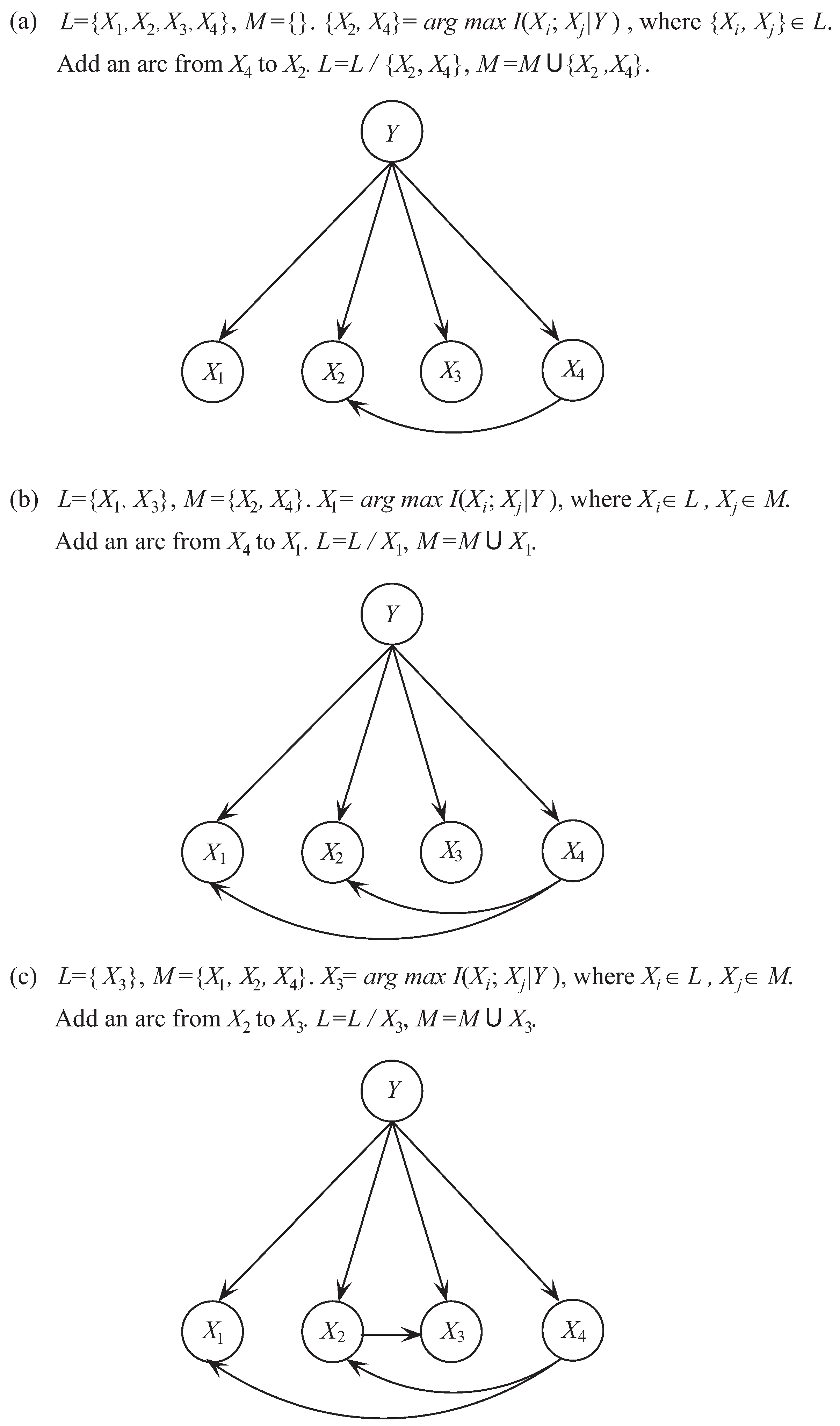
TAN constructs the tree structure by finding a maximum weighted spanning tree [21] (see Figure 1b). The structure is determined by extending Chow-Liu tree [22], which uses CMI to measure the weight of arcs. The CMI between and given the class Y, , is defined as follows [23],
For each attribute , its parent set is . The learning procedure of TAN is shown in Algorithm 1.
Algorithm 1: The Tree-augment Naive Bayes.
To illustrate the learning process of TAN, we take dataset Balance-Scale as an example. Dataset Balance-Scale is from the University of California Irvine (UCI) machine learning repository and has 625 instances, 4 attributes, and 3 class labels. As a 1-dependence BNC, TAN requires that each attribute can have at most 1 parent. In the first step we need to find the most significant dependence between attributes. As shown in Figure 2a, corresponds to the maximum of for any attribute pairs. Then arc is added to the topology of TAN. In the second step, we need to find the next significant dependence relationship between attributes. As shown in Figure 2b, corresponds to the maximum of where and . Then arc is added to the topology. The next iteration begins. As shown in Figure 2c, corresponds to the maximum of where and . Then arc is added to the topology. Finally, there exist at least 1 dependence relationship between any attribute and other attributes and the learning procedure of TAN stops.
According to the structure of TAN, is calculated by
where () represents the parent attribute of (). Correspondingly, can be calculated by
According to Equation (6) and Equation (9), the difference between and can be calculated by
Thus, the difference between and is the summation of 1-order CMIs that correspond to the conditional dependence relationships among attributes. Equation (10) can clarify why TAN applies CMI to fully describe the 1-dependence relationships in the maximum weighted spanning tree. As TAN is a successful structure augmentation of NB, many researchers suggest that identifying significant dependencies can help to achieve more precise classification accuracy [24,25]. Ziebart et al. [26] model the selective forest-augmented naive Bayes by allowing attributes to be optionally dependent on the class. Jing and Pavlovi [27] presented the boosted BNC which greedily builds the structure with the arcs with the highest value of CMI.
KDB [28] extends the network structure further by using variable k to control the attribute dependence spectrum (see Figure 1c). KDB first sorts attributes by comparing MI . Suppose that the attribute order is , is calculated by
where is the set of k parent attributes of when . Whereas when , takes the first attributes in the order as its parent attributes. Correspondingly, can be calculated by
According to Equation (6) and Equation (12), the difference between and can be calculated by
Thus, the difference between and is actually the summation of these CMIs of different orders.
Extending the network structure with high attribute dependence spectrum has become popular to improve the classification performance of BNCs [29]. Pernkopf and Bilmes [30] establish k-graphs via ranking attributes by means of a greedy algorithm and selecting the k best parents by scoring each possibility with the classification accuracy. Lu and Mineichi [31] propose k-dependence classifier chains with label-specific features and demonstrate the effectiveness of the method.
3. Extensive Tree-Augmented Naive Bayes
KDB allows us to construct classifiers at arbitrary points (values of k) along the attribute dependence spectrum. To build an ideal KDB, we need to learn how to maximize the Kullback–Leibler divergence shown in Equation (13). The original KDB sort attributes by comparing MI and uses a set of 1-order CMIs (e.g., ) rather than one higher-order CMI (e.g., ) to measure the conditional dependencies between and its parent attributes. To illustrate the difference between these two measures, we take data set Census-income, which has 299,285 instances, 41 attributes and 2 class labels, for example to learn specific KDB, corresponding distributions of and are shown in Figure 3, where the X-axis denotes the index of attributes sorted in the decreasing order of . From Figure 3, the distribution of differs greatly to that of , thus the former is not appropriate to approximate the latter.
CMI or is a popular measure to evaluate the dependency relationship between attributes, and the maximum weighted spanning tree learned by TAN describes the most significant dependencies in its 1-dependence structure. While may fail to discriminate the dependency relationships given different class labels. The definition of CMI shown in Equation (7) can be represented as follows,
where measures the informational correlation between and given specific class label y and is defined as follows,
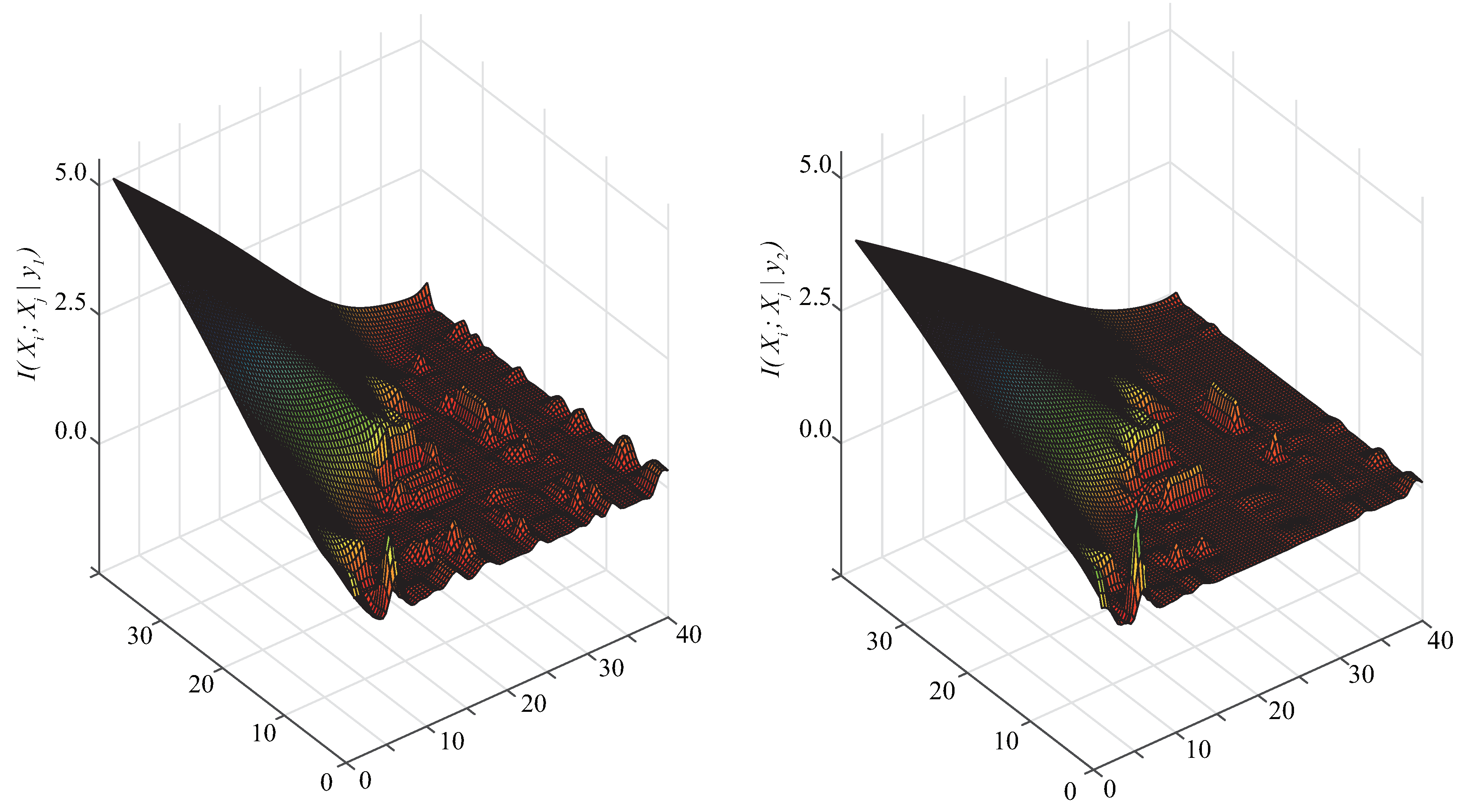
From Equation (1), for restricted BNCs the most important issue is how to deeply mine the significant conditional dependencies among attributes given class label y. Whereas from Equation (14), CMI or is just a simple uniform averaging of , and the latter assumes that the data set has been divided into subsets and each subset corresponds a specific class label. To illustrate the variety of with different class labels, we present their comparison on data set Census-income in Figure 4. As Figure 4 shows, the distribution of differs greatly as y changes. Correspondingly the network structures, in which the conditional dependencies are measured by , should be different.
According to Figure 3 and Figure 4, may not be able to approximate , and to discriminate the conditional dependence between attributes, rather than is appropriate to measure the conditional dependencies implicated in different subspaces of training data. Thus, motivated by the learning schemes of TAN and KDB, the structure of the proposed BNC is just like an extension of TAN from 1-dependence BNC to arbitrary k-dependence BNC, and we respectively learn sub-classifiers from subspaces of training data. The attributes are sorted in such a way that the Kullback–Leibler divergence will be maximized and each attribute can have at most k parent attributes. Supposed that the attribute order is , from the chain rule of joint probability of BNC (see Equation (2)) we know that any possible parents of attribute must be selected from . As a k-dependence BNC, ETAN uses a heuristic search strategy and the learning procedure of ETAN is divided into two parts: when , all attributes in will be selected as the parents of ; when , only k attributes in will be selected as the parents of . The learning procedure of one sub-model of ETAN is shown in Algorithm 2.
Algorithm 2: Sub-ETAN (y,k).
To illustrate the learning process of ETAN, we also take dataset Balance-Scale as an example and set , . In the first step we need to find the most significant dependence between attributes. As shown in Figure 5a, corresponds to the maximum of for any attribute pairs. Then arc is added to the topology of ETAN. In the second step, we need to find the next significant dependence relationship between attributes. As shown in Figure 5b, corresponds to the maximum of where and . Then arcs and are added to the topology. The next iteration begins. As shown in Figure 5c, corresponds to the maximum of where and . Then arcs and are added to the topology. Finally, there exist at least k dependence relationship between any attribute and other attributes and the learning procedure of ETAN stops.
For testing instance , its class label y will correspond to one of the candidate classifiers, whose structure may lead to the maximum of joint probability , i.e., BNC). The prediction procedure of our proposed method, the extensive tree-augmented naive Bayes, is shown in Algorithm 3.
Algorithm 3: The Extensive tree-augmented naive Bayes (ETAN).
4. Experimental Results
We compare the performance of our proposed methods with other algorithms. All experiments are carried out on 40 data sets from UCI machine learning repository. Table 1 shows the details of each data set used, including the number of instances, attributes, and the class. These data sets are arranged in the order of the number of instances. For each data set, numeric attributes are discretized using Minimum Description Length discretization [32]. To allow the proposed algorithm to be compared with Weka’s algorithms, missing values for qualitative attributes are replaced with modes and those for quantitative attributes are replaced with means from the training data.
The following algorithms are compared for experimental study,
In machine learning, zero-one loss is the most common function to measure the classification performance. Kohavi and Wolpert [35] presented a bias-variance decomposition of zero-one loss for analyzing supervised learning scenarios. Bias represents the systematic component of error, which measures how closely the classifier can describe surfaces for a data set. Variance represents the component of error that stems from sampling, which represents the sensitivity of the classifier to changes in training data. The estimation of these measures is using 10-fold cross validation to provide an accurate evaluation of the performance of algorithms. The experimental results of zero-one loss, bias and variance are shown in Table A1–Table A3 respectively in Appendix A. Statistically, we employ win/draw/loss when two algorithms are compared with respect to a performance measure. A win and a draw respectively indicate that the algorithm has significantly and not significantly lower error than the comparator. We assess a difference as significant if the outcome of a one-tailed binomial sign test is less than . Base probability estimates with M-estimation which leads to more accurate probabilities are applied in our paper, where the value of M is 1 [36].
4.1. ETAN vs. BNCs
In this section, we present experimental results of our proposed algorithms, ETAN. Table 2 displays the win/draw/loss records summarizing the relative zero-one loss, bias, and variance of different algorithms. Cell in Table 2 contains win/draw/loss records for the BNC on row i against the BNC on column j.
As shown in Table 2, ETAN respectively performs significantly better than NB on 28 datasets in terms of zero-one loss. In particular, ETAN shows obvious advantages when compared with TAN (19 wins). ETAN has a clear edge over KDB with win/draw/loss records of 17/14/9. Ensemble of classifiers, e.g., AODE and WAODE, brings improvement in accuracy in the sense that small variations in the training set would lead them to produce very different models, which help achieve higher classification accuracy compared to these single-structure classifiers. ETAN is also an ensemble but has higher attribute dependence spectrum than AODE or WAODE. It retains the advantage over AODE and WAODE in terms of zero-one loss, although less significantly. As structure complexity increases, ETAN uses higher-order CMI to measure the high-dependence relationships that may help to improve the classification performance.
The win/draw/loss records of bias and variance are also shown in Table 2. Bias-variance analysis of BNCs is given in the following discussion. By modeling BNCs with respect to the class labels, ETAN makes full use of the training data. For bias, ETAN performs better than NB (32/4/4). When ETAN is compared with 1-dependence classifier, ETAN beats TAN on 17 datasets and loses on 8 datasets. As each sub-model in ETAN is k-dependence classifier, ETAN beats AODE on 20 datasets. It indicates that BNCs with more interdependencies can perform better in terms of bias. Variance-wise, NB performs the best, because the structure of NB is definite and insensitive to variations in training data. For single-structure BNCs, higher-dependence BNCs (e.g., KDB) performs worse than lower-dependence BNCs (e.g., TAN). This also holds for ensemble classifiers, and ETAN performs worse than AODE and WAODE. The reason may be that further dependence discovery will result in overfitting.
ETAN is a structural augmentation of TAN where every attribute takes the class variable and at most k other attributes as its parents. k-order CMI is introduced to measure the conditional dependencies among attributes and the final structure is an extended maximum spanning tree. This alleviates some of NB’s independence assumption and therefore reduces its bias at the expense of increasing its variance. As can be seen from Table 2, ETAN performs better in terms of variance than NB on 4 datasets, i.e., Anneal, Vowel, Dis and Mushrooms. Each dataset has smaller number of instances and larger number of attributes. That may lead to sparsely distributed data and imprecise estimate of probability distribution. For lower quantities of data, the lower variance results in lower error for ETAN, while for larger quantities of data the lower bias results in lower error. ETAN may underfit the sparsely distributed training data that will lead to lower variance and then higher classification accuracy. The ideal datasets on which ETAN has better variance prediction accuracy are those with small data quantity and sparse data. For example, dataset Anneal has only 898 instances but 38 attributes and 6 class labels.
4.2. ETAN vs. Logistic Regression (LR)
In this section, our proposed algorithms are compared with the state-of-the-art algorithm, Logistic Regression (LR). LR can be viewed as a partially parametric approach [37], hence, a BNC can be mapped to a LR model [38]. We use LR’s implementation in Weka, an open source provided by the University of Waikato for machine learning. Weka offers an improved implementation of LR, which use a quasi-Newton to search for the optimized values of attributes and considers the instance weights. The experimental results in terms of zero-one one loss, bias and variance have been shown in the fifth column of Table A1–Table A3 in Appendix A. Table 3 shows the win/draw/loss results. Due to the computational constraints of LR, the size of data sets has an obvious effect on its training time; hence, we have not been able to learn the classification models for the two largest data sets. That is why the sum of the number of all cells is exactly 38.
As we can see from Table 3, ETAN beats LR on 26 data sets, which means ETAN achieves better classification performance than LR. ETAN results in not only better bias performance on 22 data sets but also better variance performance on 21 data sets. In the other words, ETAN is difficult to be beaten by LR.
To further illustrate the advantages of our algorithms, we present the comparison results with respect to zero-one loss in Figure 6, where the X-axis represents the zero-one loss results of ETAN and the Y-axis represents those of LR. Most of the points in Figure 6 are above the diagonal lines, which means that our algorithms have shown better classification performance in general. LR is a popular binary classifier and attempts to predict outcomes based on a set of independent attributes. Among those data sets which correspond to the points under the diagonal lines, most of them have 2 class labels, less than 1000 instances and at least 8 attributes. Obviously, the sparsely distributed data and binary classification may be the main reasons why LR performs better. However, for data sets containing non-binary attributes, ETAN allows us to build (more expressive) non-linear classifiers, which is impossible for LR, unless one “binarizes” all attributes and this may artificially introduce noise.
4.3. Comparison of All Algorithms
To compare multiple algorithms over multiple data sets, Friedman test is used in the following discussion, which ranks the algorithms for each data set [39]. We calculate the rank of each algorithm for each data set separately (assign average ranks in case of tie). The null hypothesis is that there is no significant difference in the average ranks. The Friedman statistic is distributed according to with degrees of freedom. For any level of significance , the null hypothesis will be rejected if . The critical value of for 0.05 with 6 degrees of freedom is 14.07. The Friedman statistic for zero-one loss is 37.90. Therefore, the null hypothesis is rejected.
As the null hypothesis is rejected, we perform Nemenyi test which is used to analyze which pairs of algorithms are significantly different [40]. If the difference between the average ranks of two algorithms is less than the critical difference (CD), their performance is significantly different. For these 7 algorithms and 38 data sets, the value of CD is 1.462.
The comparison of all algorithms against each other with Nemenyi test in terms of zero-one loss is shown in Figure 7. We plot the algorithms on the left line according to average ranks, the higher the position of algorithms, the lower average ranks will be, hence the better performance. As we can see, the rank of ETAN is significantly better than that of other algorithms. WAODE and AODE also achieve lower average rank than KDB, TAN, and NB. It indicates that ensemble classifiers may help to improve performance of the single-structure classifiers. The advantage of ETAN over ADOE and that of KDB over TAN may be attributed to the increasing attribute dependence spectrum.
5. Conclusions
Our work was primarily motivated by the consideration that the structure difference between NB and its variations can be measured by different orders of CMIs in terms of Kullback–Leibler divergence, and conditional dependencies between attributes may vary greatly for different class labels. In this paper, we provide a novel learning algorithm, ETAN, which extends TAN to arbitrary k-dependence BNC. The final network structure is similar to an extended version of maximum weighted spanning tree and corresponds to the maximum of sum of CMIs. ETAN substantially achieves better performance with respect to different evaluation functions and is highly competitive with the state-of-the-art higher-dependence BNC, e.g., KDB.
Author Contributions
All authors have contributed to the study and preparation of the article. Y.L. and L.W. conceived the idea, derived equations and wrote the paper. M.S. did the analysis and finished the programming work. All authors have read and approved the final manuscript.
Funding
This work was supported by the National Natural Science Foundation of China (Grant No. 61272209, 61872164),the Agreement of Science and Technology Development Project, Jilin Province (20150101014JC), and the Fundamental Research Funds for the Central Universities.
Conflicts of Interest
The authors declare no conflict of interest.
Appendix A. Detailed Experimental Results
Table A1.
Experimental results of zero-one loss.
Table A1.
Experimental results of zero-one loss.
Data Set
NB
TAN
KDB
LR
ETAN
AODE
WAODE
Labor
0.0289
0.0211
0.0279
0.0211
0.0274
0.0205
0.0200
Labor-Negotiations
0.0505
0.0763
0.0553
0.0422
0.0237
0.0268
0.0268
Lymphography
0.0902
0.0976
0.1041
0.1422
0.0814
0.0853
0.0951
Iris
0.0590
0.0550
0.0656
0.0343
0.0760
0.0626
0.0624
Hungarian
0.1646
0.1454
0.1480
0.1057
0.1456
0.1597
0.1611
Heart-Disease-C
0.1297
0.1263
0.1299
0.1300
0.1300
0.1171
0.1092
Soybean-Large
0.1070
0.1275
0.1086
0.1104
0.0964
0.0812
0.0655
Ionosphere
0.1220
0.0800
0.0855
0.1117
0.0817
0.0903
0.0061
House-Votes-84
0.0899
0.0410
0.0258
0.0307
0.0406
0.0518
0.0406
Musk1
0.1847
0.1563
0.1535
0.1357
0.1527
0.1670
0.1501
Cylinder-Bands
0.2000
0.3242
0.1939
0.1863
0.1746
0.1684
0.1286
Chess
0.1413
0.1427
0.1119
0.0832
0.1192
0.1380
0.0180
Syncon
0.0516
0.0203
0.0314
0.1123
0.0339
0.0334
0.1827
Balance-Scale
0.1840
0.1843
0.1902
0.0753
0.1877
0.1905
0.0503
Soybean
0.1015
0.0504
0.0491
0.0656
0.0622
0.0690
0.0900
Credit-A
0.0912
0.1171
0.1137
0.1279
0.1266
0.0892
0.0953
Breast-Cancer-W
0.0187
0.0315
0.0449
0.0375
0.0263
0.0243
0.1941
Pima-Ind-Diabetes
0.1957
0.1946
0.1944
0.1898
0.1905
0.1935
0.2398
Vehicle
0.3330
0.2384
0.2494
0.1540
0.2482
0.2435
0.0194
Anneal
0.0354
0.0195
0.0073
0.0788
0.0186
0.0180
0.2104
Vowel
0.3301
0.1931
0.1745
0.1688
0.2135
0.2268
0.1811
Led
0.2322
0.2247
0.2317
0.2211
0.2348
0.2327
0.3766
Car
0.0937
0.0478
0.0387
0.0536
0.0524
0.0597
0.0633
Hypothyroid
0.0116
0.0105
0.0096
0.0181
0.0095
0.0094
0.0315
Dis
0.0165
0.0194
0.0191
0.0195
0.0194
0.0163
0.0078
Sick
0.0246
0.0208
0.0198
0.0277
0.0215
0.0221
0.3212
Abalone
0.4180
0.3134
0.3033
0.3613
0.3089
0.3201
0.0574
Spambase
0.0929
0.0571
0.0497
0.0560
0.0488
0.0631
0.1184
Waveform-5000
0.1762
0.1232
0.1157
0.1207
0.1122
0.1233
0.2172
Page-Blocks
0.0451
0.0306
0.0280
0.0282
0.0259
0.0259
0.0224
Optdigits
0.0685
0.0275
0.0250
0.0382
0.0182
0.0203
0.0902
Satellite
0.1746
0.0948
0.0808
0.1064
0.0834
0.0889
0.0002
Mushrooms
0.0237
0.0001
0.0001
0.0000
0.0001
0.0004
0.0561
Thyroid
0.0994
0.0572
0.0553
0.0999
0.0535
0.0658
0.0561
Letter-Recog
0.2207
0.1032
0.1387
0.1945
0.0569
0.0806
0.0892
Adult
0.1649
0.1312
0.1220
0.1394
0.1215
0.1440
0.0006
Connect-4
0.2660
0.2253
0.2022
0.2279
0.1981
0.2279
0.0158
Waveform
0.0219
0.0152
0.0210
0.0267
0.0140
0.0157
0.3068
Census-Income
0.2303
0.0544
0.0421
-
0.0450
0.0859
0.2083
Poker-Hand
0.4979
0.2865
0.1326
-
0.4040
0.4217
0.1716
Table A2.
Experimental results of Bias.
Table A2.
Experimental results of Bias.
Data Set
NB
TAN
KDB
LR
ETAN
AODE
WAODE
Labor
0.0289
0.0211
0.0279
0.0211
0.0274
0.0205
0.0200
Labor-Negotiations
0.0505
0.0763
0.0553
0.0422
0.0237
0.0268
0.0268
Lymphography
0.0902
0.0976
0.1041
0.1422
0.0814
0.0853
0.0951
Iris
0.0590
0.0550
0.0656
0.0343
0.0760
0.0626
0.0624
Hungarian
0.1646
0.1454
0.1480
0.1057
0.1456
0.1597
0.1611
Heart-Disease-C
0.1297
0.1263
0.1299
0.1300
0.1300
0.1171
0.1092
Soybean-Large
0.1070
0.1275
0.1086
0.1104
0.0964
0.0812
0.0655
Ionosphere
0.1220
0.0800
0.0855
0.1117
0.0817
0.0903
0.0061
House-Votes-84
0.0899
0.0410
0.0258
0.0307
0.0406
0.0518
0.0406
Musk1
0.1847
0.1563
0.1535
0.1357
0.1527
0.1670
0.1501
Cylinder-Bands
0.2000
0.3242
0.1939
0.1863
0.1746
0.1684
0.1286
Chess
0.1413
0.1427
0.1119
0.0832
0.1192
0.1380
0.0180
Syncon
0.0516
0.0203
0.0314
0.1123
0.0339
0.0334
0.1827
Balance-Scale
0.1840
0.1843
0.1902
0.0753
0.1877
0.1905
0.0503
Soybean
0.1015
0.0504
0.0491
0.0656
0.0622
0.0690
0.0900
Credit-A
0.0912
0.1171
0.1137
0.1279
0.1266
0.0892
0.0953
Breast-Cancer-W
0.0187
0.0315
0.0449
0.0375
0.0263
0.0243
0.1941
Pima-Ind-Diabetes
0.1957
0.1946
0.1944
0.1898
0.1905
0.1935
0.2398
Vehicle
0.3330
0.2384
0.2494
0.1540
0.2482
0.2435
0.0194
Anneal
0.0354
0.0195
0.0073
0.0788
0.0186
0.0180
0.2104
Vowel
0.3301
0.1931
0.1745
0.1688
0.2135
0.2268
0.1811
Led
0.2322
0.2247
0.2317
0.2211
0.2348
0.2327
0.3766
Car
0.0937
0.0478
0.0387
0.0536
0.0524
0.0597
0.0633
Hypothyroid
0.0116
0.0105
0.0096
0.0181
0.0095
0.0094
0.0315
Dis
0.0165
0.0194
0.0191
0.0195
0.0194
0.0163
0.0078
Sick
0.0246
0.0208
0.0198
0.0277
0.0215
0.0221
0.3212
Abalone
0.4180
0.3134
0.3033
0.3613
0.3089
0.3201
0.0574
Spambase
0.0929
0.0571
0.0497
0.0560
0.0488
0.0631
0.1184
Waveform-5000
0.1762
0.1232
0.1157
0.1207
0.1122
0.1233
0.2172
Page-Blocks
0.0451
0.0306
0.0280
0.0282
0.0259
0.0259
0.0224
Optdigits
0.0685
0.0275
0.0250
0.0382
0.0182
0.0203
0.0902
Satellite
0.1746
0.0948
0.0808
0.1064
0.0834
0.0889
0.0002
Mushrooms
0.0237
0.0001
0.0001
0.0000
0.0001
0.0004
0.0561
Thyroid
0.0994
0.0572
0.0553
0.0999
0.0535
0.0658
0.0561
Letter-Recog
0.2207
0.1032
0.1387
0.1945
0.0569
0.0806
0.0892
Adult
0.1649
0.1312
0.1220
0.1394
0.1215
0.1440
0.0006
Connect-4
0.2660
0.2253
0.2022
0.2279
0.1981
0.2279
0.0158
Waveform
0.0219
0.0152
0.0210
0.0267
0.0140
0.0157
0.3068
Census-Income
0.2303
0.0544
0.0421
-
0.0450
0.0859
0.2083
Poker-Hand
0.4979
0.2865
0.1326
-
0.4040
0.4217
0.1716
Table A3.
Experimental results of Variance.
Table A3.
Experimental results of Variance.
Data Set
NB
TAN
KDB
LR
ETAN
AODE
WAODE
Labor
0.0395
0.0632
0.0721
0.0328
0.0779
0.0268
0.0221
Labor-Negotiations
0.0653
0.1395
0.1289
0.0655
0.0868
0.0626
0.0626
Lymphography
0.0343
0.1106
0.1408
0.1212
0.0961
0.0412
0.0478
Iris
0.0390
0.0510
0.0364
0.0327
0.0460
0.0394
0.0396
Hungarian
0.0201
0.0556
0.0561
0.0751
0.0411
0.0270
0.0317
Heart-Disease-C
0.0248
0.0479
0.0582
0.0920
0.0591
0.0304
0.0383
Soybean-Large
0.0783
0.1127
0.0982
0.1542
0.0899
0.0747
0.0855
Ionosphere
0.0242
0.0414
0.0581
0.0946
0.0448
0.0319
0.0242
House-Votes-84
0.0066
0.0170
0.0197
0.0714
0.0083
0.0068
0.0123
Musk1
0.1108
0.1191
0.1320
0.1691
0.1157
0.1153
0.1010
Cylinder-Bands
0.0656
0.0724
0.0750
0.1437
0.0888
0.0827
0.0364
Chess
0.0401
0.0491
0.0531
0.0791
0.0578
0.0385
0.0230
Syncon
0.0204
0.0222
0.0301
0.1764
0.0246
0.0161
0.0913
Balance-Scale
0.0848
0.0941
0.0872
0.0339
0.0863
0.0854
0.0334
Soybean
0.0302
0.0593
0.0439
0.0839
0.0395
0.0288
0.0321
Credit-A
0.0249
0.0555
0.0768
0.0737
0.0673
0.0269
0.0264
Breast-Cancer-W
0.0010
0.0372
0.0504
0.0395
0.0376
0.0118
0.0700
Pima-Ind-Diabetes
0.0715
0.0663
0.0689
0.0425
0.0697
0.0729
0.1276
Vehicle
0.1120
0.1297
0.1283
0.0797
0.1330
0.1246
0.0161
Anneal
0.0168
0.0156
0.0152
0.0593
0.0139
0.0118
0.0604
Vowel
0.2542
0.2466
0.2325
0.2239
0.2310
0.2465
0.2489
Led
0.0333
0.0536
0.0565
0.0640
0.0460
0.0372
0.1106
Car
0.0520
0.0375
0.0434
0.0385
0.0427
0.0431
0.0509
Hypothyroid
0.0031
0.0029
0.0024
0.0062
0.0039
0.0026
0.0083
Dis
0.0069
0.0006
0.0011
0.0038
0.0009
0.0048
0.0056
Sick
0.0047
0.0052
0.0043
0.0084
0.0063
0.0038
0.1543
Abalone
0.0682
0.1690
0.1769
0.0746
0.1679
0.1536
0.0111
Spambase
0.0092
0.0157
0.0214
0.0243
0.0177
0.0098
0.0420
Waveform-5000
0.0259
0.0687
0.0843
0.0310
0.0693
0.0403
0.1311
Page-Blocks
0.0135
0.0144
0.0177
0.0123
0.0139
0.0111
0.0137
Optdigits
0.0153
0.0185
0.0254
0.0752
0.0162
0.0133
0.0364
Satellite
0.0139
0.0368
0.0455
0.0517
0.0395
0.0325
0.0001
Mushrooms
0.0043
0.0002
0.0002
0.0001
0.0001
0.0001
0.0239
Thyroid
0.0205
0.0252
0.0272
0.0453
0.0239
0.0202
0.0241
Letter-Recog
0.0471
0.0591
0.0113
0.0422
0.0523
0.0709
0.0417
Adult
0.0069
0.0165
0.0285
0.0108
0.0236
0.0104
0.0004
Connect-4
0.0156
0.0149
0.0309
0.0127
0.0373
0.0199
0.0023
Waveform
0.0009
0.0053
0.0037
0.0024
0.0059
0.0023
0.0632
Census-Income
0.0052
0.0100
0.0110
-
0.0144
0.0138
0.0224
Poker-Hand
0.0000
0.0424
0.0633
-
0.0440
0.0273
0.0602
References
Acid, S.; Campos, L.M.; Castellano, J.G. Learning Bayesian network classifiers: Searching in a space of partially directed acyclic graphs. Mach. Learn.2005, 59, 213–235. [Google Scholar] [CrossRef]
Hand, D.J.; Yu, K. Idiot’s Bayes not so stupid after all? Int. Stat. Rev.2001, 69, 385–398. [Google Scholar]
Kontkanen, P.; Myllymaki, P.; Silander, T.; Tirri, H. BAYDA: Software for Bayesian classification and feature selection. In Proceedings of the 4th International Conference on Knowledge Discovery and Data Mining (KDD-1998); AAAI Press: Menlo Park, CA, USA, 1998; pp. 254–258. [Google Scholar]
Langley, P.; Sage, S. Induction of selective Bayesian classifiers. In Uncertainty Proceedings 1994; Morgan Kaufmann: Burlington, MA, USA, 1994; pp. 399–406. [Google Scholar]
Ekdahl, M.; Koski, T. Bounds for the loss in probability of correct classification under model based approximation. J. Mach. Learn. Res.2006, 7, 2449–2480. [Google Scholar]
Yang, Y.; Webb, G.I.; Cerquides, J. To select or to weigh: A comparative study of linear combination schemes for superparent-one-dependence estimators. IEEE Trans. Knowl. Data Eng.2007, 19, 1652–1665. [Google Scholar] [CrossRef]
Pernkopf, F.; Wohlmayr, M. Stochastic margin-based structure learning of Bayesian network classifiers. Pattern Recognit.2013, 46, 464–471. [Google Scholar] [CrossRef] [PubMed]
Xiao, J.; He, C.; Jiang, X. Structure identification of Bayesian classifiers based on GMDH. Knowl. Based Syst.2009, 22, 461–470. [Google Scholar] [CrossRef]
Louzada, F.; Ara, A. Bagging k-dependence probabilistic networks: An alternative powerful fraud detection tool. Expert Syst. Appl.2012, 39, 11583–11592. [Google Scholar] [CrossRef]
Pazzani, M.; Billsus, D. Learning and revising user profiles: The identification of interesting web sites. Mach. Learn.1997, 27, 313–331. [Google Scholar] [CrossRef]
Hall, M.A. Correlation-Based Feature Selection for Machine Learning. Ph.D. Thesis, University of Waikato, Hamilton, New Zealand, 1999. [Google Scholar]
Jiang, L.X.; Cai, Z.H.; Wang, D.H.; Zhang, H. Improving tree augmented naive bayes for class probability estimation. Knowl. Based Syst.2012, 26, 239–245. [Google Scholar] [CrossRef]
Grossman, D.; Domingos, P. Learning Bayesian network classifiers by maximizing conditional likelihood. In International Conference on Machine Learning; ACM: Hyères, France, 2004. [Google Scholar]
Ruz, G.A.; Pham, D.T. Building Bayesian network classifiers through a Bayesian complexity monitoring system. Proc. Inst. Mech. Eng. Part C J. Mech. Eng. Sci.2009, 223, 743–755. [Google Scholar] [CrossRef]
Pearl, J. Probabilistic Reasoning in Intelligent Systems: Networks of Plausible Inference; Morgan Kaufmann: San Francisco, CA, USA, 1988. [Google Scholar]
Jingguo, D.; Jia, R.; Wencai, D. An improved evolutionary approach-based hybrid algorithm for Bayesian network structure learning in dynamic constrained search space. In Neural Computing and Applications; Springer: Berlin, Germany, 2018; pp. 1–22. [Google Scholar]
Jiang, L.; Zhang, L.; Li, C.; Wu, J. A Correlation-based feature weighting filter for naive bayes. IEEE Trans. Knowl. Data Eng.2019, 31, 201–213. [Google Scholar] [CrossRef]
Jiang, L.; Li, C.; Wang, S.; Zhang, L. Deep feature weighting for naive bayes and its application to text classification. Eng. Appl. Artif. Intell.2016, 52, 26–39. [Google Scholar] [CrossRef]
Zhao, Y.; Chen, Y.; Tu, K. Learning Bayesian network structures under incremental construction curricula. Neurocomputing2017, 258, 30–40. [Google Scholar] [CrossRef]
Wu, J.; Cai, Z. A naive Bayes probability estimation model based on self-adaptive differential evolution. J. Intell. Inf. Syst.2014, 42, 671–694. [Google Scholar] [CrossRef]
Friedman, N.; Dan, G.; Goldszmidt, M. Bayesian network classifiers. Mach. Learn.1997, 29, 131–163. [Google Scholar] [CrossRef]
Shannon, C.E.; Weaver, W. The mathematical theory of communication. Bell Labs Tech. J.1950, 3, 31–32. [Google Scholar] [CrossRef]
Bielza, C. Discrete Bayesian network classifiers: A survey. ACM Comput. Surv. (CSUR)2014, 47, 1–43. [Google Scholar] [CrossRef]
Francois, P.; Wray, B.; Webb, G.I. Accurate parameter estimation for Bayesian network classifiers using hierarchical Dirichlet processes. Mach. Learn.2018, 107, 1303–1331. [Google Scholar]
Ziebart, B.D.; Dey, A.K.; Bagnell, J.A. Learning selectively conditioned forest structures with applications to DBNs and classification. In Proceedings of the 23rd Conference Annual Conference on Uncertainty in Artificial Intelligence; AUAI Press: Corvallis, OR, USA, 2007; pp. 458–465. [Google Scholar]
Sahami, M. Learning limited dependence Bayesian classifiers. In Proceedings of the Second International Conference on Knowledge Discovery and Data Mining; AAAI: Menlo Park, CA, USA, 1996; pp. 335–338. [Google Scholar]
Luo, L.; Yang, J.; Zhang, B. Nonparametric Bayesian correlated group regression with applications to image classification. IEEE Trans. Neural Netw. Learn. Syst.2018, 99, 1–15. [Google Scholar] [CrossRef] [PubMed]
Pernkopf, F.; Bilmes, J.A. Efficient heuristics for discriminative structure learning of Bayesian network classifiers. J. Mach. Learn. Res.2010, 11, 2323–2360. [Google Scholar]
Sun, L.; Kudo, M. Optimization of classifier chains via conditional likelihood maximization. Pattern Recognit.2018, 74, 503–517. [Google Scholar] [CrossRef]
Fayyad, U.M.; Irani, K.B. Multi-interval discretization of continuous valued attributes for classification learning. In Proceedings of the 5th International Joint Conference on Artificial Intelligence; Organ Kaufmann Publishers Inc.: San Francisco, CA, USA, 1993; pp. 1022–1029. [Google Scholar]
Webb, G.I.; Boughton, J.R.; Wang, Z. Not so naive Bayes: Aggregating one-dependence estimators. Mach. Learn.2005, 58, 5–24. [Google Scholar] [CrossRef]
Jiang, L.; Zhang, H. Weightily averaged one-dependence estimators. In Proceedings of the 9th Biennial Pacific Rim International Conference on Artificial Intelligence; Springer: Berlin, Germany, 2006; pp. 970–974. [Google Scholar]
Kohavi, R.; Wolpert, D. Bias plus variance decomposition for zero-one loss functions. In Proceedings of the Thirteenth International Conference on Machine Learning; organ Kaufmann Publishers Inc.: San Francisco, CA, USA, 1996; pp. 275–283. [Google Scholar]
Cestnil, B. Estimating probabilities: A crucial task in machine learning. Proc. Ninth Eur. Conf. Artif. Intell.1990, 6–10, 147–149. [Google Scholar]
McLachlan, G. Discriminant Analysis and Statistical Pattern Recognition; John Wiley & Sons: Hoboken, NJ, USA, 2004. [Google Scholar]
Roos, T.; Wettig, H.; Grunwald, P. On discriminative Bayesian network classifiers and logistic regression. Mach. Learn.2005, 59, 267–296. [Google Scholar] [CrossRef]
Demisar, J.; Schuurmans, D. Statistical comparisons of classifiers over multiple data sets. J. Mach. Learn. Res.2006, 7, 1–30. [Google Scholar]
Nemenyi, P. Distribution-Free Multiple Comparisons. Ph.D. Thesis, Princeton University, Princenton, NJ, USA, 1963. [Google Scholar]
Figure 1.
Examples of different BNCs. (a) Naive Bayes, (b) Tree-augmented naive Bayes, (c) k-dependence Bayesian Classifier.
Figure 1.
Examples of different BNCs. (a) Naive Bayes, (b) Tree-augmented naive Bayes, (c) k-dependence Bayesian Classifier.
Figure 2.
The learning procedure of TAN on Balance-Scale.
Figure 2.
The learning procedure of TAN on Balance-Scale.
Figure 3.
Distributions of and on Census-income.
Figure 3.
Distributions of and on Census-income.
Figure 4.
with different class labels on Census-income.
Figure 4.
with different class labels on Census-income.
Figure 5.
The learning procedure of ETAN with k = 2 on Balance-Scale.
Figure 5.
The learning procedure of ETAN with k = 2 on Balance-Scale.
Figure 6.
Comparison between LR and ETAN in terms of zero-one loss.
Figure 6.
Comparison between LR and ETAN in terms of zero-one loss.
Figure 7.
Nemenyi test for all algorithms.
Figure 7.
Nemenyi test for all algorithms.
Table 1.
Data sets.
Table 1.
Data sets.
No.
Data Set
Ins.
Att.
Class
No.
Data Set
Inst.
Att.
Class
1
Labor
57
16
2
21
Vowel
990
13
11
2
Labor-Negotiations
57
16
2
22
Led
1000
7
10
3
Lymphography
150
4
3
23
Car
1728
6
4
4
Iris
150
4
3
24
Hypothyroid
3163
25
2
5
Hungarian
294
13
2
25
Dis
3772
29
2
6
Heart-Disease-C
303
13
2
26
Sick
3772
29
2
7
Soybean-Large
307
35
19
27
Abalone
4177
8
3
8
Ionosphere
351
34
2
28
Spambase
4601
57
2
9
House-Votes-84
435
16
2
29
Waveform-5000
5000
40
3
10
Musk1
476
166
2
30
Page-Blocks
5473
10
5
11
Cylinder-Bands
540
39
2
31
Optdigits
5620
64
10
12
Chess
551
39
2
32
Satellite
6435
36
6
13
Syncon
600
60
6
33
Mushrooms
8124
22
2
14
Balance-Scale
625
4
3
34
Thyroid
9169
29
20
15
Soybean
683
35
19
35
Letter-Recog
20000
26
2
16
Credit-A
690
15
2
36
Adult
48842
14
2
17
Breast-Cancer-W
699
9
2
37
Connect-4
67557
42
3
18
Pima-Ind-Diabetes
768
8
2
38
Waveform
100000
21
3
19
Vehicle
846
18
4
39
Census-Income
299285
41
2
20
Anneal
898
38
6
40
Poker-Hand
1025010
10
10
Table 2.
The records of win/draw/loss for BNCs and our algorithms.
Table 2.
The records of win/draw/loss for BNCs and our algorithms.
BNC
NB
TAN
KDB
AODE
WAODE
TAN
27/5/8
-
-
-
-
KDB
25/10/5
16/13/11
-
-
-
Zero-one loss
AODE
29/8/3
13/15/12
13/14/13
-
-
WAODE
28/7/5
19/14/7
18/13/9
14/19/7
-
ETAN
30/6/4
21/11/8
19/12/9
18/13/9
15/15/10
TAN
28/5/7
-
-
-
-
KDB
26/8/6
18/14/8
-
-
-
Bias
AODE
31/7/2
14/10/16
13/6/21
-
-
WAODE
24/2/14
19/4/17
18/4/18
18/4/18
-
ETAN
32/4/4
18/14/8
9/19/12
20/13/7
19/3/18
TAN
6/2/32
-
-
-
-
KDB
9/2/29
10/7/23
-
-
-
Variance
AODE
10/11/19
30/3/7
29/3/8
-
-
WAODE
12/5/22
21/3/16
21/1/18
12/4/24
-
ETAN
4/5/31
15/8/17
24/6/10
3/6/31
18/3/19
Table 3.
The records of win/draw/loss for LR and our algorithms.
Table 3.
The records of win/draw/loss for LR and our algorithms.


