Article

Mesoscopic Simulation of the (2 + 1)-Dimensional Wave Equation with Nonlinear Damping and Source Terms Using the Lattice Boltzmann BGK Model

1
College of Mathematics and Informatics, FJKLMAA, Fujian Normal University, Fuzhou 350117, China
2
School of Mathematics and Statistics, Huazhong University of Science and Technology, Wuhan 430074, China
*
Author to whom correspondence should be addressed.
Entropy 2019, 21(4), 390; https://doi.org/10.3390/e21040390
Submission received: 13 March 2019 / Revised: 3 April 2019 / Accepted: 9 April 2019 / Published: 11 April 2019
(This article belongs to the Special Issue Thermodynamics of Non-Equilibrium Gas Flows)

Abstract

:
In this work, we develop a mesoscopic lattice Boltzmann Bhatnagar-Gross-Krook (BGK) model to solve (2 + 1)-dimensional wave equation with the nonlinear damping and source terms. Through the Chapman-Enskog multiscale expansion, the macroscopic governing evolution equation can be obtained accurately by choosing appropriate local equilibrium distribution functions. We validate the present mesoscopic model by some related issues where the exact solution is known. It turned out that the numerical solution is in very good agreement with exact one, which shows that the present mesoscopic model is pretty valid, and can be used to solve more similar nonlinear wave equations with nonlinear damping and source terms, and predict and enrich the internal mechanism of nonlinearity and complexity in nonlinear dynamic phenomenon.

1. Introduction

Nonlinear dynamic phenomenon, which exists in many fields of science and engineering, such as hydrodynamic, nonlinear optics, biology, plasma physics, and so on, can be modeled by many systems of nonlinear partial differential equations (NPDEs) [1,2]. The dynamical processes of these nonlinear systems are very important for both production and scientific research, and they should be studied by a suitable method designed to treat the nonlinear problems. Many researchers use different analytical or numerical methods to investigate various nonlinear dynamic systems. Because of the complexity and particularity of the nonlinear evolution equations, there is no unity approach to find every solution to the nonlinear dynamic systems. Consequently, how to construct accurate and available methods to solve the nonlinear evolution equations has been an absorbing research career. In recent decades, with the vigorous development of computer science and technology, researchers have developed many different types of numerical methods to obtain numerical solutions, including the finite element, finite difference, finite volume, variational iteration, and spectral methods, etc. [3].
In this work, the generalized (2 + 1)-dimensional dynamical equation with nonlinear damping and source terms is considered to be as follows:
2 u t 2 + α u t = β Δ u + f ( x , y , t , u ) , ( x , y ) Ω , t [ t 0 , T ] ,
where Ω = { ( x , y ) : a x b , c y d } . The initial conditions associated with Equation (1) are given as follows:
u ( x , y , t 0 ) = φ 1 ( x , y ) , ( x , y ) Ω u t ( x , y , t 0 ) = φ 2 ( x , y ) , ( x , y ) Ω ,
and the Dirichlet boundary conditions are given by
u ( a , y , t ) = ϕ 1 ( y , t ) , t [ t 0 , T ] , u ( b , y , t ) = ϕ 2 ( y , t ) , t [ t 0 , T ] , u ( x , c , t ) = ϕ 3 ( x , t ) , t [ t 0 , T ] , u ( x , d , t ) = ϕ 4 ( x , t ) , t [ t 0 , T ] ,
where u ( x , y , t ) is the scalar variable; t is the time; Δ is the Laplace operator; the parameter α , β are supposed to be real number with α , β 0 . α is the alleged dissipative term. When α = 0 , Equation (1) is degraded into the undamped wave equation, while α > 0 , to the damped one. The known functions φ 1 ( x , y ) and φ 2 ( x , y ) represent wave kinks or modes and velocity, respectively. and ϕ i , ( i = 1 4 ) are known functions of their arguments. In recent years, many scholars used different types of methods to obtain the numerical solution, such as the implicit Lie-group iterative scheme [4], the meshless method [5], the space-time spectral method [6], the compact finite difference method [7], the nonconforming quadrilateral finite element method [8].
Recently, the mesoscopic lattice Boltzmann method (LBM) has made significant progress in the research nonlinear dynamical equations and evolving process of complexity micro-mesoscopic systems [9], especially in fluid mechanics [10,11,12]. Unlike traditional macroscopic numerical methods, which are independent of the discrete macroscopic evolution equations, the LBM is based on the mesoscopic kinetic evolution equations with distribution functions when the expression of the equilibrium distribution function is known. The fundamental idea is to take the place of the differential evolution equations of nonlinear system by the discrete kinetic Boltzmann equations. To obtain the macroscopic fluid behavior, we just need to calculate the discrete Boltzmann equations to obtain the evolution of the distribution function. From a computational resource perspective, the remarkable merits are brevity of programming, numerical potency, inherent parallelism, and ease treatment of intricate boundary conditions. This kind of method has comprehensive capacities in quite several fields, from phonon transport [13] to approximate incompressible flows [14,15,16,17,18,19,20,21,22,23,24,25], full compressible flows [26,27,28,29,30,31,32,33,34,35,36,37], dendrite growth [38,39] and thermal multiphase flows [40]. Recently, the mesoscopic kinetics method is also becoming increasingly popular in computational mathematics and engineering science for solving certain NPDEs, including Burgers’ equations [41,42], Korteweg-de Vries equation [43], Gross-Pitaevskii equation [44], convection-diffusion equation [45,46,47,48,49,50,51], Kuramoto-Sivashinsky equation [52], wave equation [53,54], Dirac equation [55], Poisson equation [56] etc.
Inspired by the successful promotion and application of the mesoscopic LBM in modeling nonlinear convection-diffusion system [45,46], the aim of this work is to further develop and apply the lattice Boltzmann Bhatnagar-Gross-Krook (BGK) method to solve (2 + 1)-dimensional wave equation with nonlinear damping and source terms. In the process of linking the mesoscopic Boltzmann equation to the nonlinear damped evolution system, we should choose suitable local equilibrium distribution functions to meet some constraints.
The content of this work is as follows: the next section presents the mesoscopic Boltzmann BGK model and deduces the wave equation with nonlinear damping and source terms through the multiscale expansion technique. Numerical verification of the model is presented in Section 3. Finally, a summary of the research is given in the last section.

2. Lattice Boltzmann BGK Model

In the present lattice Boltzmann BGK model, we use a single relaxation factor model for collision terms in this work. The discrete Boltzmann equation of the model with the BGK model takes the form [45]
f j ( x + c j Δ t , t + Δ t ) = f j ( x , t ) 1 τ f j ( x , t ) f j e q ( x , t ) + Δ t F j ( x , t ) + Δ t 2 2 F j ( x , t ) t ,
where τ is the dimensionless relaxation time which regulates the rate of access to equilibrium state, f j ( x , t ) and f j e q ( x , t ) are the distribution function and local equilibrium distribution function, respectively, and F j ( x , t ) is the distribution function for the source term. { c j , j = 0 , 1 , , 8 } is the collection of discrete directions of the particle velocity, for D 2 Q 9 model, { c j , j = 0 , 1 , , 8 } = { ( 0 , 0 ) , ( ± c , 0 ) , ( 0 , ± c ) , ( ± c , ± c ) } , c = Δ x / Δ t , Δ x is the spatial step, Δ t is the time step.
In contrast to the common Lattice BGK model, we define the first derivative of u ( x , t ) as the following conservation condition [53]
u t = j f j ( x , t ) = j f j e q ( x , t ) .
To obtain the corresponding macroscopic evolution equation exactly, we should take f j e q as
f j e q = w j u t + c s 2 ( u u t ) I : ( c j c j c s 2 I ) 2 c s 4 ,
where the item I is the unit tensor, the item c s is referring to the sound speed, satisfy c s 2 = c 2 / 3 . w j are the weights coefficients and satisfy the following conditions: j w j = 1 , j w j c j = 0 , j w j c j c j = c s 2 I , then w 0 = 4 / 9 , w 1 4 = 1 / 9 , w 5 , 8 = 1 / 36 .
Meanwhile, the corresponding source term F j is taken as
F j = w j F ,
where
F = f ( x , t , u ) α u t .
Then, f j e q and F j should satisfy the following conservation conditions:
j c j f j e q = 0 , j c j c j f j e q = c s 2 u I , j F j = F , j c j F j = 0 ,
To obtain the macroscopic evolution Equation (1), we apply the Chapman-Enskog multiscale expansion to the distribution function, the first order time derivative, the spatial derivative and the source term as follows:
f j = f j e q + ε f j ( 1 ) + ε 2 f j ( 2 ) , t = ε t 1 + ε 2 t 2 , = ε 1 , F = ε F ( 1 ) ,
where the item ε is as a small Knudsen number. Then, from Equation (7), and according to Equation (8), we obtain
j f j ( k ) = 0 ( k 1 ) , j F j ( 1 ) = F ( 1 ) , j c j F j ( 1 ) = 0 ,
where F j ( 1 ) = w j F ( 1 ) .
Employing the Taylor formula to discrete Boltzmann Equation (2) at point ( x ,t), we have
D j f j + Δ t 2 D j 2 f j + = 1 τ Δ t ( f j f j e q ) + F j + Δ t 2 F j t ,
where D j = t + c j · . Substitute Equation (10) into Equation (12), we have
ε D 1 j + ε 2 t 2 ( f j e q + ε f j ( 1 ) ) + Δ t 2 ε D 1 j + ε 2 t 2 2 f j e q + = 1 τ Δ t ( ε f j ( 1 ) + ε 2 f j ( 2 ) ) + ε F j ( 1 ) + ε 2 Δ t 2 F j ( 1 ) t 1 ,
where D 1 j = t 1 + c j · 1 .
Then we derive the first- and second-order equation in ε as
O ( ε 1 ) : D 1 j f j e q = 1 τ Δ t f j ( 1 ) + F j ( 1 ) ,
O ( ε 2 ) : f j e q t 2 + D 1 j f j ( 1 ) + Δ t 2 D 1 j 2 f j e q = 1 τ Δ t f j ( 2 ) + Δ t 2 F j ( 1 ) t 1 .
Multiplying both sides of Equation (14) by the operator D 1 j , we obtain
D 1 j 2 f j e q = 1 τ Δ t D 1 j f j ( 1 ) + D 1 j F j ( 1 ) ,
then substitute Equation (16) into Equation (15), we get
f j e q t 2 + 1 1 2 τ D 1 j f j ( 1 ) + Δ t 2 c j · 1 F j ( 1 ) = 1 τ Δ t f j ( 2 ) .
Summing Equations (14) and (17) over i and using Equations (5), (9) and (11), we get
2 u t 1 t = F ( 1 ) ,
2 u t 2 t + 1 1 2 τ 1 · j c j f j ( 1 ) = 0 .
Based on Equation (14), and using Equations (9) and (11), we have
j c j f j ( 1 ) = τ Δ t j c j ( D 1 j f j e q F j ( 1 ) ) = τ Δ t t 1 j c j f j e q + 1 · j c j c j f j e q j c j F j ( 1 ) = τ Δ t c s 2 1 u .
Then, substituting Equation (20) into Equation (19), we obtain
2 u t 2 t τ Δ t c s 2 1 1 2 τ 1 · 1 u = 0 .
Therefore, when Equation (18) × ε + Equation (21) × ε 2 is applied, we have
2 u t 2 τ Δ t c s 2 1 1 2 τ Δ u = F .
To recover Equation (1) to order O ( ε 2 ) , we only need to let
β = τ Δ t c s 2 1 1 2 τ , F = f ( x , y , t , u ) α u t .
so, we have
τ = 1 2 + β Δ t c s 2 .
In the calculation process, to get u ( x , t ) , using Equation (5), and applying the difference scheme to the item u ( x , t ) t , we have
j f j ( x , t ) = u ( x , t ) t = u ( x , t ) u ( x , t Δ t ) Δ t ,
then we get
u ( x , t ) = Δ t j f j ( x , t ) + u ( x , t Δ t ) .

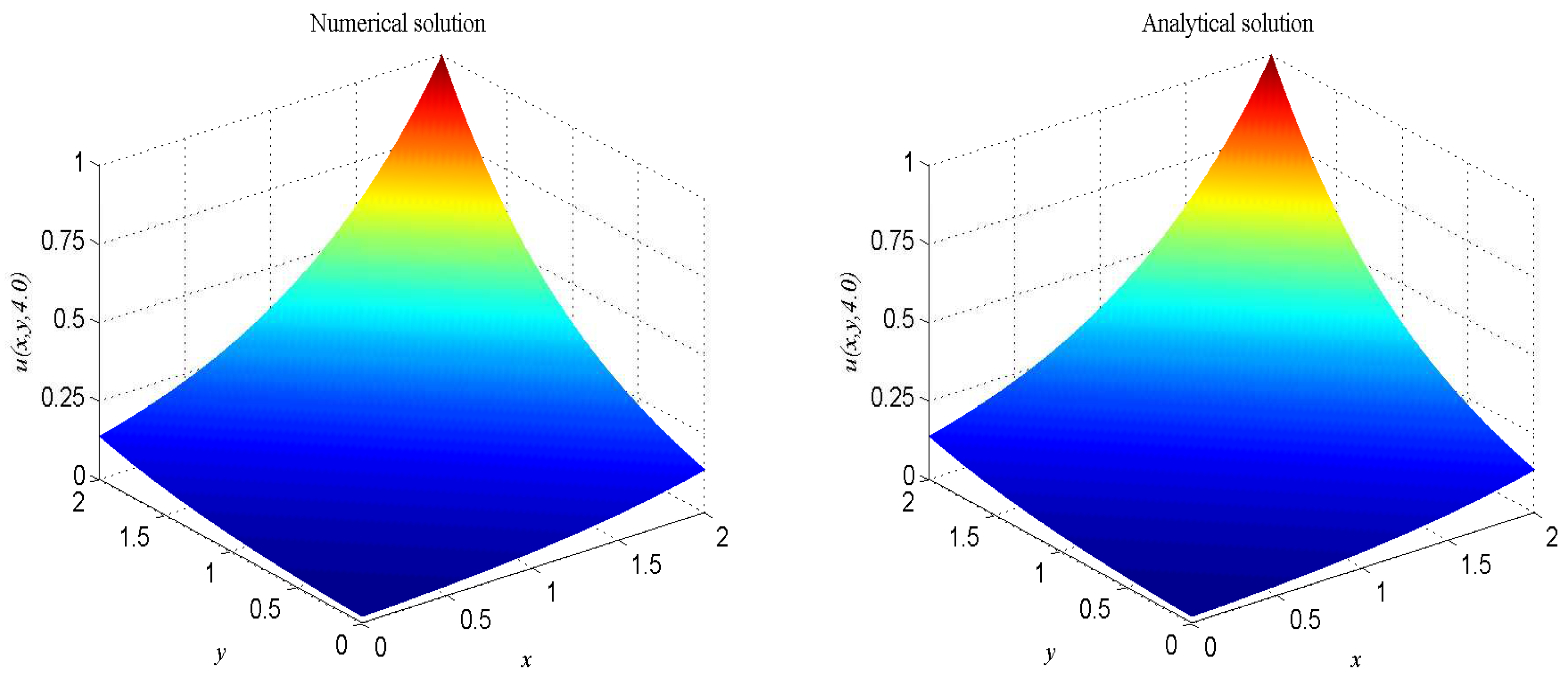
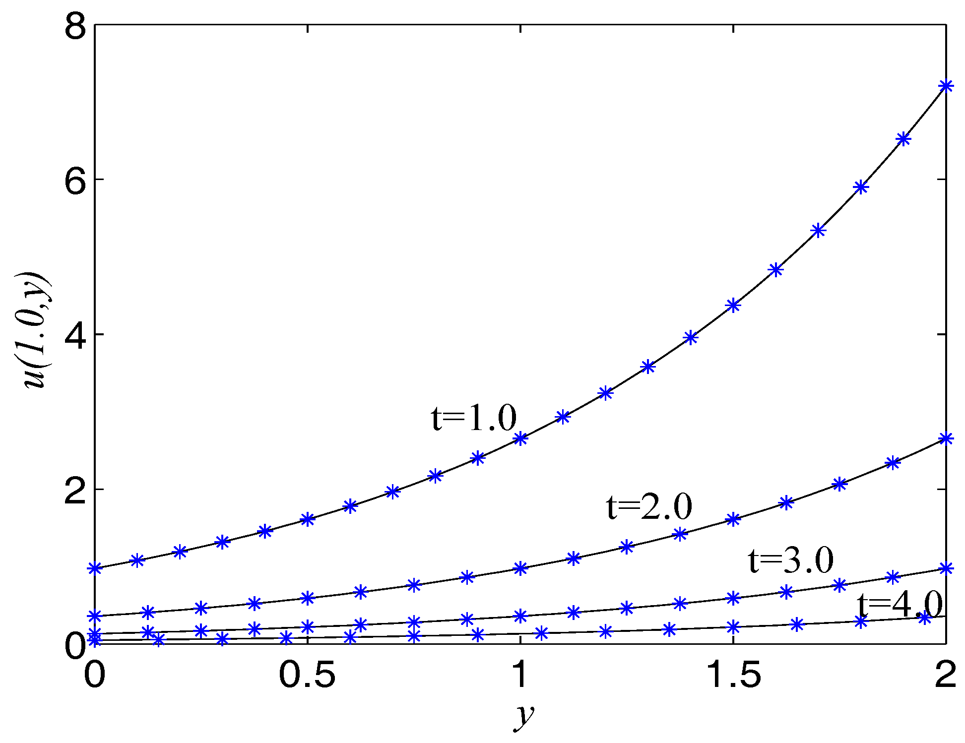
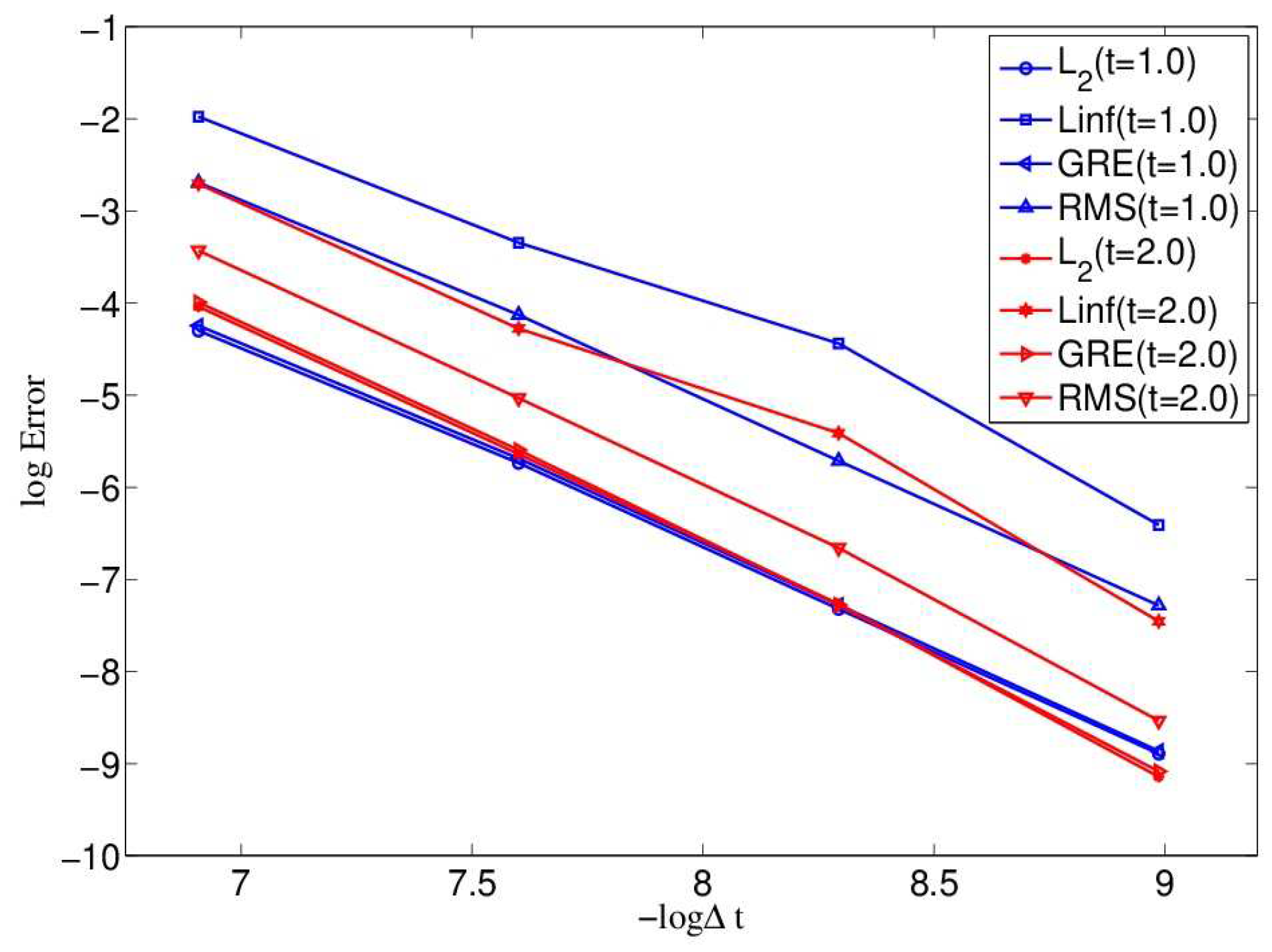
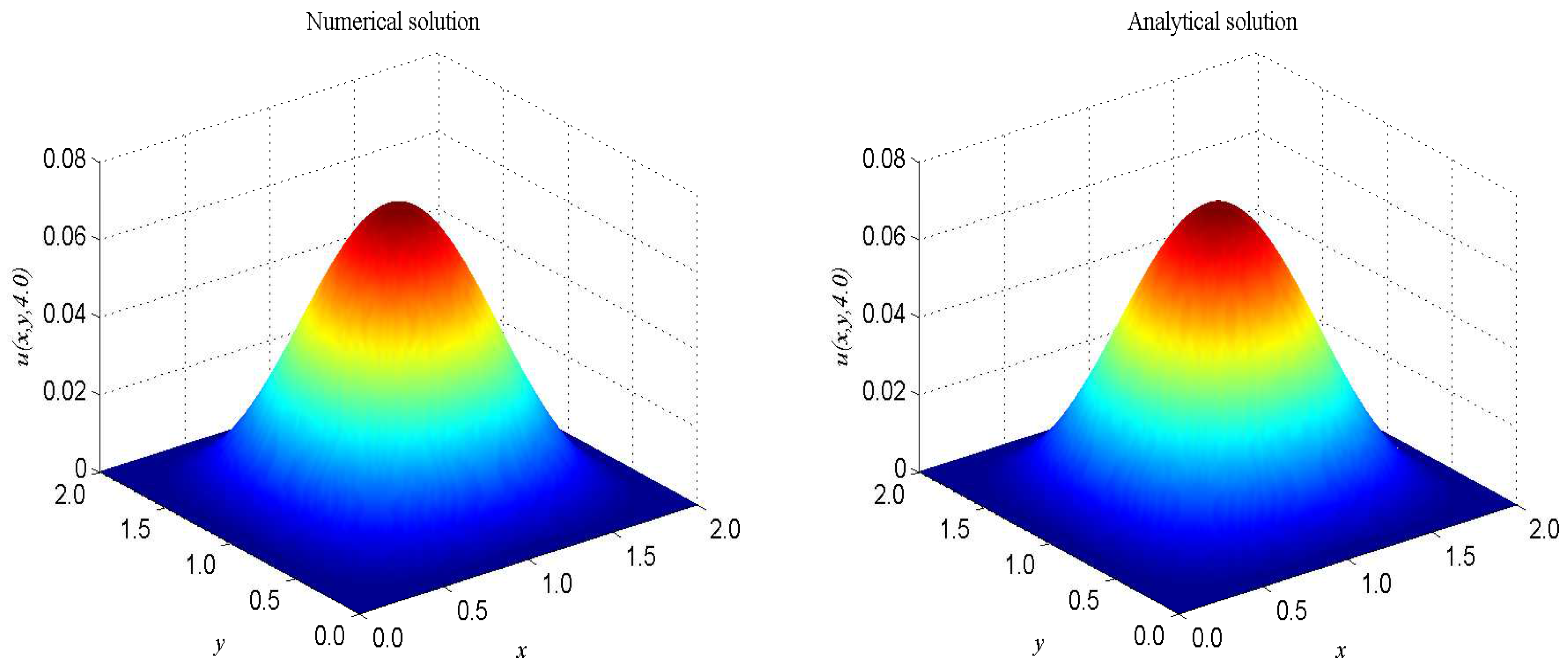
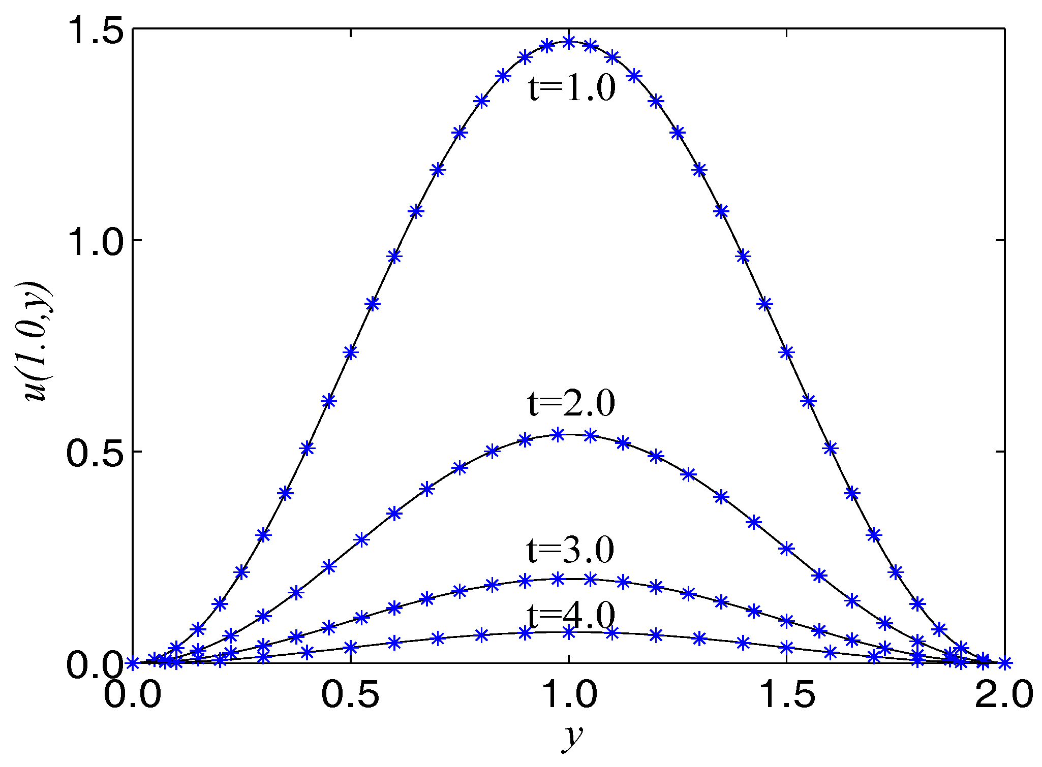
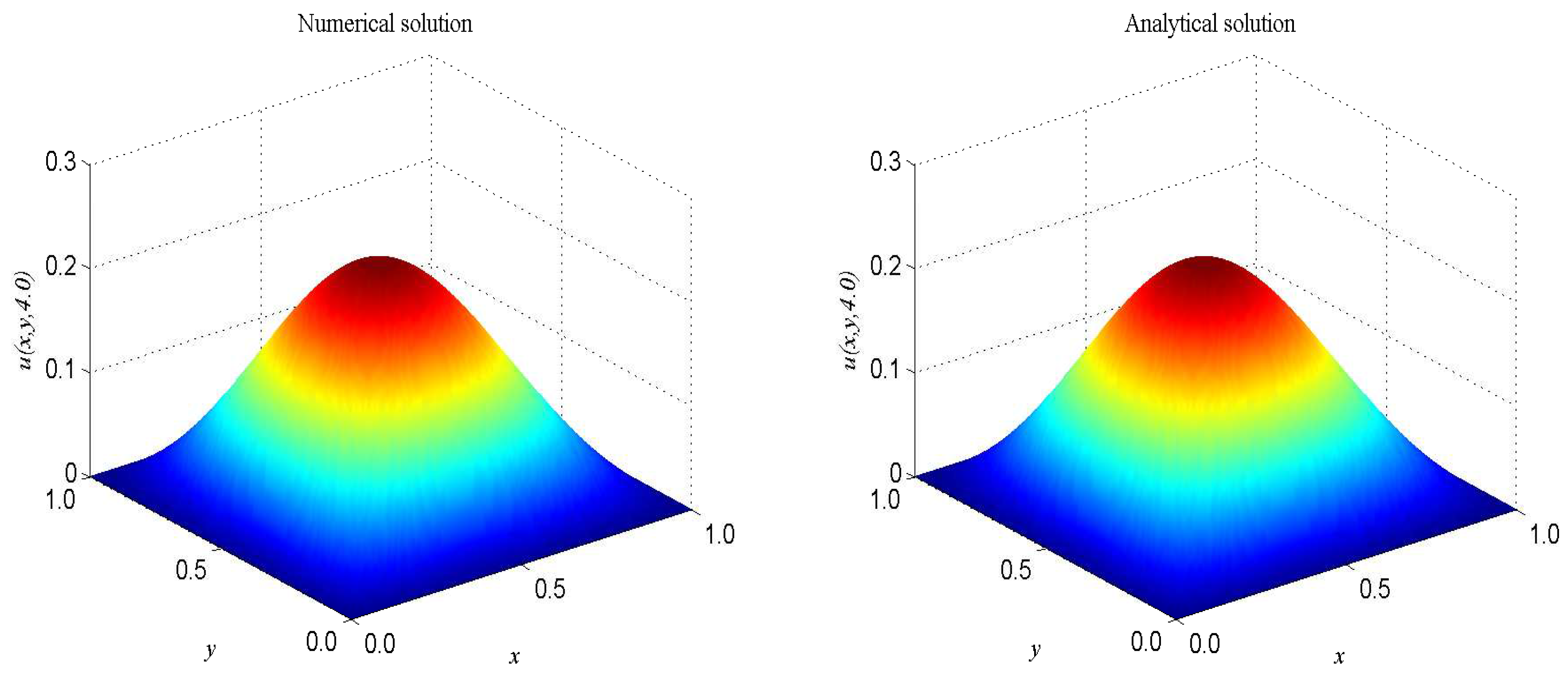
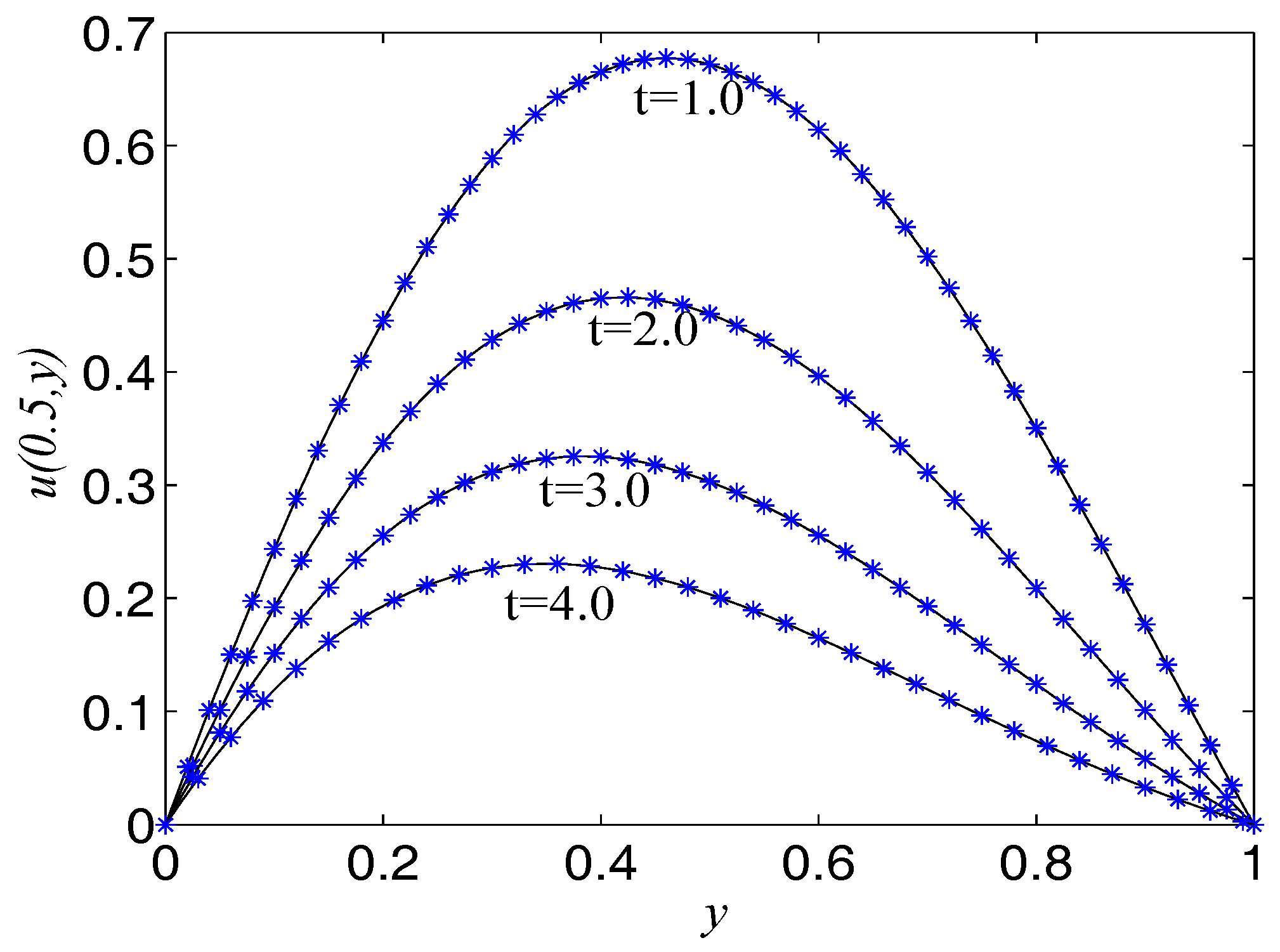
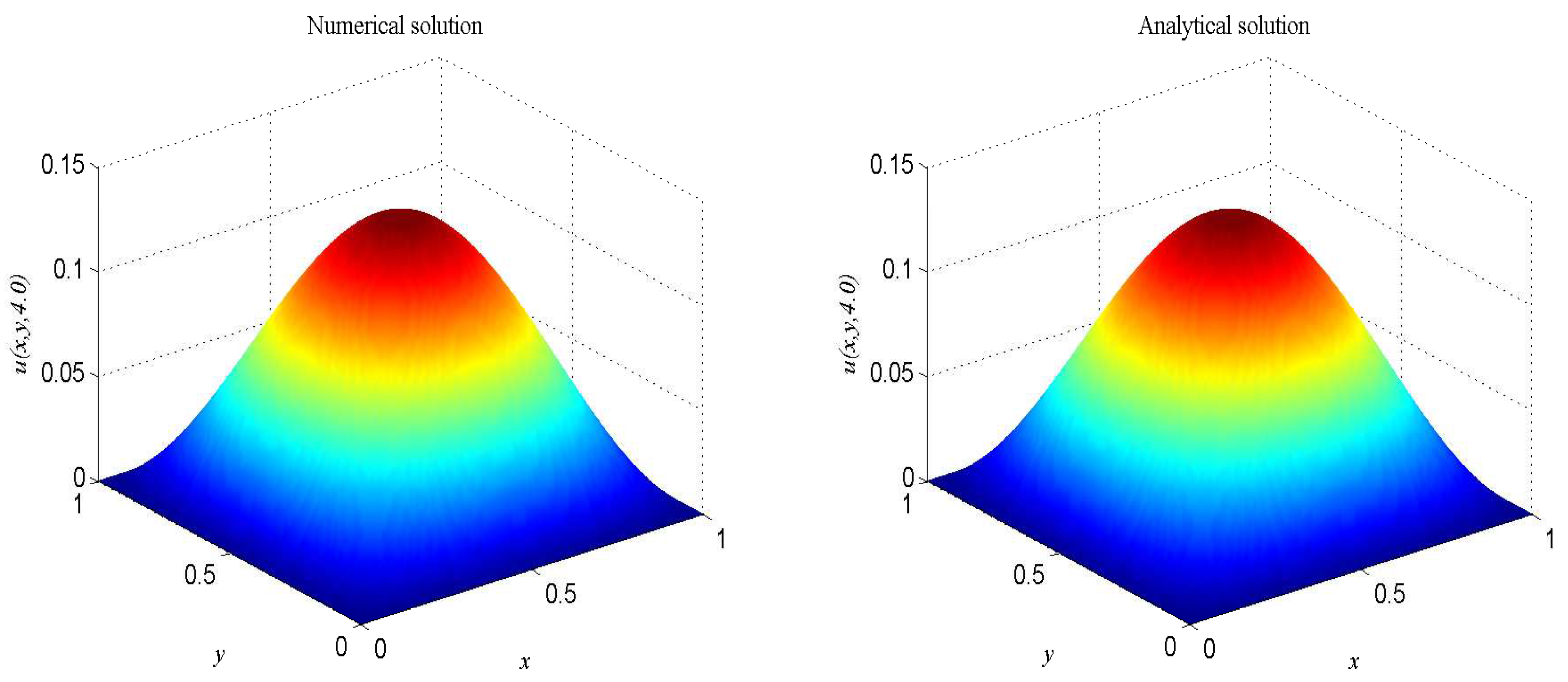
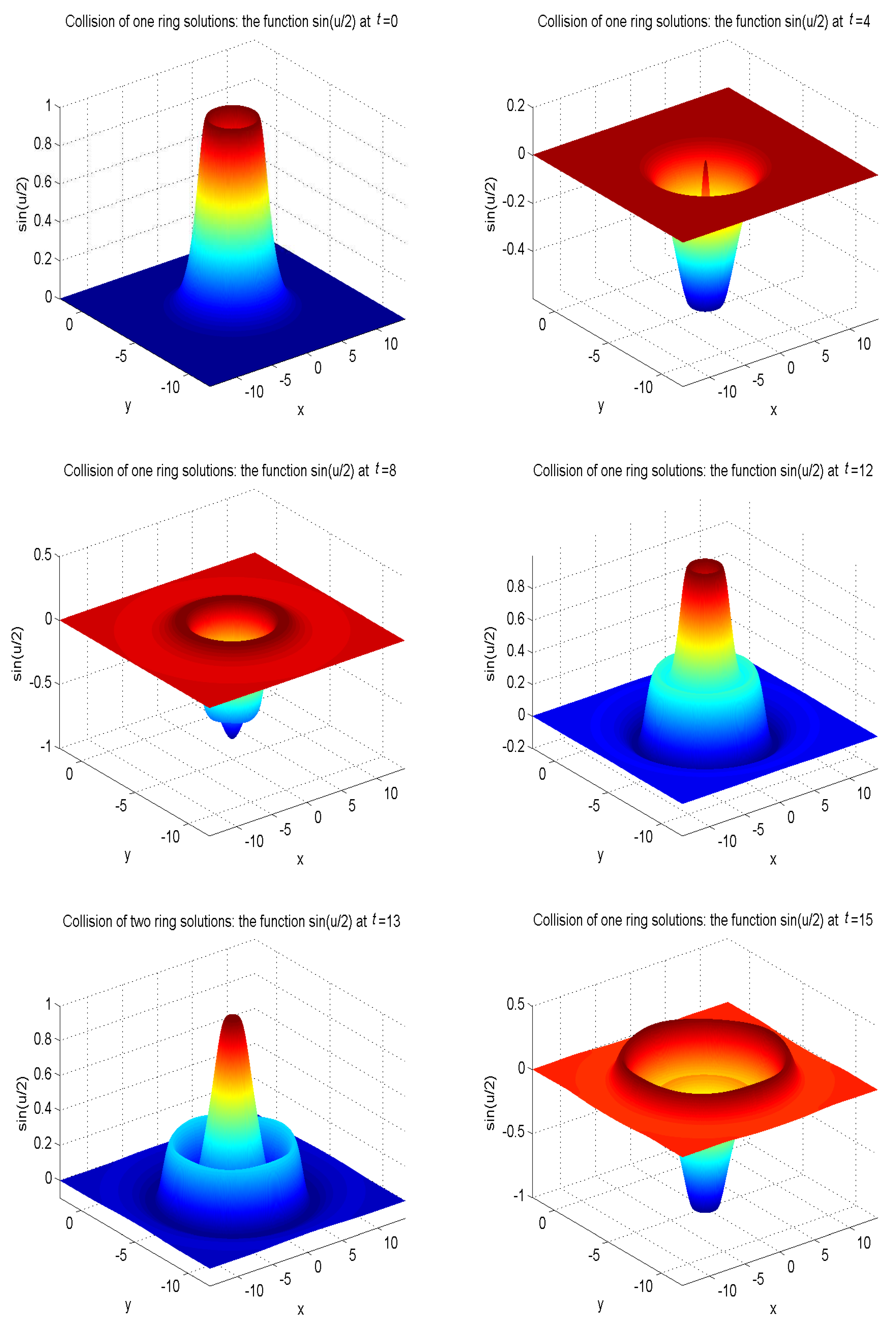
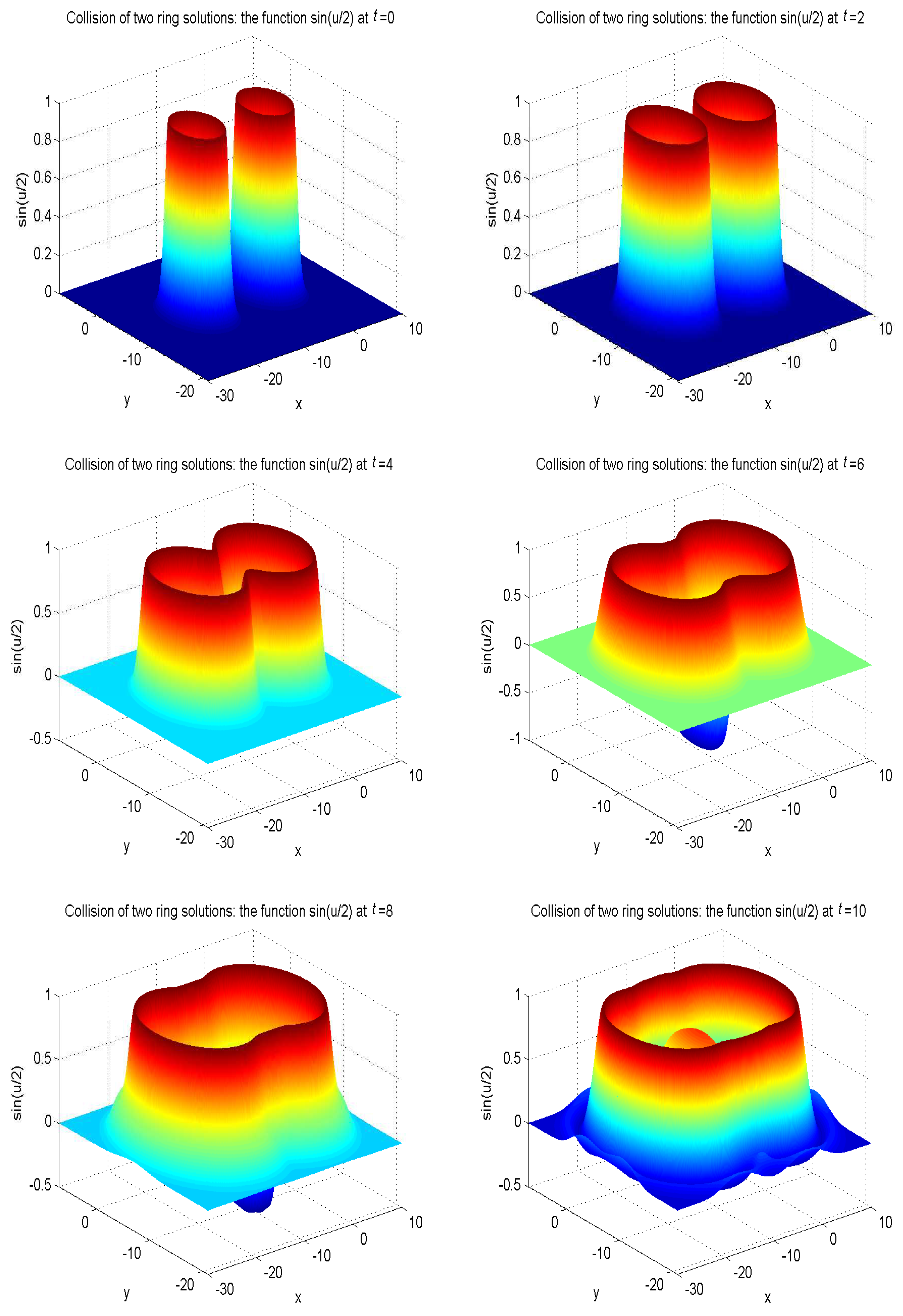
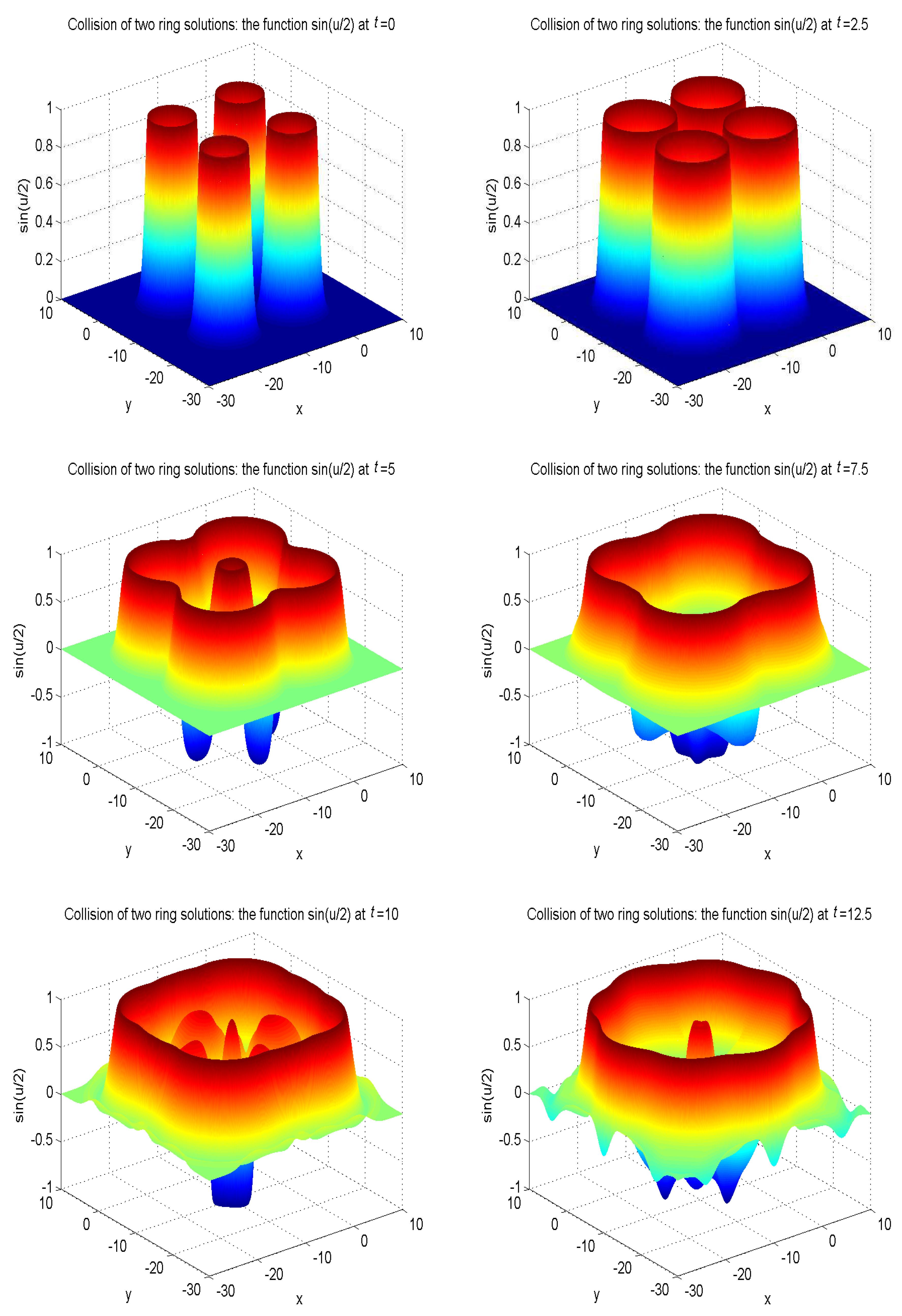
3. Numerical Simulation

In this section, to show the efficiency of the present Lattice BGK model, we give some relevant numerical examples with and without damping terms. In addition, in order to compare with the exact solutions, the efficiency of present model is been tested. We set up the initial condition of distribution function f j ( x , t ) by setting to equal f j e q ( x , t ) for all grid points at t = t 0 . In addition, the macroscopic quantity u ( x , t ) in Equation (1) is also initialized by the given initial condition. The traditional explicit difference scheme t F j ( x , t ) = [ F j ( x , t ) F j ( x , t Δ t ) ] / Δ t can be used for calculating t F j ( x , t ) , here we use the analytic expression. The non-equilibrium extrapolation of distribution function proposed by Guo et al. [57] is applied to handle the boundary conditions. The instructions for the detailed process of boundary treatment are basic and detailed below.
Notice that the distribution function f j can be decomposed into its equilibrium and non-equilibrium parts
f j ( x , t ) = f j ( 0 ) ( x , t ) + f j ( n e q ) ( x , t ) ,
where f j ( 0 ) and f j ( n e q ) are the equilibrium and the non-equilibrium parts of f j .
Through the Chapman-Enskog multiscale analysis for the LBM, we can assume that f j ( n e q ) = ε f j ( 1 ) . For better presentation, we assume x b is a boundary node, and x f is the nearest neighboring grid point of x b at a distance c j Δ t . Thus, the non-equilibrium part of the distribution at grid point x f can be given by
ε f j ( 1 ) ( x f , t ) = f j ( n e q ) ( x f , t ) = f j ( x f , t ) f j ( 0 ) ( x f , t ) .
Notice that the grid point x f is the nearest neighboring grid point x b at a distance Δ x = ε c j , then we have f i ( 1 ) ( x b , t ) = f i ( 1 ) ( x f , t ) + O ( ε ) , and we obtain
f j ( x b , t ) = f j ( 0 ) ( x b , t ) + ε f j ( 1 ) ( x b , t ) = f j ( 0 ) ( x b , t ) + ε [ f i ( 1 ) ( x f , t ) + O ( ε ) ] = f j ( 0 ) ( x b , t ) + ε f i ( 1 ) ( x f , t ) + O ( ε 2 ) = f j ( 0 ) ( x b , t ) + f j ( x f , t ) f j ( 0 ) ( x f , t ) + O ( ε 2 ) ,
where f j ( x f , t ) can be obtained by Equation (4), and f j ( 0 ) ( x b , t ) and f j ( 0 ) ( x f , t ) can be got by Equation (6). Therefore, as long as the macroscopic quantity of the boundary is given, the equilibrium distribution function of the boundary can be obtained, and the distribution function of the boundary can be obtained according to the above non-equilibrium extrapolation Formula (29).
Before simulation and calculation, we need to determine the expression of F j and t F j according to the source term F of the given macroscopic Equation (1), then we can obtain the concrete discrete expression (4).
Next, we will introduce the calculation procedures of the present model as follows:
Step 1: Based on the given conditions u ( x , 0 ) and u t ( x , 0 ) of Equation (2), initialize f j e q ( x , 0 ) by Equation (6).
Step 2: Initialize f j ( x , 0 ) by f j e q ( x , 0 ) from Step 1 in all grid points.
Step 3: Calculate f j ( x , t ) of the inner points by the discrete Boltzmann Equation (4).
Step 4: Calculate u ( x , t ) by Equation (26) and u t ( x , t ) by Equation (5) of the inner points. If the specified termination time is reached, the program stops.
Step 5: Calculate u ( x , t ) and u t ( x , t ) of the boundary points by the given conditions (2).
Step 6: Calculate f j e q ( x , t ) of the boundary points by Equation (6).
Step 7: Calculate f j ( x , t ) of the boundary points by Equation (29).
Step 8: Calculate f j ( x , t + Δ t ) of all grid points by Equation (4), then return to Step 4.
With the present mesoscopic model, we simulate several known exact solutions of the second-order (2 + 1)-dimensional hyperbolic telegraph equation and the (2 + 1)-dimensional damped, driven sine-Gordon equation, respectively. Furthermore, the (2 + 1)-dimensional undamped sine-Gordon equation with different initial condition of various ring solitons are studied to understand the nonlinear behavior characteristics of the system.
Meanwhile, we adopt four different kinds of error norms for measuring the present model’s precision. The root mean square error norm L 2 , max error norm L , global relative error norm GRE and root mean square error norm RMS are generally defined as
(1)
The relative error norm ( L 2 -error)
L 2 = i = 1 N x j = 1 N y | u ( x i , y j , t ) u * ( x i , y j , t ) | 2 1 / 2 / i = 1 N x j = 1 N y | u * ( x i , y j , t ) | 2 1 / 2 .
(2)
The max error norm ( L -error)
L = max i , j | u ( x i , y j , t ) u * ( x i , y j , t ) | .
(3)
The global relative error norm (GRE-error)
GRE = i = 1 N x j = 1 N y | u ( x i , y j , t ) u * ( x i , y j , t ) | / i = 1 N x j = 1 N y | u * ( x i , y j , t ) | .
(4)
The root mean square error norm (RMS-error)
RMS = i = 1 N x j = 1 N y | u ( x i , y j , t ) u * ( x i , y j , t ) | 2 / ( N x × N y ) 1 / 2 .
Here, u ( x i , y j , t ) , u * ( x i , y j , t ) are numerical solution and exact solution, respectively. The summation is added up from the information of all mesh points. Results show that the numerical solutions agree fairly well with the exact solutions over a considerable period of time.
Example 1.
Consider the following (2 + 1)-dimensional hyperbolic telegraph equation in the region 0 x 2 , 0 y 2 as follows:
2 u t 2 + 2 u t + u = 2 u x 2 + 2 u y 2 2 e x + y t ,
the initial conditions are given below
u ( x , y , 0 ) = e x + y , u t ( x , y , 0 ) = e x + y .
The exact solution for the current problem is given in Ref. [5] by
u ( x , y , t ) = e x + y t .
The boundary conditions are given from the exact solution.
In numerical simulation, we take F ( x , t ) = u 2 u / t 2 e x + y t , α = 2 , β = 1 , Δ x = Δ y = 0.025 , c = 200 . The computational domain is pinned to Ω = [ 0 , 2 ] × [ 0 , 2 ] . We present the surface graph of the numerical and exact solutions by the present lattice BGK model at t = 4.0 , see Figure 1. For clarity of contrast, we also demonstrate the two-dimensional contrast diagrams at x = 1.0 for specific different times: t = 1.0 , t = 2.0 , t = 3.0 and t = 4.0 , see Figure 2. The relative error norm L 2 , the max error norm L , the global relative error GRE norm and the root mean square error RMS norm for the solutions of the second-order hyperbolic telegraph equation at different instants of time can be found in Table 1.
To measure the accuracy of the present mesoscopic model, the relative error, max error, global relative error and root mean square error are shown in Figure 3 at different time t = 1.0 and t = 2.0 with different resolutions, range from Δ t = 1.25 × 10 4 to Δ t = 10 3 and c = 25 to 200, with N x = N y = 80 . It is found that the present mesoscopic model is of second-order time accuracy. The order of the maximum error norm increases from 2.0720 to 2.2868, the order of the global relative error norm increases from 2.0789 to 2.2968, and the order of the root mean square error norm increases from 2.0720 to 2.2865.
Example 2.
Consider the following (2 + 1)-dimensional hyperbolic equation in the area 0 x 2 , 0 y 2 given by
2 u t 2 + u t = 2 u x 2 + 2 u y 2 2 sin u + 2 sin [ e t ( 1 cos ( π x ) ) ( 1 cos ( π y ) ) ] π 2 e t [ cos ( π x ) + cos ( π y ) 2 cos ( π x ) cos ( π y ) ] ,
the initial conditions are given below
u ( x , y , 0 ) = ( 1 cos ( π x ) ) ( 1 cos ( π y ) ) , u t ( x , y , 0 ) = ( 1 cos ( π x ) ) ( 1 cos ( π y ) ) .
The exact solution for this instance is given in Ref. [6] by
u ( x , y , t ) = e t ( 1 cos ( π x ) ) ( 1 cos ( π y ) ) .
The boundary conditions are given from the exact solution from Equation (39).
The term ’ sin u ’ is a very good representation of nonlinearity. In the proceeding, we take F ( x , t ) = 2 sin u + 2 sin [ e t ( 1 cos ( π x ) ) ( 1 cos ( π y ) ) ] π 2 e t [ cos ( π x ) + cos ( π y ) 2 cos ( π x ) cos ( π y ) ] , α = β = 1 , Δ x = Δ y = 0.025 , c = 200 . The computational domain is pinned to Ω = [ 0 , 2 ] × [ 0 , 2 ] . We present the spatio-temporal evolution of the numerical and exact solutions by the present model at t = 4.0 , see Figure 4. For clarity of contrast, we also present the two-dimensional contrast diagrams at x = 1.0 for especial different times: t = 1.0 , t = 2.0 , t = 3.0 and t = 4.0 , see Figure 5. The maximum value of the wave decays slowly over time due to the damping term and the source term. The relative error L 2 , max error norm L , global relative error norm GRE and root mean square error norm RMS for the solutions of the second-order hyperbolic telegraph equation at specific times can be found in Table 2.
Example 3.
Consider the following (2 + 1)-dimensional hyperbolic equation in the area 0 x 1 , 0 y 1 given by
2 u t 2 + 4 π u t + 2 π 2 u = 2 u x 2 + 2 u y 2 + 2 π t sin [ π ( x + y ) ] e ( x + y ) t + [ ( x + y 2 π ) 2 2 t 2 ] sin ( π x ) sin ( π y ) e ( x + y ) t ,
the initial conditions are given below
u ( x , y , 0 ) = sin ( π x ) sin ( π y ) , u t ( x , y , 0 ) = sin ( π x ) sin ( π y ) .
The exact solution for this instance is given in Ref. [7] by
u ( x , y , t ) = e ( x + y ) t sin ( π x ) sin ( π y ) .
The boundary conditions are given from the exact solution.
In the proceeding, we take F ( x , t ) = u 2 ( 1 + π 2 ) u / t , α = 2 ( 1 + π 2 ) , β = 1 , Δ x = Δ y = 0.0125 , c = 500 . The computational domain is pinned to Ω = [ 0 , 1 ] × [ 0 , 1 ] . We present the spatio-temporal evolution of the numerical and exact solutions by the LBM at t = 4.0 , see Figure 6. For clarity of contrast, we also present the two-dimensional contrast diagrams at x = 0.5 for some specific times: t = 1.0 , t = 2.0 , t = 3.0 and t = 4.0 , see Figure 7. The relative error norm L 2 , max error norm L , global relative error norm GRE and root mean square error norm RMS for the solutions of the second-order hyperbolic telegraph equation at specific times can be found in Table 3.
Example 4.
Consider the following (2 + 1)-dimensional hyperbolic equation in the area 0 x 1 , 0 y 1 given by
2 u t 2 + 1 2 u t + 4 u = 2 u x 2 + 2 u y 2 + 2 ( π 2 + 2 ) e 0 . 5 t sin ( π x ) sin ( π y ) ,
the initial conditions are given below
u ( x , y , 0 ) = sin ( π x ) sin ( π y ) , u t ( x , y , 0 ) = 0 . 5 sin ( π x ) sin ( π y ) .
The exact solution for this instance is given in Ref. [7] by
u ( x , y , t ) = e 0.5 t sin ( π x ) sin ( π y ) .
The boundary conditions are given from the exact solution.
In the proceeding, we take F ( x , t ) = 4 u 0.5 u / t + 2 ( π 2 + 2 ) e 0.5 t sin ( π x ) sin ( π y ) , α = 0.5 , β = 1 , Δ x = Δ y = 0.0125 , c = 500 . The computational domain is pinned to Ω = [ 0 , 1 ] × [ 0 , 1 ] . We present the spatio-temporal evolution of the numerical and exact solutions by the present model at t = 4.0 , see Figure 8. For clarity of contrast, we also present the two-dimensional contrast diagrams at x = 0.5 for specific different times: t = 1.0 , t = 2.0 , t = 3.0 and t = 4.0 , see Figure 9. The relative error norm L 2 , max error norm L , global relative error norm GRE and root mean square error norm RMS for the solutions of the second-order hyperbolic telegraph equation at specific times can be found in Table 4.
Example 5.
Consider the following (2 + 1)-dimensional sine-Gordon equation [58] given by
2 u t 2 = 2 u x 2 + 2 u y 2 sin u ,
in the area a < x < a , b < y < b .
We simulate some particular cases of specific initial conditions with various numbers of circular ring solutions to study the nonlinear behaviors of the system. Numerical examples are carried out for three cases:
The first initial condition of one ring solitons is as follows:
u ( x , y , 0 ) = α arctan exp ( 3 x 2 + y 2 ) , u t ( x , y , 0 ) = 0 ,
where 14 x , y 14 .
The second initial condition of two ring solitons is the following:
u ( x , y , 0 ) = α j = 1 2 arctan exp γ 4 ( x + x j ) 2 + ( y + y j ) 2 , u t ( x , y , 0 ) = β j = 1 2 sech γ 4 ( x + x j ) 2 + ( y + y j ) 2 ,
where 30 x 10 , 21 y 7 , { ( x j , y j ) } = { ( 3 , 7 ) , ( 17 , 7 ) } .
The third initial condition of four ring solitons is as follows:
u ( x , y , 0 ) = α j = 1 4 arctan exp γ 4 ( x + x j ) 2 + ( y + y j ) 2 , u t ( x , y , 0 ) = β j = 1 4 sech γ 4 ( x + x j ) 2 + ( y + y j ) 2 ,
where 30 x 10 , 30 y 10 , { ( x j , y j ) } = { ( 3 , 3 ) , ( 3 , 17 ) , ( 17 , 3 ) , ( 17 , 17 ) } .
In our simulations, the zero gradient is used to deal with the boundary of the domain as u ( x b , t ) = u ( x f , t ) , where x b is a boundary node, and x f is the nearest neighboring grid point of x b at a distance c j Δ t . The model parameters are set as α = 4 , β = 4.13 , γ = 1 / 0.436 . The other parameters are given as α = 1 , β = 0 , Δ x = Δ y = 0.05 , c = 50 . To better display the nonlinear propagation process of the wave, we present the surface graph of numerical solutions of collision of one ring solitons in regard to sin ( u / 2 ) at t = 0 , t = 4.0 , t = 8.0 , t = 12.0 , t = 13.0 , t = 15.0 , see Figure 10. The surface graph of numerical solutions of collision of two ring solitons in regard to sin ( u / 2 ) at t = 0 , t = 4.0 , t = 8.0 , t = 12.0 , t = 13.0 , t = 15.0 , see Figure 11. The surface graph of numerical solutions of collision of four ring solitons in regard to sin ( u / 2 ) at t = 0 , t = 2.5 , t = 5.0 , t = 7.5 , t = 10.0 , t = 12.5 , see Figure 12.
It can be found that the solitons reveal potent nonlinear evolution characteristics as time passed. One of the distinct features of solitons is that they can evolve without phanic changes in their identity after interplay. These numerical simulation results are in accordance with those results in Ref. [58].

4. Conclusions

Based on the mesoscopic lattice BGK method, we have investigated the numerical solution of (2 + 1)-dimensional wave equation with nonlinear damping and source terms, such as the hyperbolic telegraph equation, damped or undamped sine-Gordon equation, and so on. With the help of the Chapman-Enskog multiscale expansion, the macroscopic dynamical evolution equation can be precisely obtained from the present mesoscopic scheme in the continuity system without appending any amending term. Through observation, we can find that for the sine-Gordon system without damping terms and other source terms, the crest of the wave will oscillate up and down, and at the same time, the waveform will deform in the form of two or four crests that have evolved into one over time. All these phenomena reflect the evolution characteristics of nonlinear systems. Numerical examples for some test issues have been held to check the present mesoscopic model. The numerical solutions are in well coincident with the exact ones. From the convergence research of the Example 1, it can be found that the present mesoscopic model has the second-order accuracy in time. It is believed that with this model, we can predict and enrich the characterization and description of the nonlinear behavior characteristics in complex nonlinear dynamic systems.

Author Contributions

Conceptualization, D.L., H.L. and B.S.; Methodology, B.S. and H.L.; Investigation, D.L.; Validation, D.L. and H.L.; Visualization, D.L.; Writing-original draft preparation, D.L.; Writing-review and editing, B.S. and H.L.; Supervision, H.L.; Project administration, H.L.; Funding acquisition, H.L.

Funding

This research was supported by National Natural Science Foundation of China (under Grant No. 11301082) and Natural Science Foundation of Fujian Provinces (under Grant Nos. JT180075, 2018J01654).

Acknowledgments

We sincerely appreciate the referees’ valuable suggestions to improve our work.

Conflicts of Interest

The authors declare no conflict of interest.

References

  1. Abdou, M.A.; Soliman, A.A. Variational iteration method for solving Burger’s and coupled Burger’s equations. J. Comput. Appl. Math. 2005, 181, 245–251. [Google Scholar] [CrossRef]
  2. Ӧzpınar, F. Applying discrete homotopy analysis method for solving fractional partial differential equations. Entropy 2018, 20, 332. [Google Scholar]
  3. Petrila, T.; Trif, D. Introduction to Numberical Solutions for Ordinary and Partial Differential Equations. In Basics of Fluid Mechanics and Introduction to Computational Fluid Dynamics; Springer: Boston, MA, USA, 2005; pp. 197–246. [Google Scholar]
  4. Chang, C.W.; Liu, C.S. An implicit Lie-group iterative scheme for solving the nonlinear Klein-Gordon and sine-Gordon equations. Appl. Math. Model. 2016, 40, 1157–1167. [Google Scholar] [CrossRef]
  5. Dehghan, M.; Shokri, A. A meshless method for numerical solution of a linear hyperbolic equation with variable coefficients in two space dimensions. Numer. Methods Part. Differ. Equ. 2009, 25, 494–506. [Google Scholar] [CrossRef]
  6. Liu, W.J.; Sun, J.B.; Wu, B.Y. Space-time spectral method for the two-dimensional generalized sine-Gordon equation. J. Math. Anal. Appl. 2015, 427, 787–804. [Google Scholar] [CrossRef]
  7. Ding, H.F.; Zhang, Y.X. A new fourth-order compact finite difference scheme for the two-dimensional second-order hyperbolic equation. J. Comput. Appl. Math. 2009, 230, 626–632. [Google Scholar] [CrossRef] [Green Version]
  8. Shi, D.Y.; Pei, L.F. Nonconforming quadrilateral finite element method for a class of nonlinear sine-Gordon equations. Appl. Math. Comput. 2013, 219, 9447–9460. [Google Scholar] [CrossRef]
  9. Benzi, R.; Succi, S.; Vergasola, M. The lattice Boltzmann equation: Theory and applications. Phys. Rep. 1992, 222, 145–197. [Google Scholar] [CrossRef]
  10. Chen, S.Y.; Doolen, G.D. Lattice Boltzmann method for fluid flows. Annu. Rev. Fluid Mech. 1998, 30, 329–364. [Google Scholar] [CrossRef]
  11. Xu, A.G.; Zhang, G.C.; Ying, Y.J.; Wang, C. Complex fields in heterogeneous materials under shock: Modeling, simulation and analysis. Sci. China Phys. Mech. Astron. 2016, 59, 650501. [Google Scholar] [CrossRef]
  12. Li, Q.; Luo, K.H.; Kang, Q.J.; He, Y.L.; Chen, Q.; Liu, Q. Lattice Boltzmann methods for multiphase flow and phase-change heat transfer. Prog. Energy Combust. Sci. 2016, 52, 62–105. [Google Scholar] [CrossRef] [Green Version]
  13. Christensen, A.; Graham, S. Multiscale lattice Boltzmann modeling of phonon transport in crystalline semiconductor materials. Numer. Heat Transf. B 2010, 57, 89–109. [Google Scholar] [CrossRef]
  14. Li, Q.; Luo, K.H.; Gao, Y.J.; He, Y.L. Additional interfacial force in lattice Boltzmann models for incompressible multiphase flows. Phys. Rev. E 2012, 85, 026704. [Google Scholar] [CrossRef] [PubMed]
  15. Wang, Y.; Shu, C.; Teo, C.J. Thermal lattice Boltzmann flux solver and its application for simulation of incompressible thermal flows. Comput. Fluids 2014, 94, 98–111. [Google Scholar] [CrossRef]
  16. Wang, Y.; Shu, C.; Huang, H.B.; Teo, C.J. Multiphase lattice Boltzmann flux solver for incompressible multiphase flows with large density ratio. J. Comput. Phys. 2015, 280, 404–423. [Google Scholar] [CrossRef]
  17. Wang, Y.; Yang, L.M.; Shu, C. From lattice Boltzmann method to lattice Boltzmann flux solver. Entropy 2015, 17, 7713–7735. [Google Scholar] [CrossRef]
  18. Wei, Y.K.; Wang, Z.D.; Qian, Y.H. A numerical study on entropy generation in two-dimensional Rayleigh-Bénard convection at different Prandtl number. Entropy 2017, 19, 443. [Google Scholar] [CrossRef]
  19. Wei, Y.K.; Wang, Z.D.; Qian, Y.H.; Guo, W.J. Study on bifurcation and dual solutions in natural convection in a horizontal annulus with rotating inner cylinder using thermal immersed boundary-lattice Boltzmann method. Entropy 2018, 20, 733. [Google Scholar] [CrossRef]
  20. Yang, X.Y.; He, H.Z.; Xu, J.; Wei, Y.K.; Zhang, H. Entropy generation rates in two-dimensional Rayleigh-Taylor turbulence mixing. Entropy 2018, 20, 738. [Google Scholar] [CrossRef]
  21. Wei, Y.K.; Dou, H.S.; Qian, Y.H.; Wang, Z.D. A novel two-dimensional coupled lattice Boltzmann model for incompressible flow in application of turbulence Rayleigh-Taylor instability. Comput. Fluids 2017, 156, 97–102. [Google Scholar] [CrossRef]
  22. Wei, Y.K.; Yang, H.; Dou, H.S.; Lin, Z.; Wang, Z.D.; Qian, Y.H. A novel two-dimensional coupled lattice Boltzmann model for thermal incompressible flows. Appl. Math. Comput. 2018, 339, 556–567. [Google Scholar] [CrossRef]
  23. Yuan, H.Z.; Niu, X.D.; Shu, S.; Li, M.J.; Yamaguchi, H. A momentum exchange-based immersed boundary-lattice Boltzmann method for simulating a flexible filament in an incompressible flow. Comput. Math. Appl. 2014, 67, 1039–1056. [Google Scholar] [CrossRef]
  24. Yuan, H.Z.; Wang, Y.; Shu, C. An adaptive mesh refinement-multiphase lattice Boltzmann flux solver for simulation of complex binary fluid flows. Phys. Fluids 2017, 29, 123604. [Google Scholar] [CrossRef]
  25. Yuan, H.Z.; Chen, Z.; Shu, C.; Wang, Y.; Niu, X.D.; Shu, S. A free energy-based surface tension force model for simulation of multiphase flows by level-set method. J. Comput. Phys. 2017, 345, 404–426. [Google Scholar] [CrossRef]
  26. Xu, A.G.; Lin, C.D.; Zhang, G.C.; Li, Y.J. Multiple-relaxation-time lattice Boltzmann kinetic model for combustion. Phys. Rev. E 2015, 91, 043306. [Google Scholar] [CrossRef] [PubMed]
  27. Gan, Y.B.; Xu, A.G.; Zhang, G.C.; Succi, S. Discrete Boltzmann modeling of multiphase flows: Hydrodynamic and thermodynamic non-equilibrium effects. Soft Matter 2015, 11, 5336–5345. [Google Scholar] [CrossRef] [PubMed]
  28. Gan, Y.B.; Xu, A.G.; Zhang, G.C.; Zhang, Y.D.; Succi, S. Discrete Boltzmann trans-scale modeling of high-speed compressible flows. Phys. Rev. E 2018, 97, 053312. [Google Scholar] [CrossRef] [PubMed] [Green Version]
  29. Zhang, Y.D.; Xu, A.G.; Zhang, G.C.; Zhu, C.M.; Lin, C.D. Kinetic modeling of detonation and effects of negative temperature coefficient. Combust Flame 2016, 173, 483–492. [Google Scholar] [CrossRef]
  30. Zhang, Y.D.; Xu, A.G.; Zhang, G.C.; Chen, Z.H.; Wang, P. Discrete ellipsoidal statistical BGK model and Burnett equations. Front. Phys. 2018, 13, 135101. [Google Scholar] [CrossRef] [Green Version]
  31. Zhang, Y.D.; Xu, A.G.; Zhang, G.C.; Gan, Y.B.; Chen, Z.H.; Succi, S. Entropy production in thermal phase separation: A kinetic-theory approach. Soft Matter 2019, 15, 2245–2259. [Google Scholar] [CrossRef]
  32. Xu, A.G.; Zhang, G.C.; Zhang, Y.D.; Wang, P.; Ying, Y.J. Discrete Boltzmann model for implosion- and explosion-related compressible flow with spherical symmetry. Front. Phys. 2018, 13, 135102. [Google Scholar] [CrossRef]
  33. Gan, Y.B.; Xu, A.G.; Zhang, G.C.; Lin, C.D.; Lai, H.L.; Liu, Z.P. Nonequilibrium and morphological characterizations of Kelvin-Helmholtz instability in compressible flows. Front. Phys. 2019, 14, 43602. [Google Scholar] [CrossRef]
  34. Lin, C.D.; Xu, A.G.; Zhang, G.C.; Li, Y.J. Double-distribution-function discrete Boltzmann model for combustion. Combust Flame 2016, 164, 137–151. [Google Scholar] [CrossRef] [Green Version]
  35. Lin, C.D.; Xu, A.G.; Zhang, G.C.; Luo, K.H.; Li, Y.J. Discrete Boltzmann modeling of Rayleigh-Taylor instability in two-component compressible flows. Phys. Rev. E 2017, 96, 053305. [Google Scholar] [CrossRef] [PubMed]
  36. Lin, C.D.; Luo, K.H. MRT discrete Boltzmann method for compressible exothermic reactive flows. Combust Flame 2018, 166, 176–183. [Google Scholar] [CrossRef]
  37. Lai, H.L.; Xu, A.G.; Zhang, G.C.; Gan, Y.B.; Ying, Y.J.; Succi, S. Nonequilibrium thermohydrodynamic effects on the Rayleigh-Taylor instability in compressible flows. Phys. Rev. E 2016, 94, 023106. [Google Scholar] [CrossRef] [PubMed]
  38. Zhang, Q.Y.; Sun, D.K.; Zhang, Y.F.; Zhu, M.F. Numerical modeling of condensate droplet on superhydrophobic nanoarrays using the lattice Boltzmann method. Chin. Phys. B 2016, 25, 066401. [Google Scholar] [CrossRef]
  39. Sun, D.K.; Chai, Z.H.; Li, Q.; Lin, G. A lattice Boltzmann-cellular automaton study on dendrite growth with melt convection in solidification of ternary alloys. Chin. Phys. B 2018, 27, 088105. [Google Scholar] [CrossRef]
  40. Li, Q.; Kang, Q.J.; Francois, M.M.; He, Y.L.; Luo, K.H. Lattice Boltzmann modeling of boiling heat transfer: The boiling curve and the effects of wettability. Int. J. Heat Mass Transf. 2015, 85, 787–796. [Google Scholar] [CrossRef] [Green Version]
  41. Gao, Y.; Le, L.H.; Shi, B.C. Numerical solution of Burgers’ equation by lattice Boltzmann method. Appl. Math. Comput. 2013, 219, 7685–7692. [Google Scholar] [CrossRef]
  42. Lai, H.L.; Ma, C.F. A new lattice Boltzmann model for solving the coupled viscous Burgers’ equation. Physica A 2014, 395, 445–457. [Google Scholar] [CrossRef]
  43. Wang, H.M. Solitary wave of the Korteweg-de Vries equation based on lattice Boltzmann model with three conservation laws. Adv. Space Res. 2017, 59, 283–292. [Google Scholar] [CrossRef]
  44. Wang, H.M.; Yan, G.W. Lattice Boltzmann model for the interaction of (2 + 1)-dimensional solitons in generalized Gross-Pitaevskii equation. Appl. Math. Model. 2016, 40, 5139–5152. [Google Scholar] [CrossRef]
  45. Shi, B.C.; Guo, Z.L. Lattice Boltzmann model for nonlinear convection-diffusion equations. Phys. Rev. E 2009, 79, 016701. [Google Scholar] [CrossRef]
  46. Chai, Z.H.; He, N.Z.; Guo, Z.L.; Shi, B.C. Lattice Boltzmann model for high-order nonlinear partial differential equations. Phys. Rev. E 2018, 97, 013304. [Google Scholar] [CrossRef] [PubMed] [Green Version]
  47. Chai, Z.H.; Zhao, T.S. Lattice Boltzmann model for the convection-diffusion equation. Phys. Rev. E 2013, 87, 063309. [Google Scholar] [CrossRef] [Green Version]
  48. Yoshida, H.; Nagaoka, M. Lattice Boltzmann method for the convection-diffusion equation in curvilinear coordinate systems. J. Comput. Phys. 2014, 257, 884–900. [Google Scholar] [CrossRef]
  49. Wang, L.; Shi, B.C.; Chai, Z.H. Regularized lattice Boltzmann model for a class of convection-diffusion equations. Phys. Rev. E 2015, 92, 043311. [Google Scholar] [CrossRef] [PubMed]
  50. Wang, L.; Chai, Z.H.; Shi, B.C. Regularized lattice Boltzmann simulation of double-diffusive convection of power-law nanofluids in rectangular enclosures. Int. J. Heat Mass Transf. 2016, 102, 381–395. [Google Scholar] [CrossRef]
  51. Chai, Z.H.; Shi, B.C.; Guo, Z.L. A multiple-relaxation-time lattice Boltzmann model for general nonlinear anisotropic convection-diffusion equations. J. Sci. Comput. 2016, 69, 355–390. [Google Scholar] [CrossRef]
  52. Lai, H.L.; Ma, C.F. Lattice Boltzmann method for the generalized Kuramoto-Sivashinsky equation. Physica A 2009, 388, 1405–1412. [Google Scholar] [CrossRef]
  53. Yan, G.W. A lattice Boltzmann equation for waves. J. Comput. Phys. 2000, 161, 61–69. [Google Scholar]
  54. Lai, H.L.; Ma, C.F. Lattice Boltzmann model for generalized nonlinear wave equations. Phys. Rev. E 2011, 84, 046708. [Google Scholar] [CrossRef]
  55. Shi, B.C.; Guo, Z.L. Lattice Boltzmann model for the one-dimensional nonlinear Dirac equation. Phys. Rev. E 2009, 79, 066704. [Google Scholar] [CrossRef]
  56. Chai, Z.H.; Shi, B.C. A novel lattice Boltzmann model for the Poisson equation. Appl. Math. Model. 2008, 32, 2050–2058. [Google Scholar] [CrossRef]
  57. Guo, Z.L.; Zheng, C.G.; Shi, B.C. An extrapolation method for boundary conditions in lattice Boltzmann method. Phys. Fluids 2002, 14, 2007–2010. [Google Scholar] [CrossRef]
  58. Sheng, Q.; Khaliq, A.Q.M.; Voss, D.A. Numerical simulation of two-dimensional sine-Gordon solitons via a split cosine scheme. Math. Comput. Simul. 2005, 68, 355–373. [Google Scholar] [CrossRef]
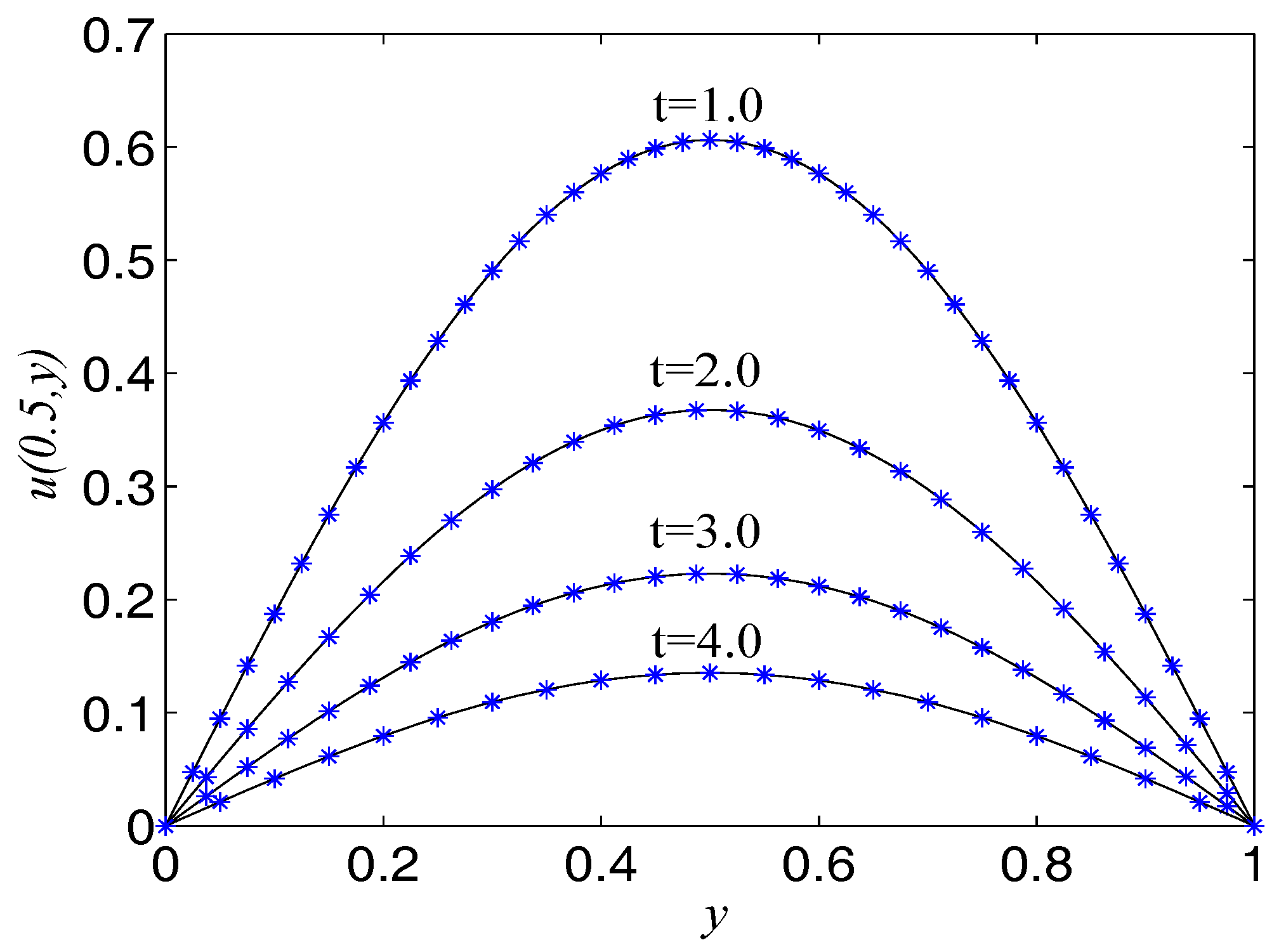
Figure 1. Spatio-temporal evolution of the numerical (left) and exact (right) solutions at t = 4.0 for Example 1.
Entropy 21 00390 g001
Figure 2. Comparison of numerical solutions with exact ones at x = 1.0 at different times for Example 1. The solid lines are drawn as the exact solutions.
Entropy 21 00390 g002
Figure 3. Accuracy test at t = 1.0 and 2.0 with N x = N y = 80 for Example 1.
Entropy 21 00390 g003
Figure 4. Spatio-temporal evolution of the numerical (left) and exact (right) solutions at t = 4.0 for Example 2.
Entropy 21 00390 g004
Figure 5. Comparison of numerical solutions with exact ones at x = 1.0 at different instants of time for Example 2. The solid lines are drawn as the exact solutions.
Entropy 21 00390 g005
Figure 6. Spatio-temporal evolution of the numerical (left) and exact (right) solutions at t = 4.0 for Example 3.
Entropy 21 00390 g006
Figure 7. Comparison of numerical solutions with exact ones at x = 0.5 at specific times for Example 3. The solid lines are drawn as the exact solutions.
Entropy 21 00390 g007
Figure 8. Spatio-temporal evolution of the numerical (left) and exact (right) solutions at t = 4.0 for Example 4.
Entropy 21 00390 g008
Figure 9. Comparison of numerical solutions with exact ones at x = 0.5 at specific times for Example 4. The solid lines are drawn as the exact solutions.
Entropy 21 00390 g009
Figure 10. Collision of one ring solitons: the function sin ( u / 2 ) at t = 0 , t = 4.0 , t = 8.0 , t = 12.0 , t = 13.0 , t = 15.0 , for Example 5 with the initial condition (47).
Entropy 21 00390 g010
Figure 11. Collision of two ring solitons: the function sin ( u / 2 ) at t = 0 , t = 2.0 , t = 4.0 , t = 6.0 , t = 8.0 , t = 10.0 , for Example 5 with the initial condition (48).
Entropy 21 00390 g011
Figure 12. Collision of four ring solitons: the function sin ( u / 2 ) at t = 0 , t = 2.5 , t = 5.0 , t = 7.5 , t = 10.0 , t = 12.5 with the initial condition (49).
Entropy 21 00390 g012
Table 1. The maximum error L 2 , relative error L norm, global relative error norm GRE and root mean square error norm RMS for u ( x , y ) at different times in Example 1.
t1.02.03.04.0
L 2 1.3739 × 10 4 1.0701 × 10 4 3.9440 × 10 5 1.5354 × 10 4
L 1.6459 × 10 3 5.7798 × 10 4 2.1405 × 10 4 8.2911 × 10 5
GRE 1.4147 × 10 4 1.1327 × 10 4 3.4975 × 10 4 1.6388 × 10 4
RMS 6.8635 × 10 4 1.9667 × 10 4 2.6666 × 10 5 3.8189 × 10 5
Table 2. The maximum error norm L 2 , relative error norm L , global relative error norm GRE and root mean square error norm RMS for u ( x , y ) at specific instants of time in Example 2.
t1.02.03.04.0
L 2 6.6512 × 10 4 1.1301 × 10 3 1.7607 × 10 3 2.3686 × 10 3
L 1.2614 × 10 3 4.5286 × 10 4 4.2965 × 10 4 1.3513 × 10 4
GRE 8.3720 × 10 4 1.4311 × 10 3 2.0109 × 10 3 2.7853 × 10 3
RMS 3.6249 × 10 4 2.2658 × 10 4 1.2987 × 10 4 6.4271 × 10 5
Table 3. The maximum error norm L 2 , relative error norm L , global relative error norm GRE and root mean square error norm RMS for u ( x , y ) at specific times in Example 3.
t1.02.03.04.0
L 2 1.0885 × 10 4 1.0395 × 10 4 1.6103 × 10 4 3.3706 × 10 4
L 4.8807 × 10 5 2.7630 × 10 5 1.8712 × 10 5 2.0280 × 10 5
GRE 1.0063 × 10 4 9.2696 × 10 5 1.7823 × 10 4 3.8410 × 10 4
RMS 2.1102 × 10 5 8.9647 × 10 6 6.9148 × 10 6 7.9351 × 10 6
Table 4. The maximum error norm L 2 , relative error norm L , global relative error norm GRE and root mean square error norm RMS for u ( x , y ) at specific times in Example 4.
t1.02.03.04.0
L 2 9.7057 × 10 5 3.4711 × 10 4 2.8500 × 10 4 1.5080 × 10 4
L 5.9367 × 10 5 1.2789 × 10 4 6.3485 × 10 5 2.0128 × 10 5
GRE 9.6015 × 10 5 3.4693 × 10 4 2.8454 × 10 4 1.5180 × 10 4
RMS 2.9071 × 10 5 6.3060 × 10 5 3.1404 × 10 5 1.0078 × 10 5

