First-Stage Prostate Cancer Identification on Histopathological Images: Hand-Driven versus Automatic Learning


Abstract
1. Introduction
1.1. Related Work
1.2. Contribution of This Work
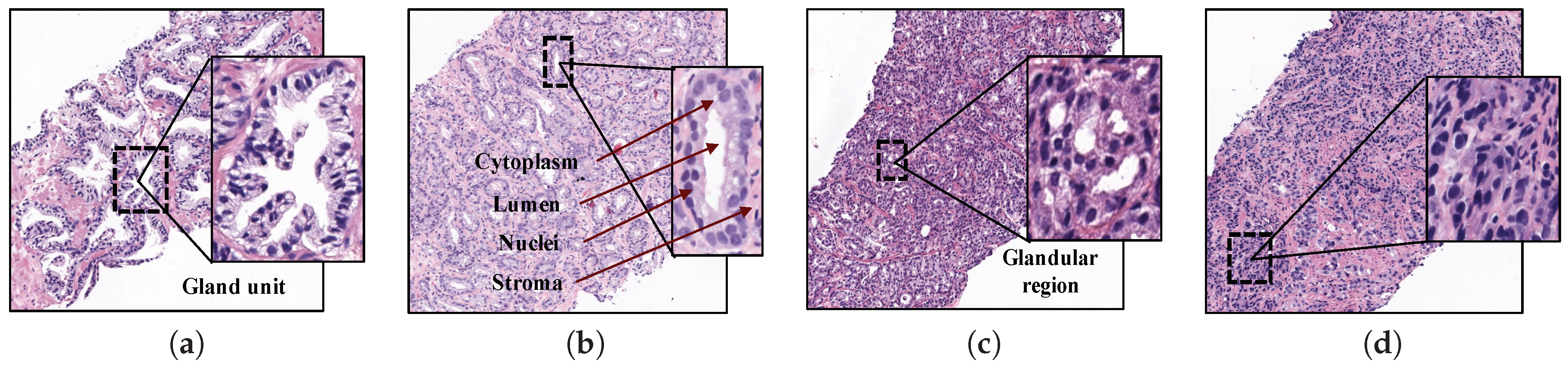
2. Materials
3. Methods
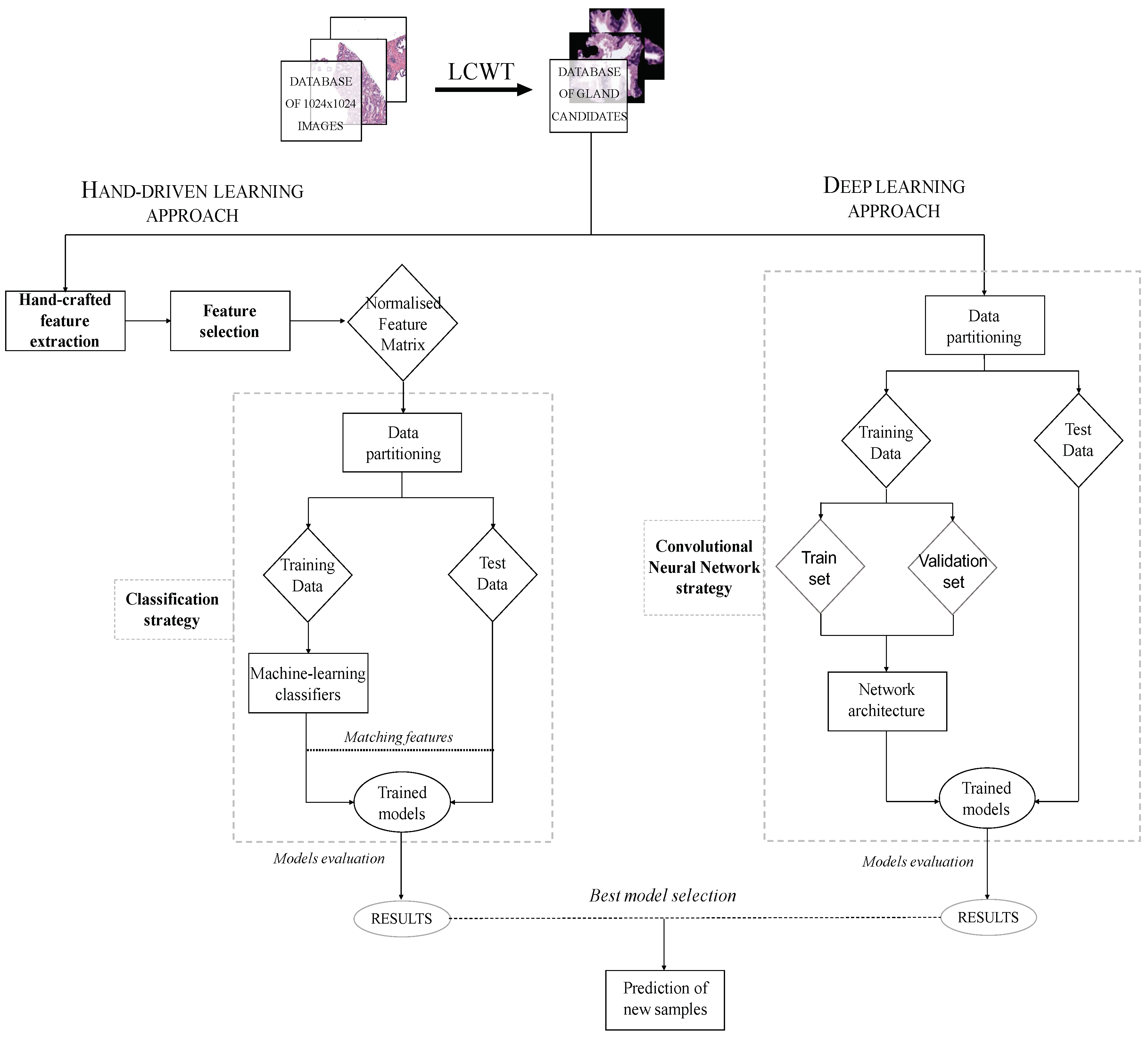
3.1. Flowchart
3.2. Background
3.3. Hand-Driven Learning Approach
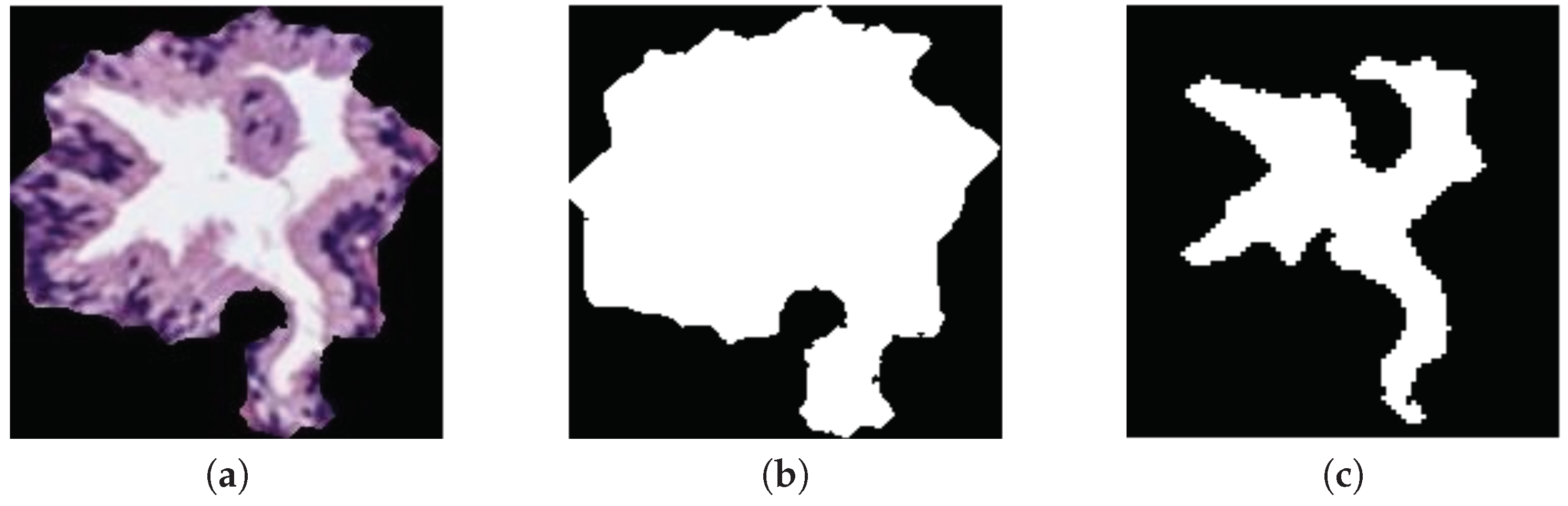
3.3.1. Feature Extraction
- . Number of pixels that contain a certain gland candidate.
- . Number of pixels in the region known as convex hull that are defined by the smallest convex polygon around the gland.
- . Ratio of the distance between the centre of and its major axis length, where is the ellipse adjusted to the gland area with their same second moments.
- . Diameter of a circle with the same area as the gland, defined by: .
- . Ratio of pixels between and the area of the bounding box that contains the gland. It is computed as follows: .
- . Angle between the x-axis and the major axis of .
- . Number of pixels that describe the edge of the gland.
- . Proportion of the pixels in the convex hull also included inside the area of the gland. It is described as: .
- . Scalar that measures the compact character of the gland by: , where is the radius of the gland.
- . Scalar indicating how round the gland is, according to: .
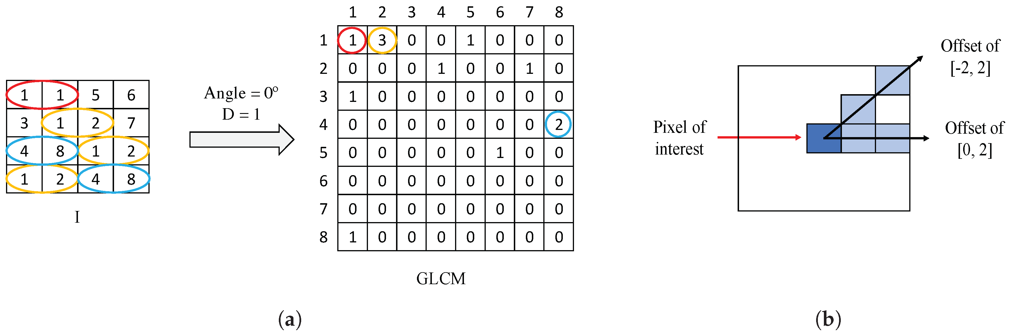
- . It reaches high values when the occurrence is focused along the normalised GLCM diagonal. Being the probability of occurrence of the grey values i and j, the homogeneity is calculated according to:
- . It measures the local variation of a certain image. It is the opposite to the homogeneity and it is computed by:
- . The energy, a.k.a. the angular second moment, takes small values when all inputs are similar. It is denoted as follows:
- . The correlation indicates how much similar information provides a pixel over the whole image regarding its neighbour. It is denoted by:
- . It is a measure related to the uniformity of image. The entropy takes small values when the inputs of are close to 0 or 1. It follows the next equation:
- . This feature corresponds to an average by columns of the grey values of the . Thus, we obtain values from columns, according to:
- . Similarly to the previous variable, here we also obtain eight values relative to the standard deviation of the calculated by columns:
- . It corresponds to the quantity of nuclei elements inside of the bounding box of the segmented gland . Being a certain individual nuclei element composed of T connected pixels with 8-connectivity, we compute:
- . We calculate the ratio relative to the number of nuclei elements and the area of the (), according to:
- . It is similar to the first variable, but, here, we calculate the number of nuclei objects inside the gland candidate area , instead of inside the area.
- . Similarly to the second feature, we also calculate the ratio of nuclei objects, but, with respect to the gland candidate area, as we expose below:
- . In this case, we compute the ratio between the number of nuclei elements inside the area gland in relation to the number of nuclei elements inside the bounding box, according to:
- . This feature makes reference to the proportion between the lumen and gland areas, in terms of number of pixels. It is computed as follows:
- . We calculate the average distance between the centroid of a lumen and the pixels of its edge, using the Euclidean distance according to:where N is the total number of pixels of the lumen edge, are the coordinates corresponding to the centroid of the lumen and the coordinates of the pixel i relative to the lumen edge.
- . We also compute the standard deviation of the distance between the centroid and the edge of each lumen, by means of:where
- . To compute this feature, first, we acquire a toroid region by subtracting the masks relative to the gland and lumen candidates, and , respectively, according to . Then, we calculate the number of pixels associated with the nuclei and cytoplasm masks, and , inside the toroid region, as follows:
- . It corresponds to the ratio between the number of pixels of the cytoplasm and nuclei masks inside the with respect to the area of such region . It is defined by:
3.3.2. Feature Selection
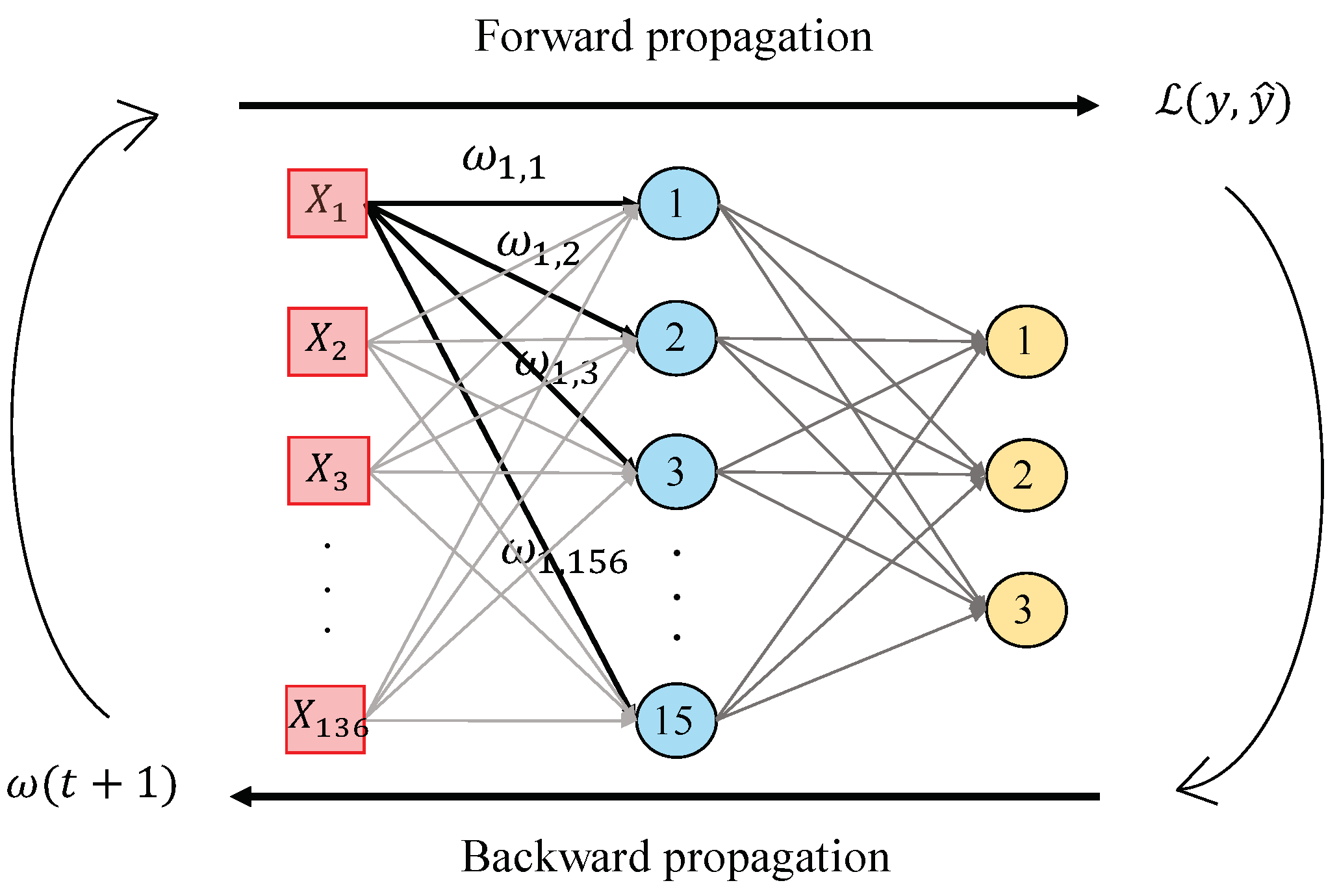
3.3.3. Classification Strategy
3.4. Deep-Learning Approach
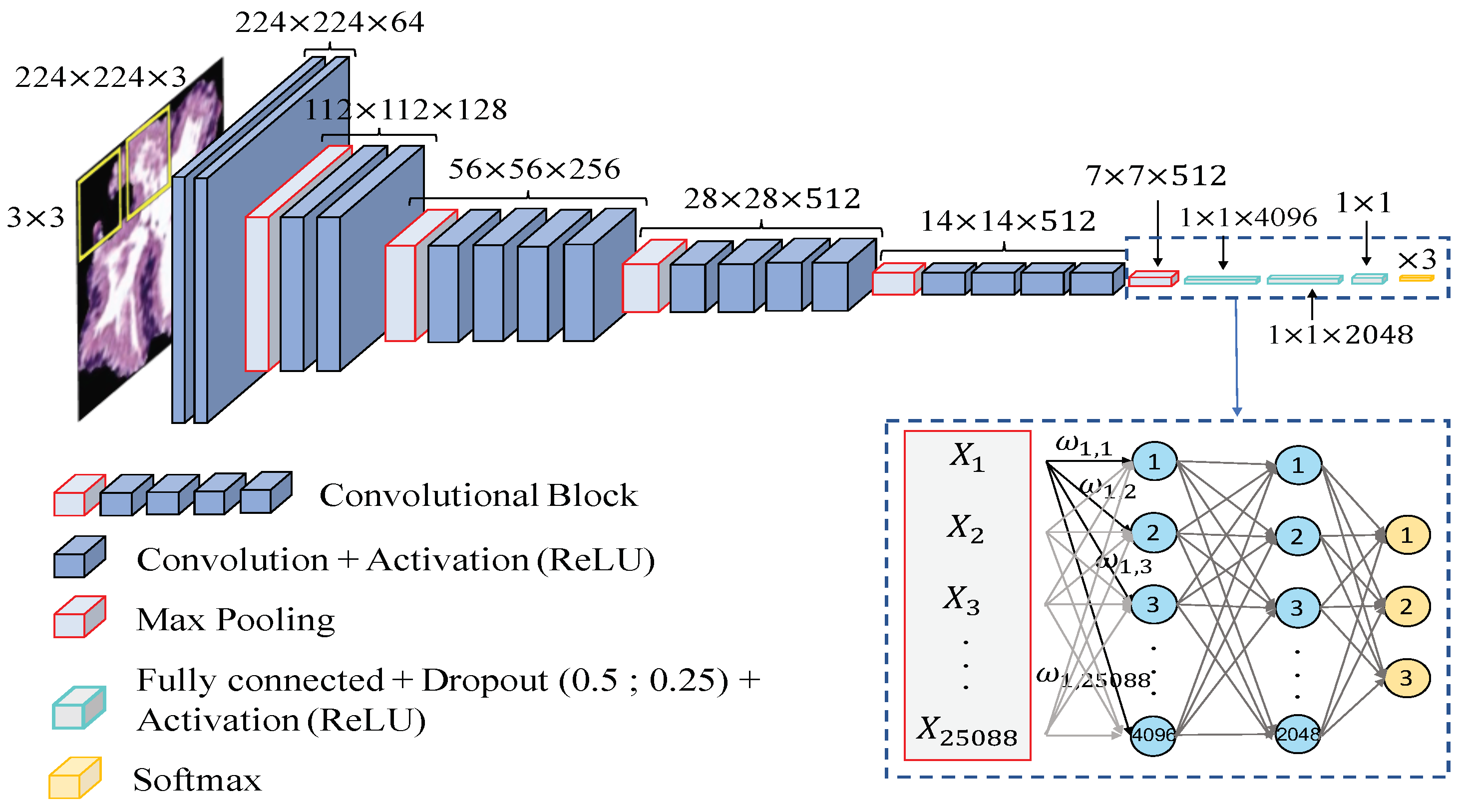
Convolutional Neural Network Strategy
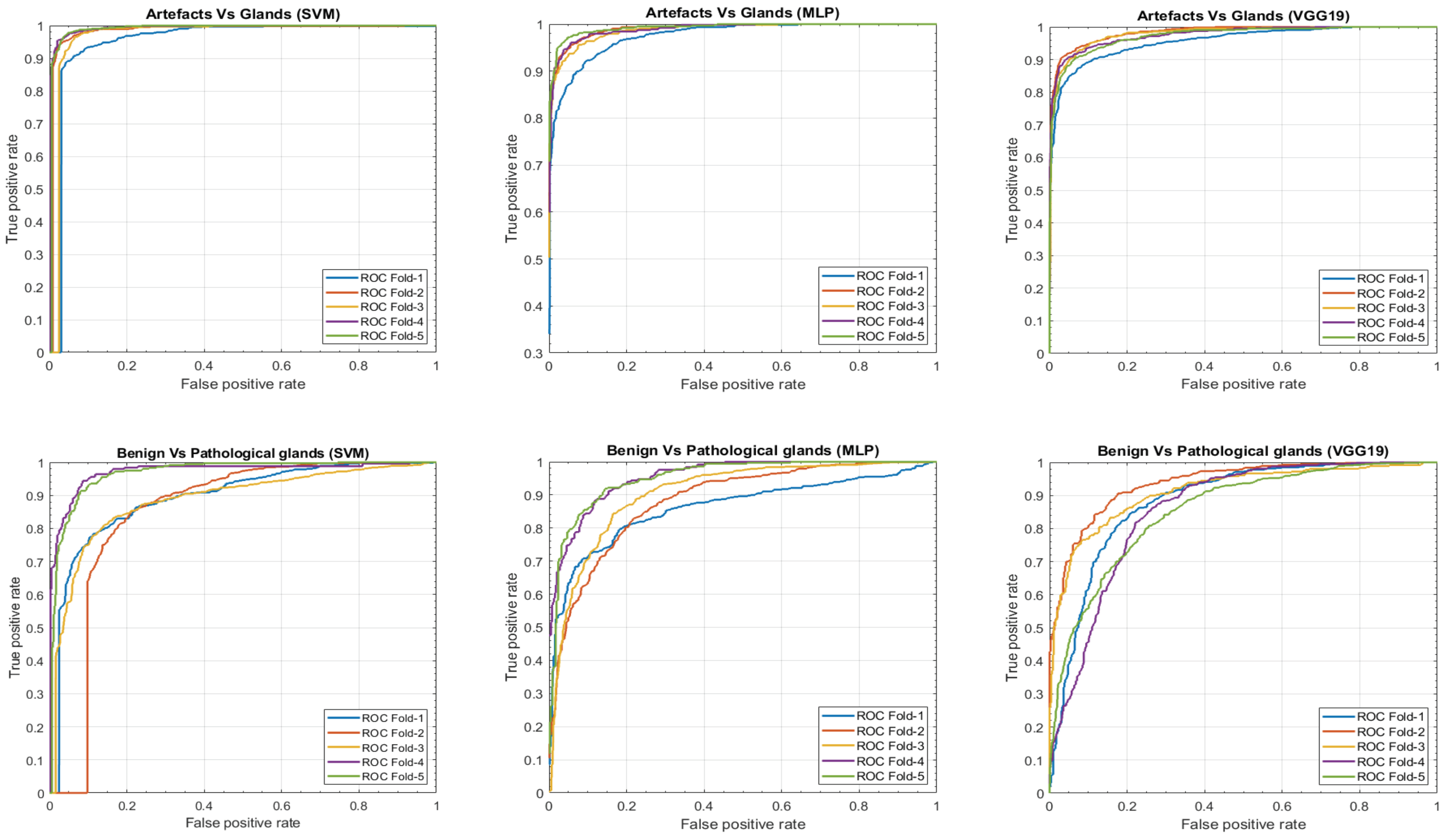
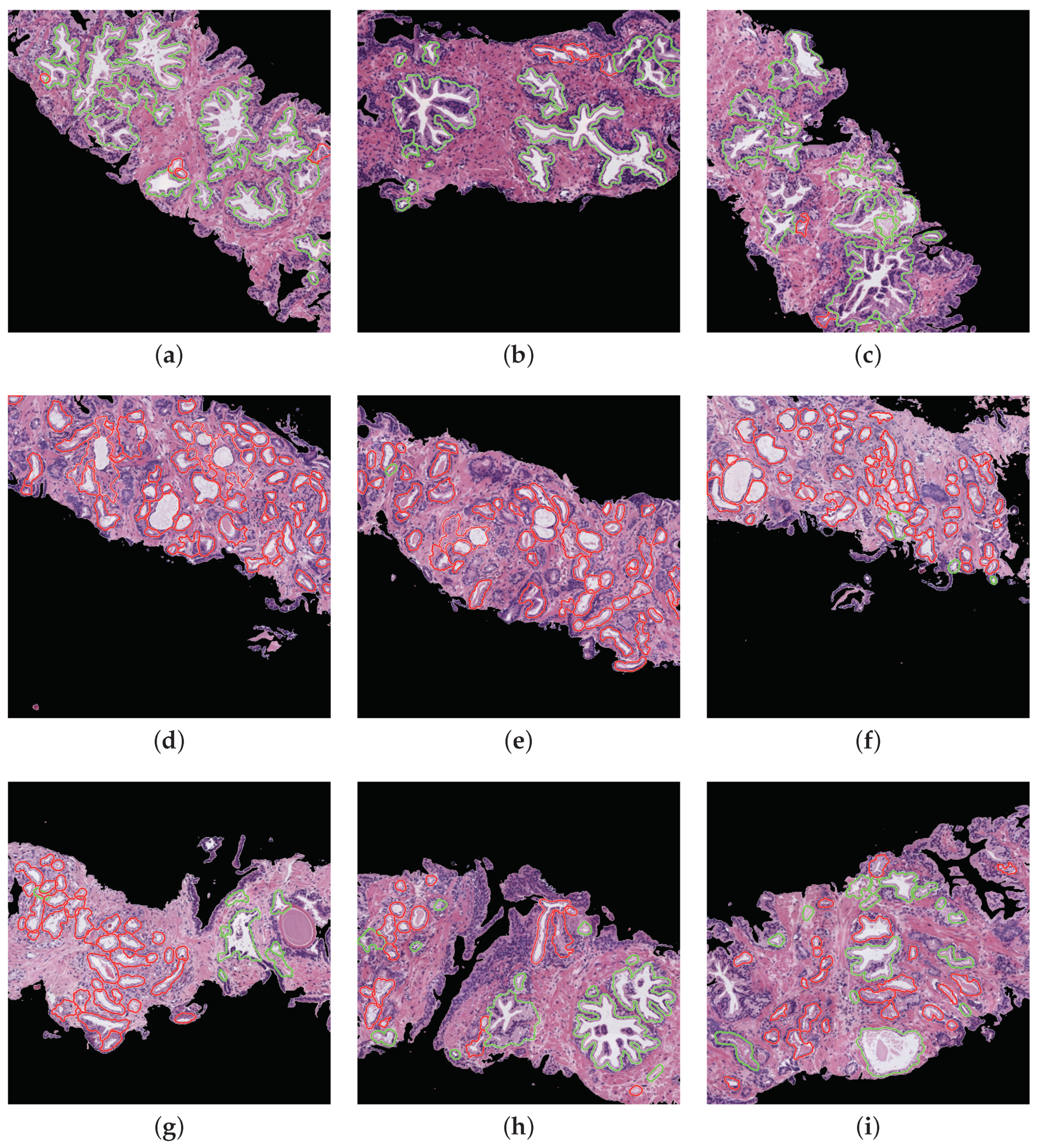
4. Results
5. Discussion
6. Conclusions
Author Contributions
Funding
Acknowledgments
Conflicts of Interest
References
- Siegel, R.L.; Miller, K.D.; Jemal, A. Cancer statistics, 2019. CA A Cancer J. Clin. 2019, 69. [Google Scholar] [CrossRef] [PubMed]
- SEOM. Las cifras del cáncer en España. 2018. Available online: https://seom.org/seomcms/images/stories/recursos/Las_Cifras_del_cancer_en_Espana2018.pdf (accessed on 25 October 2018).
- Gleason, D. Histologic grading and clinical staging of prostatic carcinoma. In Urologic Pathology: The Prostate; Lea & Febiger: Philadelphia, PA, USA, 1977; Volume 171, pp. 171–198. [Google Scholar]
- Naik, S.; Doyle, S.; Feldman, M.; Tomaszewski, J.; Madabhushi, A. Gland segmentation and computerized gleason grading of prostate histology by integrating low-, high-level and domain specific information. In MIAAB Workshop; Citeseer: Piscataway, NJ, USA, September 2007; pp. 1–8. [Google Scholar]
- Tabesh, A.; Teverovskiy, M.; Pang, H.Y.; Kumar, V.P.; Verbel, D.; Kotsianti, A.; Saidi, O. Multifeature prostate cancer diagnosis and Gleason grading of histological images. IEEE Trans. Med. Imaging 2007, 26, 1366–1378. [Google Scholar] [CrossRef]
- Nguyen, K.; Sabata, B.; Jain, A.K. Prostate cancer grading: Gland segmentation and structural features. Pattern Recognit. Lett. 2012, 33, 951–961. [Google Scholar] [CrossRef]
- Farooq, M.T.; Shaukat, A.; Akram, U.; Waqas, O.; Ahmad, M. Automatic gleason grading of prostate cancer using Gabor filter and local binary patterns. In Proceedings of the 2017 40th International Conference on Telecommunications and Signal Processing (TSP), Barcelona, Spain, 5–7 July 2017; pp. 642–645. [Google Scholar]
- Farjam, R.; Soltanian-Zadeh, H.; Jafari-Khouzani, K.; Zoroofi, R.A. An image analysis approach for automatic malignancy determination of prostate pathological images. Cytom. Part B Clin. Cytom. 2007, 72, 227–240. [Google Scholar] [CrossRef] [PubMed]
- Kwak, J.T.; Hewitt, S.M. Multiview boosting digital pathology analysis of prostate cancer. Comput. Methods Programs Biomed. 2017, 142, 91–99. [Google Scholar] [CrossRef]
- Esteban, Á.; Colomer, A.; Naranjo, V.; Sales, M. Granulometry-Based Descriptor for Pathological Tissue Discrimination in Histopathological Images. In Proceedings of the 2018 25th IEEE International Conference on Image Processing (ICIP), Athens, Greece, 7–10 October 2018; pp. 1413–1417. [Google Scholar]
- Diamond, J.; Anderson, N.H.; Bartels, P.H.; Montironi, R.; Hamilton, P.W. The use of morphological characteristics and texture analysis in the identification of tissue composition in prostatic neoplasia. Hum. Pathol. 2004, 35, 1121–1131. [Google Scholar] [CrossRef]
- Tai, S.K.; Li, C.Y.; Wu, Y.C.; Jan, Y.J.; Lin, S.C. Classification of prostatic biopsy. In Proceedings of the 2010 6th International Conference on Digital Content, Multimedia Technology and its Applications (IDC), Seoul, Korea, 16–18 August 2010; pp. 354–358. [Google Scholar]
- Doyle, S.; Hwang, M.; Shah, K.; Madabhushi, A.; Feldman, M.; Tomaszeweski, J. Automated grading of prostate cancer using architectural and textural image features. In Proceedings of the 4th IEEE International Symposium on Biomedical Imaging: From Nano to Macro, Arlington, VA, USA, 12–15 April 2007; pp. 1284–1287. [Google Scholar]
- Arvaniti, E.; Fricker, K.S.; Moret, M.; Rupp, N.J.; Hermanns, T.; Fankhauser, C.; Wey, N.; Wild, P.J.; Rüschoff, J.H.; Claassen, M. Automated Gleason grading of prostate cancer tissue microarrays via deep learning. Sci. Rep. 2018, 8, 280024. [Google Scholar] [CrossRef]
- Leo, P.; Elliott, R.; Shih, N.N.; Gupta, S.; Feldman, M.; Madabhushi, A. Stable and discriminating features are predictive of cancer presence and Gleason grade in radical prostatectomy specimens: A multi-site study. Sci. Rep. 2018, 8, 14918. [Google Scholar] [CrossRef]
- Nguyen, K.; Sarkar, A.; Jain, A.K. Structure and context in prostatic gland segmentation and classification. In Proceedings of the International Conference on Medical Image Computing and Computer-Assisted Intervention, Nice, France, 1–5 October 2012; Springer: Berlin/Heidelberg, Germany, 2012; pp. 115–123. [Google Scholar]
- Xia, T.; Yu, Y.; Hua, J. Automatic detection of malignant prostatic gland units in cross-sectional microscopic images. In Proceedings of the 2010 17th IEEE International Conference on Image Processing (ICIP), Hong Kong, China, 26–29 September 2010; pp. 1057–1060. [Google Scholar]
- García, J.G.; Colomer, A.; Naranjo, V.; Sales, M.; García-Morata, F. Comparación de estrategias de machine learning cásico y de deep learning para la clasificación automática de estructuras glandulares en imágenes histológicas de próstata. In Proceedings of the XXXVI Congreso Anual de la Sociedad Española de Ingeniería Biomédica (CASEIB), Ciudad Real, Spain, 21–23 November 2018; pp. 357–360. [Google Scholar]
- Beare, R. A locally constrained watershed transform. IEEE Trans. Pattern Anal. Mach. Intell. 2006, 28, 1063–1074. [Google Scholar] [CrossRef]
- García, J.G.; Colomer, A.; Naranjo, V.; Peñaranda, F.; Sales, M. Identification of Individual Glandular Regions Using LCWT and Machine Learning Techniques. In Proceedings of the International Conference on Intelligent Data Engineering and Automated Learning, Madrid, Spain, 21–23 November 2018; Springer: Cham, Switzerland, 2018; pp. 642–650. [Google Scholar]
- Monaco, J.P.; Tomaszewski, J.E.; Feldman, M.D.; Hagemann, I.; Moradi, M.; Mousavi, P.; Boag, A.; Davidson, C.; Abolmaesumi, P.; Madabhushi, A. High-throughput detection of prostate cancer in histological sections using probabilistic pairwise Markov models. Med. Image Anal. 2010, 14, 617–629. [Google Scholar] [CrossRef]
- Huang, P.W.; Lee, C.H. Automatic classification for pathological prostate images based on fractal analysis. IEEE Trans. Med. Imaging 2009, 28, 1037–1050. [Google Scholar] [CrossRef] [PubMed]
- Zhou, N.; Fedorov, A.; Fennessy, F.; Kikinis, R.; Gao, Y. Large scale digital prostate pathology image analysis combining feature extraction and deep neural network. arXiv, 2017; arXiv:1705.02678. [Google Scholar]
- Del Toro, O.J.; Atzori, M.; Otálora, S.; Andersson, M.; Eurén, K.; Hedlund, M.; Rönnquist, P.; Müller, H. Convolutional neural networks for an automatic classification of prostate tissue slides with high-grade Gleason score. In Medical Imaging 2017: Digital Pathology; International Society for Optics and Photonics: Bellingham, WA, USA, 2017; Volume 10140, p. 101400O. [Google Scholar]
- Database of prostate gland candidates. Available online: https://cvblab.synology.me/PublicDatabases/ProstateGlandDB.zip (accessed on 1 April 2019).
- Resulting proposed code. Available online: https://github.com/cvblab/First-stage_cancer_detection_Entropy (accessed on 1 April 2019).
- Otsu, N. A threshold selection method from gray-level histograms. IEEE Trans. Syst. Man Cybern. 1979, 9, 62–66. [Google Scholar] [CrossRef]
- Hurst, H.E. Long Term Storage: An Experimental Study; Constable: London, UK, 1965. [Google Scholar]
- Ruifrok, A.C.; Johnston, D.A. Quantification of histochemical staining by color deconvolution. Anal. Quant. Cytol. Histol. 2001, 23, 291–299. [Google Scholar]
- Gertych, A.; Ing, N.; Ma, Z.; Fuchs, T.J.; Salman, S.; Bhele, S.; Velásquez-Vacca, A.; Amin, M.B.; Knudsen, B.S. Machine learning approaches to analyze histological images of tissues from radical prostatectomies. Comput. Med. Imaging Graphics 2015, 46, 197–208. [Google Scholar] [CrossRef]
- Mandelbrot, B.B.; Van Ness, J.W. Fractional Brownian motions, fractional noises and applications. SIAM Rev. 1968, 10, 422–437. [Google Scholar] [CrossRef]
- DiFranco, M.; O’Hurley, G.; Kay, E.; Watson, W.; Cunningham, P. Automated gleason scoring of prostatic histopathology slides using multi-channel co-occurrence texture features. In Proceedings of the International Workshop on Microscopic Image Analysis with Applications in Biology (MIAAB), New York, NY, USA, 5 September 2008. [Google Scholar]
- Presutti, M. La matriz de co-ocurrencia en la clasificación multiespectral: tutorial para la enseñanza de medidas texturales en cursos de grado universitario. In Proceedings of the 4a Jornada de Educação em Sensoriamento Remoto no Âmbito do Mercosul, São Leopoldo, RS, Brasil, 11–13 August 2004. [Google Scholar]
- Ojala, T.; Pietikäinen, M.; Harwood, D. A comparative study of texture measures with classification based on featured distributions. Pattern Recognit. 1996, 29, 51–59. [Google Scholar] [CrossRef]
- Ojala, T.; Pietikainen, M.; Maenpaa, T. Multiresolution gray-scale and rotation invariant texture classification with local binary patterns. IEEE Trans. Pattern Anal. Mach. Intell. 2002, 24, 971–987. [Google Scholar] [CrossRef]
- Pietikäinen, M.; Ojala, T.; Xu, Z. Rotation-invariant texture classification using feature distributions. Pattern Recognit. 2000, 33, 43–52. [Google Scholar] [CrossRef]
- Guo, Z.; Zhang, L.; Zhang, D. A completed modeling of local binary pattern operator for texture classification. IEEE Trans. Image Process. 2010, 19, 1657–1663. [Google Scholar]
- Chang, C.C.; Lin, C.J. LIBSVM: A library for support vector machines. ACM Trans. Intell. Syst. Technol. (TIST) 2011, 2, 27. [Google Scholar] [CrossRef]
- Bishop, C.M. Pattern Recognition and Machine Learning; Technical Report; Springer: Heidelberg/Berlin, Germany, 2006. [Google Scholar]
- Krizhevsky, A.; Sutskever, I.; Hinton, G.E. Imagenet classification with deep convolutional neural networks. In Advances in Neural Information Processing Systems; Curran Associates Inc.: Lake Tahoe, NV, USA, 2012; pp. 1097–1105. [Google Scholar]
- ImageNet Large Scale Visual Recognition Competition. Available online: www.image-net.org/challenges/LSVRC (accessed on 1 April 2019).
- Simonyan, K.; Zisserman, A. Two-stream convolutional networks for action recognition in videos. In Proceedings of the Advances in Neural Information Processing Systems 27 (NIPS 2014), Montreal, QC, Canada, 8–13 December 2014; pp. 568–576. [Google Scholar]
- Download Images of ImageNet Database. Available online: www.image-net.org/download-images (accessed on 1 April 2019).
- Hoo-Chang, S.; Roth, H.R.; Gao, M.; Lu, L.; Xu, Z.; Nogues, I.; Yao, J.; Mollura, D.; Summers, R.M. Deep convolutional neural networks for computer-aided detection: CNN architectures, dataset characteristics and transfer learning. IEEE Trans. Med. Imaging 2016, 35, 1285. [Google Scholar]
- Tajbakhsh, N.; Shin, J.Y.; Gurudu, S.R.; Hurst, R.T.; Kendall, C.B.; Gotway, M.B.; Liang, J. Convolutional neural networks for medical image analysis: Full training or fine tuning? IEEE Trans. Med. Imaging 2016, 35, 1299–1312. [Google Scholar] [CrossRef] [PubMed]
- Wong, S.C.; Gatt, A.; Stamatescu, V.; McDonnell, M.D. Understanding data augmentation for classification: When to warp? In Proceedings of the 2016 International Conference on Digital Image Computing: Techniques and Applications (DICTA), Gold Coast, QLD, Australia, 30 November–2 December 2016; pp. 1–6. [Google Scholar]


| Morphological features (13) | Gland (6) | , , , , , |
| Lumen (7) | , , , , , , | |
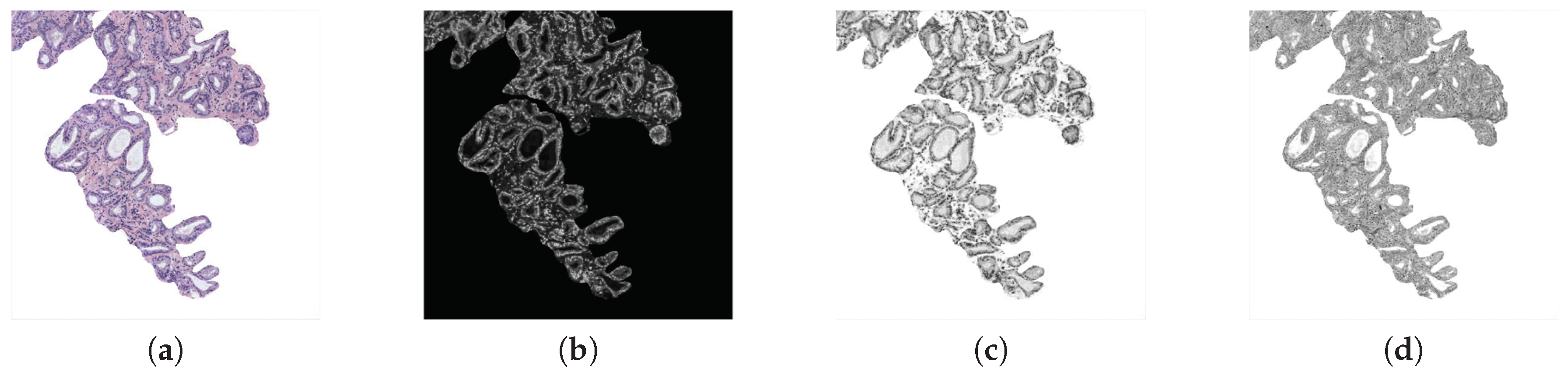
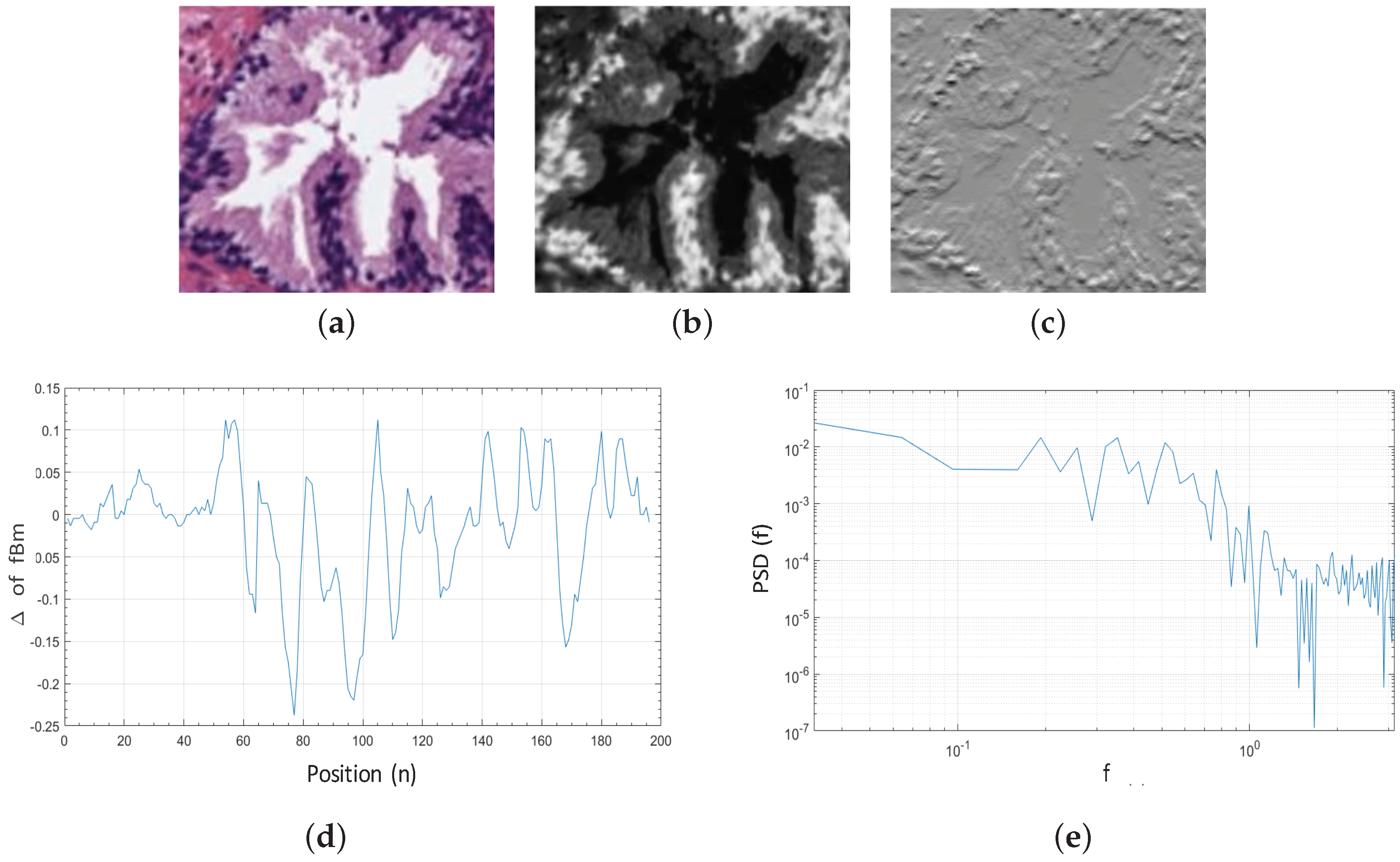
| Fractal analysis (11) | Cyan (3) | , , |
| Hematoxylin (5) | , , , , | |
| Eosin (3) | , , | |
| Textural features (94) | Cyan (32) | , , , , , , , , , |
| Hematoxylin (27) | , , , , , , | |
| Eosin (35) | , , , , , , , , , | |
| Contextual features (18) | Nuclei (9) | , , , , , , , , |
| Cytoplasm (5) | , , , , | |
| Lumen-Nuclei-Cytoplasm (4) | , , , |
| Artefacts vs. Glands | Benign vs. Pathological | |||||
|---|---|---|---|---|---|---|
| SVM | MLP | VGG19 | SVM | MLP | VGG19 | |
| Sensitivity | ||||||
| Specificity | ||||||
| PPV | ||||||
| NPV | ||||||
| F-Score | ||||||
| AUC | ||||||
| Accuracy | ||||||
| Xia et al. [17] | Nguyen et al. [16] | Proposed Model | |
|---|---|---|---|
| Artefacts vs. Glands | - | ||
| Benign vs. Pathological | |||
| Multi-class classification | - |
| Artefact | Benign Gland | Pathological Gland | |
|---|---|---|---|
| SVM | |||
| MLP | |||
| VGG19 |
| Healthy Tissues (s) | Cancerous Tissues (s) | |
|---|---|---|
| Clustering stage | ||
| Gland segmentation | ||
| Feature extraction | ||
| Prediction | ||
| End-to-end algorithm |
© 2019 by the authors. Licensee MDPI, Basel, Switzerland. This article is an open access article distributed under the terms and conditions of the Creative Commons Attribution (CC BY) license (http://creativecommons.org/licenses/by/4.0/).
Share and Cite
García, G.; Colomer, A.; Naranjo, V. First-Stage Prostate Cancer Identification on Histopathological Images: Hand-Driven versus Automatic Learning. Entropy 2019, 21, 356. https://doi.org/10.3390/e21040356
García G, Colomer A, Naranjo V. First-Stage Prostate Cancer Identification on Histopathological Images: Hand-Driven versus Automatic Learning. Entropy. 2019; 21(4):356. https://doi.org/10.3390/e21040356
Chicago/Turabian StyleGarcía, Gabriel, Adrián Colomer, and Valery Naranjo. 2019. "First-Stage Prostate Cancer Identification on Histopathological Images: Hand-Driven versus Automatic Learning" Entropy 21, no. 4: 356. https://doi.org/10.3390/e21040356
APA StyleGarcía, G., Colomer, A., & Naranjo, V. (2019). First-Stage Prostate Cancer Identification on Histopathological Images: Hand-Driven versus Automatic Learning. Entropy, 21(4), 356. https://doi.org/10.3390/e21040356