1. Introduction
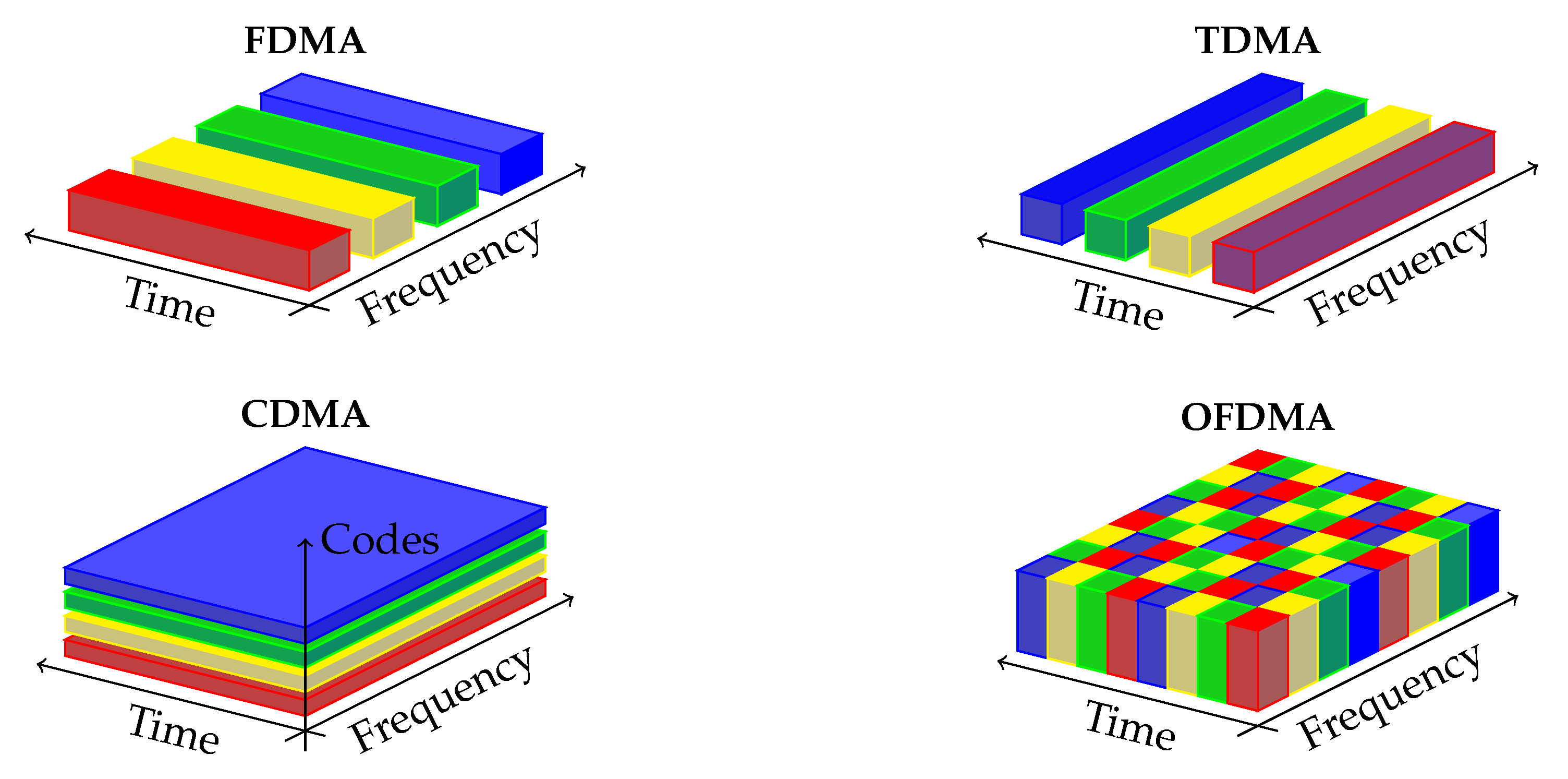
Cellular communication systems are designed to allow multiple users to share the same communication medium. Traditionally, mobile networks have enabled this feature by dividing the physical resources (such as time, frequency, code, and space) in an orthogonal manner between users. An illustration of the typical methods, called Orthogonal Multiuser Access (OMA) is shown in
Figure 1.
The future of cellular communications is facing exponential growth in bandwidth demand. Furthermore, increased popularity in Internet of Things (IoT) applications and the emergence of Vehicle-to-Vehicle (V2V) connectivity will further grow the number of network consumers. Hence, fifth-generation (5G) wireless networks are required to support extensive connectivity, low latency, and higher data rates. Such requirements cannot be satisfied using the traditional OMA methods and thus to sustain more users and higher transmission rates, non-orthogonal multiuser access (NOMA) has been intensively investigated, where interference mitigation is the key issue for non-orthogonal transmission. A comprehensive survey on NOMA from an information theoretic perspective is given in [
1].
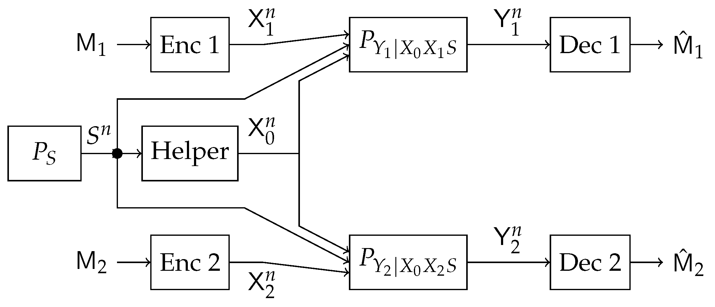
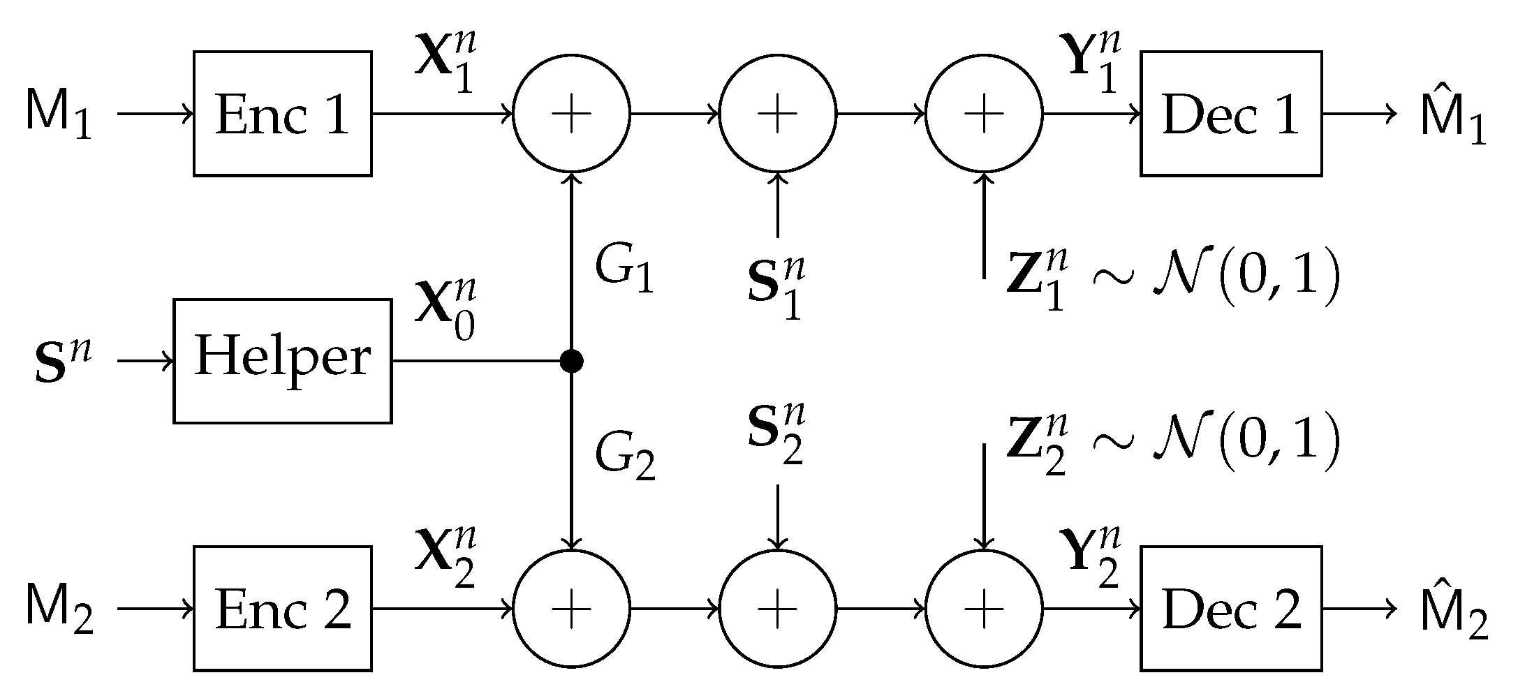
In this work, we study a particular communication model that can be used in future NOMA techniques. Specifically, we investigate a type of state-dependent channel with a helper, illustrated in
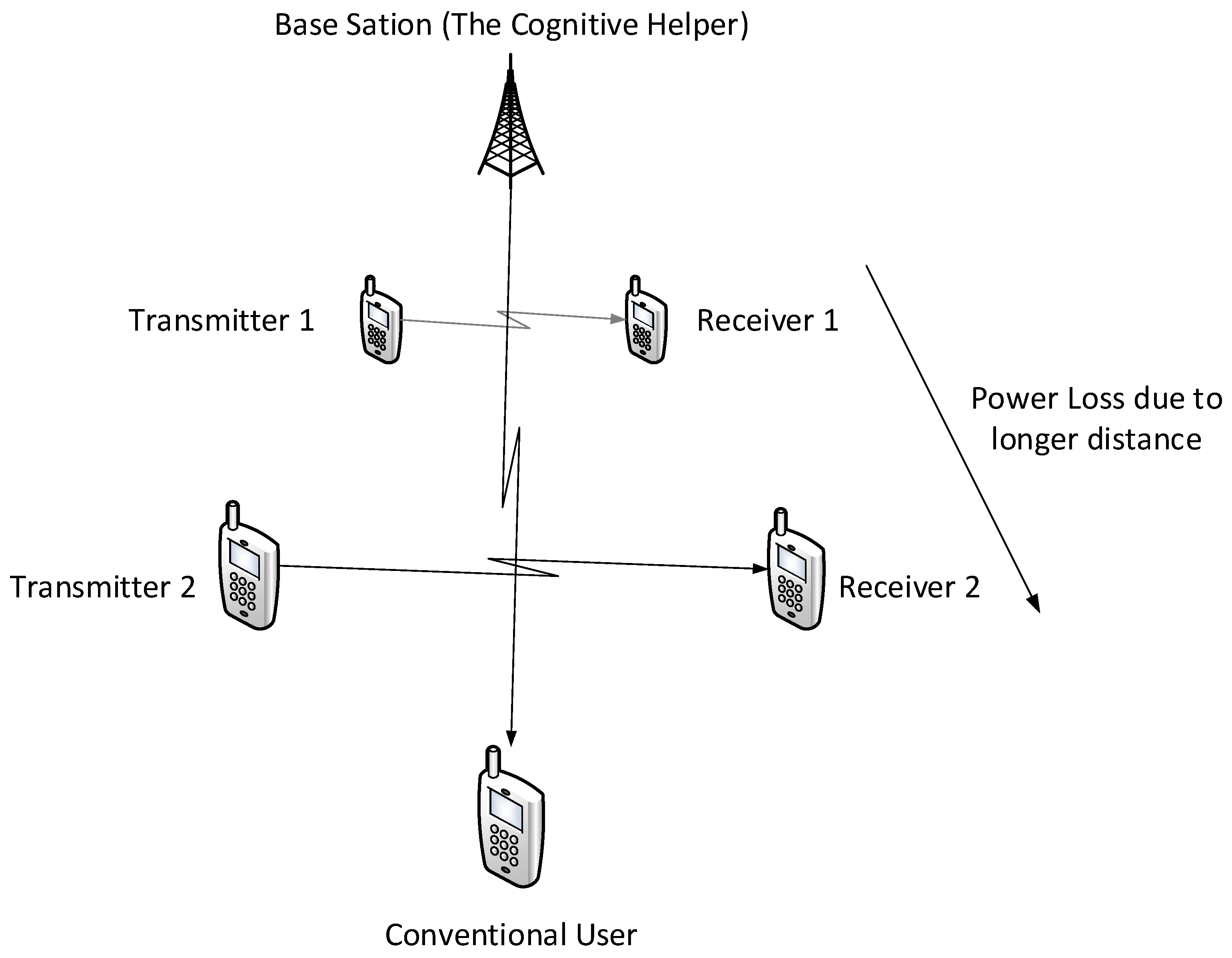
Figure 2, in which two transmitters wish to send messages to their corresponding receivers over a parallel state-dependent channel. The state is not known to either transmitter or receiver but is non-causally (the side information in all times is given to the encoder before the block transmission) known to a state-cognitive helper, who tries to assist each receiver in mitigating the interference caused by the state. This model captures interference cancelation in various practical scenarios. For example, users in multi-cell systems may be interfered by a base station located in other cells. Such a base station, being as the source that causes the interference, clearly knows the information of the interference (modeled by state) and can serve as a helper to mitigate the interference. Alternatively, that base station can also convey the interference information to other base stations via the backhaul network so that other base stations can serve as helpers to reduce the interference. As another example, consider a situation where there are two Device to Device (D2D) links located in two distinct cells, and there is a downlink signal sent from the base station to some conventional mobile user in the cell. Also, there is some central unit that knows in a non-causal manner the signal to be sent by each base station, the helper in our model, and tries to assist the D2D communication links by mitigating the interference (see
Figure 3). As a comparison, this type of state-dependent models differs from the original state-dependent channels studied in, e.g., [
2,
3], in that the state-cognitive helper is not informed of the transmitters’ messages, and hence its state cancelation strategies are necessarily independent of message encoding at the transmitters.
The study of channel coding in the presence of channel side information (CSI) was initiated by Shannon [
4] who considered a discrete memoryless channel (DMC) channel with random parameters and side information provided causally to the transmitter. The single-letter expression for the capacity of the point-to-point DMC with non-causal CSI at the encoder (the G-P channel) was derived in the seminal work of Gel’fand and Pinsker [
2]. One of the most interesting special cases of the G-P channel is the Gaussian additive noise and interference setting in which the additive interference plays the role of the state sequence, which is known non-causally to the transmitter. Costa showed in [
3] that the capacity of this channel is equal to the capacity of the same channel without additive interference. The capacity achieving scheme of [
3] (which is that of [
2] applied to the Gaussian case) is termed “writing on dirty paper” (WDP), and consequently, the property of the channel where the known interference can be completely removed is dubbed “the WDP property”. Cohen and Lapidoth [
5] showed that any interference sequence can be removed entirely when the channel noise is ergodic and Gaussian.
The models we study in this work all have a broadcasting node. The
discrete memoryless broadcast channel (DM-BC) was introduced by Cover [
6]. The capacity region of the DM-BC is still an open problem. The largest known inner bound on the capacity region of the DM-BC with private messages was derived by Marton [
7]. Liang [
8] derived an inner bound on the capacity region of the DM-BC with an additional common message. The best outer bound for DM-BC with a common message is due to Nair and El Gamal [
9]. There are, however, some special cases where the capacity region is fully characterized. For example, the capacity region of the degraded DM-BC was established by Gallager [
10]. The capacity region of the Gaussian BC was derived by Bergmans [
11]. An interesting result is the capacity region of the Gaussian MIMO BC which was established by Weingarten et al. [
12]. The authors introduced a new notion of
an enhanced channel and used it jointly with the Entropy Power Inequality (EPI) to show their result. The capacity achieving scheme relies on the dirty paper coding technique. Liu and Viswanath [
13] developed
an extremal inequality proof technique and showed that it can be used to establish a converse result in various Gaussian MIMO multiterminal networks, including the Gaussian MIMO BC with private messages. Recently, Geng and Nair [
14] developed a different technique to characterize the capacity region of Gaussian MIMO BC with common and private messages.
Degraded DM-BC with causal and non-causal side information was introduced by Steinberg [
15]. Inner and outer bounds on the capacity region were derived. For the particular case in which the nondegraded user is informed about the channel parameters, it was shown that the bounds are tight, thus obtaining the capacity region for that case. The general DM-BC with non-causal CSI at the encoder was studied by Steinberg and Shamai [
16]. An inner bound was derived, and it was shown to be tight for the Gaussian BC with private messages and independent additive interference at both channels. The latter setting was recently extended to the case of common and private messages in the Gaussian framework with
K users in [
17]. The special case where the transmitter sends only a common message to all receivers over an additive BC has been initially studied in [
18] and has been recently extended to the compound setting in [
19]. Outer bounds for DM-BC with CSI at the encoder were derived in [
20].
The models addressed in this paper have a mismatched property, that is the state sequence is known only to some nodes, which differs from the classical study on state-dependent channels. The type of channels with mismatched property has been addressed in the past for various models, for example, in [
21,
22,
23,
24,
25], the state-dependent
multiple access channel (MAC) is studied with the state known at only one transmitter. The best outer bound for the Gaussian MAC setting was recently reported in [
26]. The point-to-point helper channel studied in [
27,
28] can be considered as a special case of [
25], where the cognitive transmitter does not send any message. Further in [
28], the state-dependent MAC with an additional helper was studied, and the partial/full capacity region was characterized under various channel parameters. Moreover, some state-dependent relay channel models can also be viewed as an extension of the state-dependent channel with a helper, where the relay serves the role of the helper by knowing the state information. In [
29], the state-dependent relay channel with state non-causally available at the relay is considered. An achievable rate was derived using a combination of decode-and-forward, Gel`fand–Pinsker (GP) binning and codeword splitting. Also, in [
30], additional noiseless cooperation links with finite capacity were assumed between the transmitter and the relay, and various coding techniques were explored. The authors of [
31] have recently considered a different scenario with a state-cognitive relay. The state-dependent Z-IC with a common state known in a non-causal manner only to the primary user was studied in [
32]. A good tutorial on channel coding in the presence of CSI can be found in [
33].
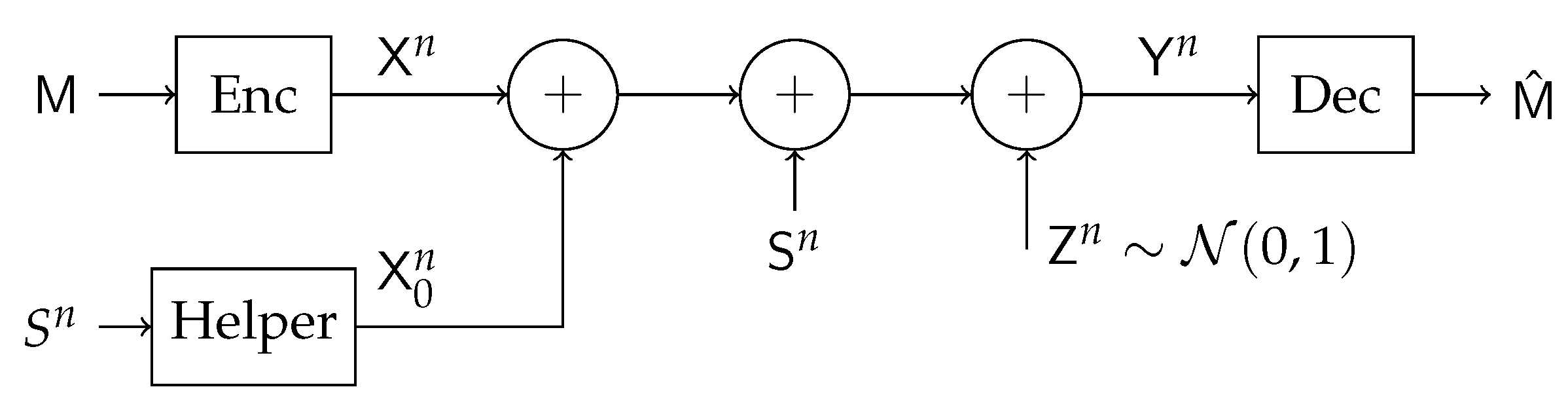
The basic state-dependent Gaussian channel with a helper is illustrated in
Figure 4. It was first introduced in [
27], where the capacity in the infinite power regime was characterized and was shown to be achievable by lattice coding. The capacity under arbitrary state power was established for some special cases in [
28]. Based on a single-bin GP binning scheme the following lower bound was derived for the discrete memoryless case
This lower bound was further evaluated for Gaussian channel by appropriate choice of the maximizing input distribution. The surprising result of that study was that when the helper power is above some threshold, then the interference caused by the state is entirely canceled and the capacity of the channel without the state can be achieved. This threshold does not depend on the state power, and hence it was shown that this channel also has WDP property, that is the capacity of the channel is the same as the capacity of the similar channel without the interference (which is modeled as the state).
The most relevant work to this study is [
34], in which the state-dependent parallel channel with a helper was studied, for the regime with infinite state power and with two receivers being corrupted by two independent states. A time-sharing scheme was proved to be capacity achieving under certain channel parameters. In contrast, in this study, we expand those results for the arbitrary state power regime. We also consider two extreme cases. At first, we address the problem where the two receivers of the parallel channel are corrupted by the same but differently scaled states, and in the second part, those states are independent. For both cases, we show that the time-sharing scheme is no longer optimal. Our main contribution in this work is a derivation of inner bound, which is an extension of the Marton coding scheme for the discrete broadcast channel to the current model. We will apply this bound for the MIMO Gaussian setting and characterize the segments of the capacity region for various channel parameters. The material in this paper was presented in part at [
35,
36].
3. The MIMO Gaussian Channel with Same but Differently Scaled States
3.1. Channel Model
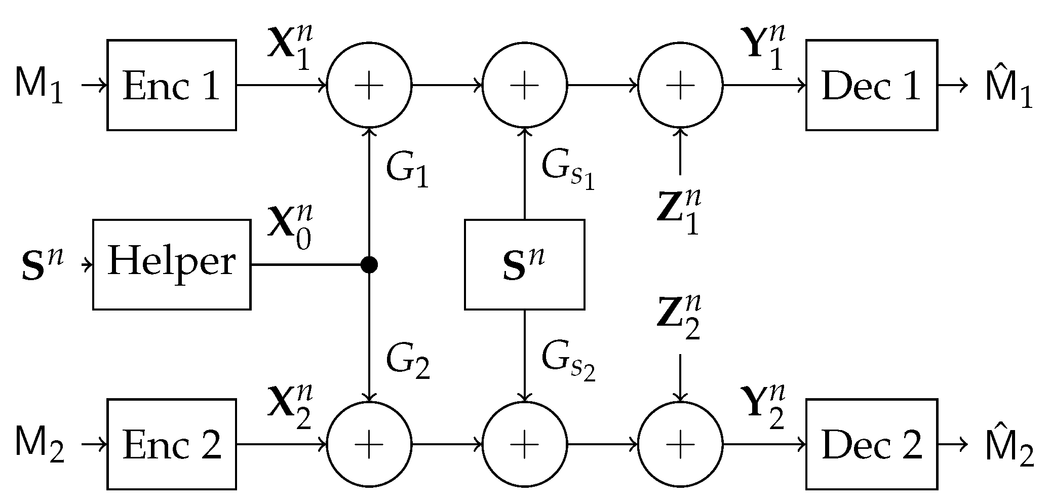
In this section, we study the state-dependent parallel network with a state-cognitive helper, in which two transmitters communicate with two corresponding receivers over a state-dependent parallel channel. The two receivers are corrupted by the same but differently scaled state, respectively. The state information is not known to either the transmitters or the receivers, but a helper non-causally. Hence, the helper assists these receivers to cancel the state interference (see
Figure 5).
More specifically, the encoder at transmitter
l,
, maps a message
to a codeword
, for
. The inputs
and
are sent respectively over the two subchannels of the parallel channel. The two receivers are corrupted by the same but differently scaled and identically distributed (i.i.d.) state sequence
, which is known to a common helper non-causally. Hence, the encoder at the helper,
, maps the state sequence
into a codeword
. The channel transition probability is given by
. The decoder at receiver
l,
, maps a received sequence
into a message
, for
. We assume that the messages are uniformly distributed over the sets
and
. We define the average probability of error for a length-
n code as
Definition 2. A rate pair is said to be achievable if there exist a sequence of message sets and , and encoder-decoder tuples such that the average probability of error as .
Definition 3. We define the capacity region of the channel as the closure of the set of all achievable rate pairs .
In this section, we focus on the MIMO Gaussian channel, with the outputs at the two receivers for one channel use given by
where
,
,
,
,
and
are all real vectors of size
, and
, , are the input vectors that are subject to the covariance matrix constraints , ,
is the output vector, ,
is a real Gaussian random vector with zero mean and covariance matrix ,
is a real Gaussian random vector with zero mean and an identity covariance matrix , for .
Both the noise variables, and the state variable are i.i.d. over channel uses. () is real matrix that represents the channel matrix connecting the state source to the first (second) user. Similarly, () is a real channel matrix connecting the helper to the first (second) user. Thus, our model captures a general scenario, where the helper’s power and the state power can be arbitrary.
Our goal is to characterize the capacity region of the Gaussian channel under various channel parameters .
3.2. Inner and Outer Bounds
In this section, we first derive inner and outer bounds on the capacity region for the state-dependent parallel channel with a helper. Then by comparing the inner and outer bounds, we characterize the segments on the capacity region boundary under various channel parameters.
We start by deriving an inner bound on the capacity region for the DMC based on the single-bin GP scheme.
Proposition 1. For the discrete memoryless state-dependent parallel channel with a helper under the same but differently scaled states at the two receivers, an inner bound on the capacity region consists of rate pairs satisfying:for some distribution . We evaluate the inner bound for the Gaussian channel by choosing the joint Gaussian distribution for random variables as follows:
where
are independent and
.
Let
and
be defined as
where the mutual information terms are evaluated using the joint Gaussian distribution chosen in (
8). Based on those definitions, we obtain an achievable region for the Gaussian channel.
Proposition 2. An inner bound on the capacity region of the parallel state-dependent MIMO Gaussian channel with same but differently scaled states and a state-cognitive helper consists of rate pairs satisfying;for some real matrices A, B and satisfying , . We note that the above choice of the helper’s signal incorporates two parts with designed using single-bin dirty paper coding, and acting as direct state subtraction.
We next present an outer bound which applies the point-to-point channel capacity and the upper bound derived for the point-to-point channel with a helper in [
27].
Proposition 3. An outer bound on the capacity region of the state-dependent parallel MIMO Gaussian channel with a helper consists of rate pairs satisfying:for every and that satisfies . Proof. The second term in (
11) is simply the capacity of a point-to-point channel without state. The first term is derived in
Appendix B. □
3.3. Capacity Region Characterization
In this section, we optimize A and B in Proposition 2, and compare the rate bounds with the outer bounds in Proposition 3 to characterize the points or segments on the capacity region boundary.
Since the inner bound in Proposition 2 is not convex, it is difficult to provide a closed form for the jointly optimized bounds. Therefore, we first optimize the bounds for and respectively, and then provide conditions on channel parameters such that these bounds match the outer bound. Based on the conditions, we partition the channel parameters into the sets, in which different segments of the capacity region boundary can be obtained.
We first consider the rate bound for
in (
9a). By setting
takes the following form
where
maximizes
. In fact,
maximizes
for fixed
B, and
maximizes the function with
.
If
,
is achievable, and this matches the outer bound in (
11). Thus, one segment of the capacity region is specified by
We further observe that the second term
in (
9a) is optimized by setting
, and hence
If
, i.e.,
then the inner bound for
becomes
, which is the capacity of the point-to-point channel without state and matches the outer bound in (
11). Thus, another segment of the capacity is specified by
We then consider the rate bound for
. Similarly, the following segments on the capacity boundary can be obtained. If
, one segment of the capacity region boundary is specified by
where
and
maximizes
.
Furthermore, if
, one segment of the capacity region boundary is specified by
Appendix C describes how
,
,
and
were chosen.
Summarizing the above analysis, we obtain the following characterization of segments of the capacity region boundary.
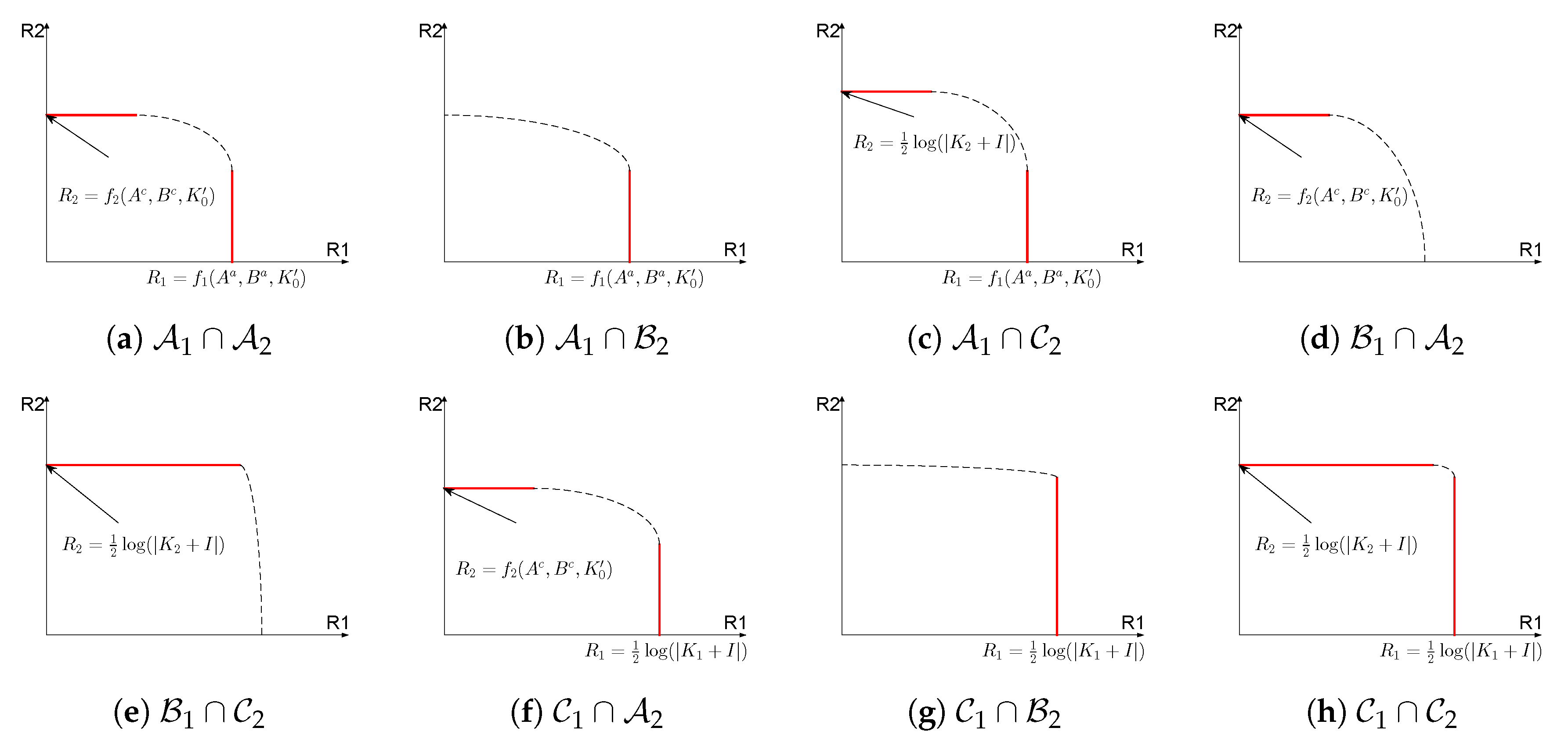
Theorem 1. The channel parameters can be partitioned into the sets , where If , then (12a)–(12b) captures one segment of the capacity region boundary, where the state cannot be fully canceled. If , then (14a)–(14b) captures one segment of the capacity region boundary where the state is fully canceled. If , then the segment of the capacity region boundary is not characterized. The channel parameters can also be partitioned into the sets , where If , then (15a)–(15b) captures one segment of the capacity region boundary, where the state cannot be fully canceled. If , then (16a)–(16b) captures one segment of the capacity boundary where the state is fully canceled. If , then the segment of the capacity region boundary is not characterized. The above theorem describes two partitions of the channel parameters, respectively under which segments on the capacity region boundary corresponding to and can be characterized. Intersection of two sets, each from one partition, collectively characterizes the entire segments on the capacity region boundary.
Figure 6 lists all possible intersection of sets that the channel parameters can belong to. For each case in
Figure 6, we use red solid line to represent the segments on the capacity region that are characterized in Theorem 1, and we also mark the value of the capacity that each segment corresponds to as characterized in Theorem 1. Please note that the case
is not illustrated in
Figure 6 since no segments are characterized in this case.
One interesting example in Theorem 1 is the case with , in which and are optimized with the same set of coefficients A and B when . Thus, the point-to-point channel capacity is simultaneously obtained for both and , with state being fully canceled. We state this result in the following theorem.
Theorem 2. If , and where , for some then the capacity region of the state-dependent parallel Gaussian channel with a helper and under the same but differently scaled states contains satisfying The channel conditions of Theorem 2 are not just of mathematical importance but also have a practical utility. Consider, for example, a scenario where the helper is also the interferer (see
Figure 3), in such case it is reasonable to assume that
and
, and thus the aforementioned conditions are satisfied.
3.4. Numerical Example
We now examine our results via simulations. In particular, we focus on the scalar channel case, i.e., , , , , , , , and . Furthermore, we denote , and .
We set
,
,
, and
, and plot the inner and outer bounds for the capacity region
for two values of
a. It can be observed from
Figure 7 that the upper bound is defined by the rectangular region of channel without state. The inner bound, in the contrary, is susceptible to the value of
a, such that in the case where
, our inner and outer bounds coincide everywhere, while in the case
they coincide only on some segments. Both observations corroborate the characterization of the capacity in Theorems 1 and 2.
It is also interesting to illustrate how the channel parameters affect our ability to characterize the capacity region boundary. For this we propose the following setup:
we choose and such that lies on the capacity region boundary;
we further choose that maximizes the achievable , denoted as ;
we compare it to the outer bound of , , and plot the gap .
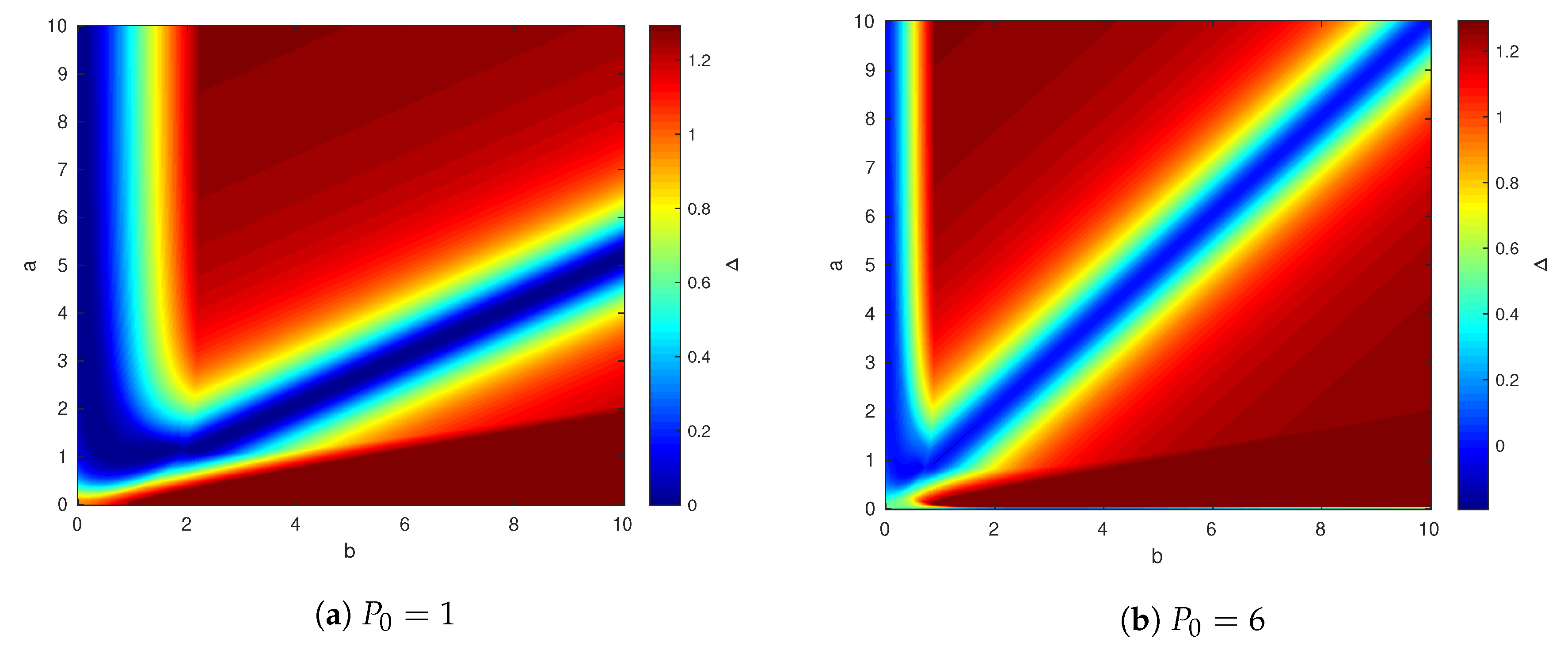
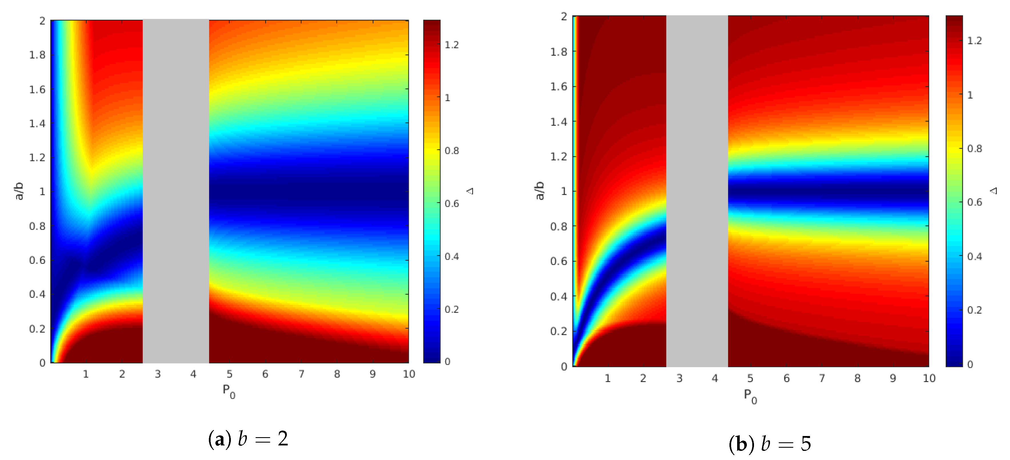
Figure 8 shows the results of such simulation for two values of
:
for which the state is not fully canceled for user 1 and
, for which the state is canceled. We fix other parameters as before, that is
and
. The right figure shows that the capacity gap is small around the line
, this result is not surprising, and it appears in Theorem 2. The left Figure is also interesting. It shows that there is a curve
for which the capacity gap is also near zero. The reason for this phenomenon is explained as follows.
The chosen channel parameters satisfy
, and hence
optimize
.
Thus, if
satisfies
and
, then
, i.e.,
is achievable.
We illustrate this result in
Figure 9, where we fixed the channel parameters
,
,
, and calculate the capacity gap for various values of
a and
. The shaded area is the region of
where the capacity of the point-to-point helper channel is not characterized.
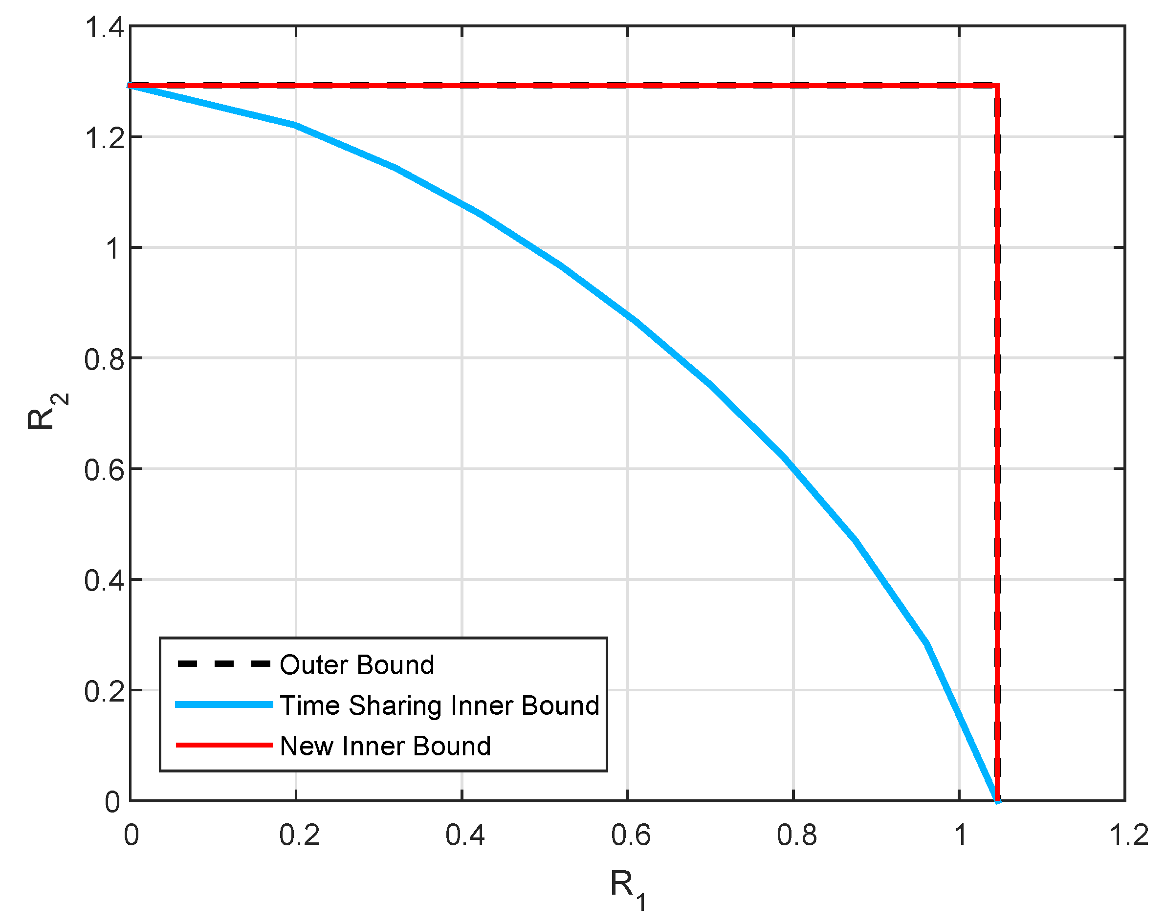
In practical situations the channel parameters
a and
b are fixed but the helper can control
. The results here imply that for a fixed
we can choose
such that the capacity gap is close to zero. We emphasize this in
Figure 10, where we plot the inner and outer bounds on achievable
with the following channel parameters
4. MIMO Gaussian Channel with Independent States
In this section, we consider the problem of channel coding over MIMO Gaussian parallel state-dependent channel with a cognitive helper where the states are independent. We start with deriving an achievable region for a general discrete memoryless case. We then, evaluate this region for the Gaussian setting by choosing an appropriate jointly Gaussian input distribution.
4.1. Problem Formulation
Consider a 3-transmitter, 2-receiver
state-dependent parallel DMC depicted in
Figure 11, where Transmitter 1 wishes to communicate a message
to Receiver 1, and similarly Transmitter 2 wishes to transmit a message
to its corresponding Receiver 2. The messages
and
are independent. The communication takes over a parallel state-dependent channel characterized by a probability transition matrix
. The transmitter at the helper has non-causal knowledge of the state and tries to mitigate the interference caused in both channels. The state variable
is random taking values in
and drawn from a discrete memoryless source (DMS)
A code for the parallel state-dependent channel with state known non-causally at the helper consists of
two message sets and ,
three encoders, where the encoder at the helper assigns a codeword to each state sequence , encoder 1 assigns a codeword to each message and encoder 2 assigns a codeword to each message , and
two decoders, where decoder 1 assigns an estimate or an error message e to each received sequence , and decoder 2 assigns an estimate or an error message e to each received sequence .
We assume that the message pair
is uniformly distributed over
. The average probability of error for a length-
n code is defined as
A rate pair is said to be achievable if there exists a sequence of codes such that . The capacity region is the closure of the set of all achievable rate pairs .
We observe that due to the lack of cooperation between the receivers, the capacity region of this channel depends on the
only through the conditional marginal PMFs
and
. This observation is similar to the DM-BC ([
37], Lemma 5.1).
Our goal is to characterize the capacity region
for the state-dependent Gaussian parallel channel with additive state known at the helper. Here, the state
. The channel is modeled by a Gaussian vector parallel state-dependent channel
where
,
are
channel gain matrices.
,
,
are the helper and the noncognitive transmitters channel input signals, each subject to an average matrix power constraint
The additive state variables and noise are independent and identically distributed (i.i.d.) Gaussian with zero mean and strictly positive definite covariance matrix and I respectively.
4.2. Outer and Inner Bounds
To characterize the capacity region of this channel, we first consider the following outer bound on the capacity region for the Gaussian setting.
Proposition 4. Every achievable rate pair of the state-dependent parallel Gaussian channel with a helper must satisfy the following inequalitiesfor and some covariance matrices , such that , where The proof of this outer bound is quite similar to the proof of the outer bound in Proposition 3 and is given in
Appendix D.
The upper bound for each rate consists of two terms, the first one reflects the scenario when the interference cannot be completely canceled, and the second is simply the point-to-point capacity of the channel without the state. Furthermore, the individual rate bounds are connected through the choice of and .
We next derive an achievable region for the channel based on an achievable scheme that integrates Marton’s coding, single-bin dirty paper coding, and state cancelation. More specifically, we generate two auxiliary random variables, and to incorporate the state information so that Receiver 1 (and respectively 2) decodes (and respectively ) and then decodes the respective transmitter information. Based on such an achievable scheme, we derive the following inner bound on the capacity region for the DM case.
Proposition 5. An inner bound on the capacity region of the discrete memoryless parallel state-dependent channel with a helper consists of rate pairs satisfying:for some PMF . Remark 1. The achievable region in Proposition 5 is equivalent to the following regionfor some PMF . Proof. The proof of the inner bound is relegated to
Appendix E. □
We evaluate the latter inner bound for the Gaussian channel by choosing the joint Gaussian distribution for random variables as follows:
where
are independent. For simplicity of representation, denote
,
and
. Let
and
be defined as
where the mutual information terms are evaluated using the joint Gaussian distribution set at (
29). Based on those definitions we obtain an achievable region for the Gaussian channel.
Proposition 6. An inner bound on the capacity region of the parallel state-dependent Gaussian channel with a helper and with independent states, consists of rate pairs satisfying;for some real matrices , , , , , and satisfying , . Now we provide our intuition behind such construction of the RVs in the proof of Proposition 6. contains two parts, the one with , controls the direct state cancelation of each state. The second part , , is used for dirty paper coding via generation of the state-correlated auxiliary RVs and .
4.3. Capacity Region Characterization
In this section, we will characterize segments on the capacity boundary for various channel parameters using the inner and outer bounds that were derived in
Section 4.2. Consider the inner bounds in (
30a)–(
30b). Each bound has two terms in the argument of min. We suggest optimizing each term independently and then comparing it to the outer bounds in (
25). In the last step we will state the conditions under which those terms are valid. Our technique for optimal choice of
be such that cancels the respective interfering terms from the mutual information quantities. We explain how those matrices were chosen in
Appendix F.
We begin by considering what choice of
can maximize
. Let
Then
takes the following form
If
, then
is achievable. Moreover, if we choose
, then
meets the outer bound (the first term in “min” in (
25)) with
and
. Furthermore, by setting
we obtain
If
, then
is achievable. Similarly, by choosing
, then
is achievable and this meets the outer bound (the second term in “min” in (
25)). Next we consider the bound on
. Let
Then
takes the following form
If
, then
is achievable. Moreover, if we choose
, then
meets the outer bound (the first term in “min” in (
25)).
Furthermore, we set
and then obtain
If , then is achievable and this meets the outer bound. This also equals the maximum rate for when the channel is not corrupted by state.
Summarizing the above analysis, we obtain the following characterization of segments of the capacity region boundary.
Theorem 3. The channel parameters can be partitioned into the sets , where If , then captures one segment of the capacity region boundary, where the state cannot be fully canceled. If , then captures one segment of the capacity region boundary where the state is fully canceled. If , then the segment of the capacity region boundary is not characterized.
The channel parameters can also be partitioned into the sets , where If , then captures one segment of the capacity region boundary, where the state cannot be fully canceled. If , then captures one segment of the capacity boundary where the state is fully canceled. If , then the segment of the capacity region boundary is not characterized.
The above theorem describes two partitions of the channel parameters, respectively under which segments on the capacity region boundary corresponding to and can be characterized. Intersection of two sets, each from one partition, collectively characterizes the entire segments on the capacity region boundary.
We note that our inner bound can be tight for some set of channel parameters. As an example, assume that
. In such case,
and
are achievable. For the point-to-point helper channel [
28], it was shown that if the helper power is above some threshold, the state is completely canceled, whereas in our model we have two parallel channels. If the helper power is high enough, it can split its signal, similarly as for the Gaussian BC, such that one part of it is intended for Receiver 2, where by using dirty paper coding it eliminates completely the interference caused by the state and the part of the signal intended for Receiver 1. In the same time the part of the helper signal intended for Receiver 1, can only cancel the interference caused by the state while the part intended to Receiver 2 is treated as noise.
4.4. Numerical Results
In this section, we provide specific numerical examples to illustrate the bounds obtained in the previous sections. In particular, we focus on scalar Gaussian channel setting, such that:
;
;
;
;
;
;
,
;
. We also denote
. We plot the inner and outer bounds for various values of helper power
, channel gains,
and
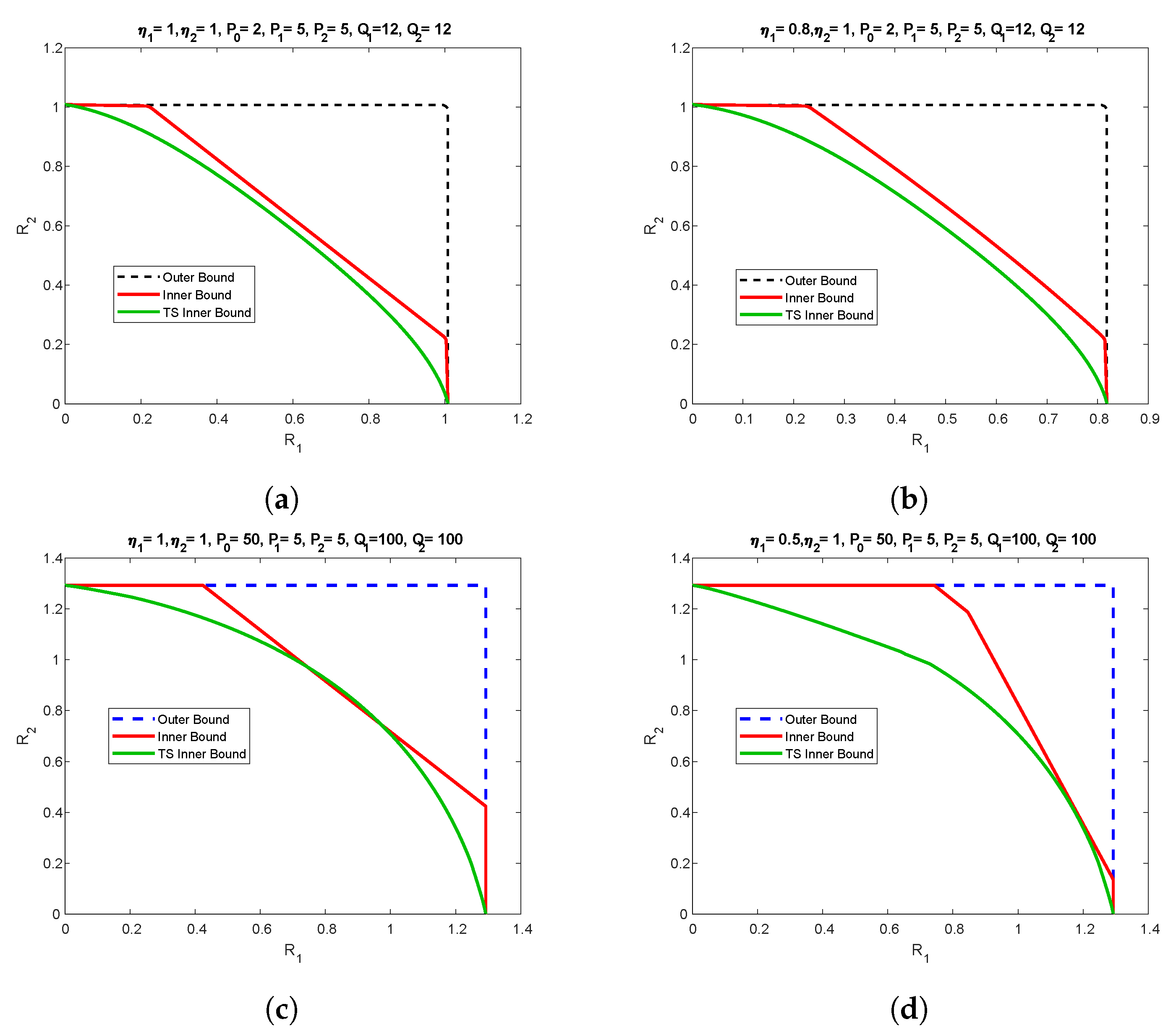
and different state power. The results are shown in
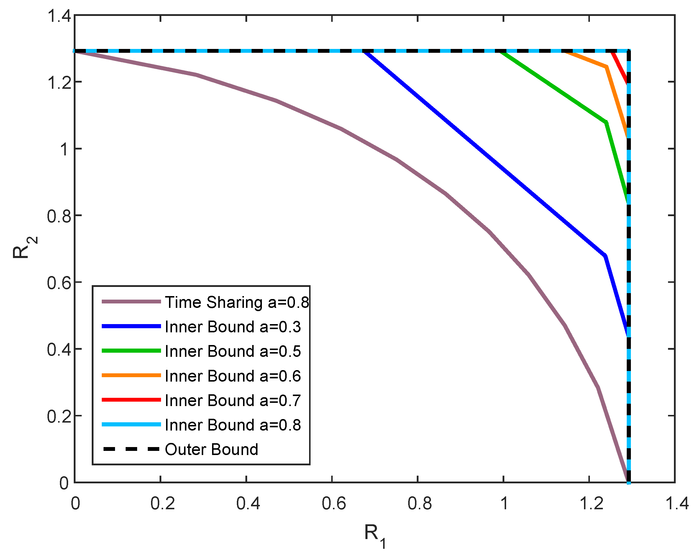
Figure 12. The outer bound is based on Proposition 4. The inner bound is the convex hull of all the achievable regions, with interchange between the roles of the decoders. The time-sharing inner bound is according to point-to-point helper channel achievable region [
28]. The scenario where the helper power is less than the users power is depicted in
Figure 12a,b, while the channel gains in
Figure 12a are equal, they are mismatched in
Figure 12b. Please note that in both cases our inner bound outperforms the time-sharing bound, especially in the mismatched case, and some segments of the capacity region are characterized.
The scenario with helper power being higher than the user power and matched and mismatched channel gain is depicted in
Figure 12c,d respectively. Similar to for low helper power regime, our proposed achievability scheme performs better than time-sharing.
5. Conclusions
In the first part of this paper, we have studied the parallel state-dependent Gaussian channel with a state-cognitive helper and with same but differently scaled states. An inner bound was derived and was compared to an upper bound, and the segments of the capacity region boundary were characterized for various channel parameters. We have shown that if the channel gain matrices satisfy a certain symmetry property, the full rectangular capacity region of the two point-to-point channels without the state can be achieved. Furthermore, for the scalar channel case, we have shown that for a given ratio of state gain over the helper signal gain, , one can find a value of the helper power—, such that the capacity region is fully characterized.
A different model of the parallel state-dependent Gaussian channel with a state-cognitive helper and independent states was considered in the second part of this study. Inner and outer bounds were derived, and segments of the capacity region boundary were characterized for various channel parameters. We have also demonstrated our results using numerical simulation and have shown that our achievability scheme outperforms time-sharing that was shown to be optimal for the infinite state power regime in [
34].
These two models represent a special case of a more general scenario with correlated states, our results in both studies imply that as the states get more correlated, it is easier to mitigate the interference. Furthermore, the gap between the inner bound and the outer bound in this work suggests that a new techniques for outer bound derivation is needed as we believe that the inner bounds consisting of pairs is indeed tight for some set of channel parameters.


.png)


