Informed Weighted Non-Negative Matrix Factorization Using αβ-Divergence Applied to Source Apportionment

 , , , and
Abstract
1. Introduction
- The entries of G and F are non-negative (one cannot assume a negative mass in G nor a negative proportion of chemical species in F).
- The product must fit the data matrix X.
- When one entry of the product does not fit the entry , we should then checki.e., the estimated mass of a chemical species in a sample should not be above the corresponding measured one.
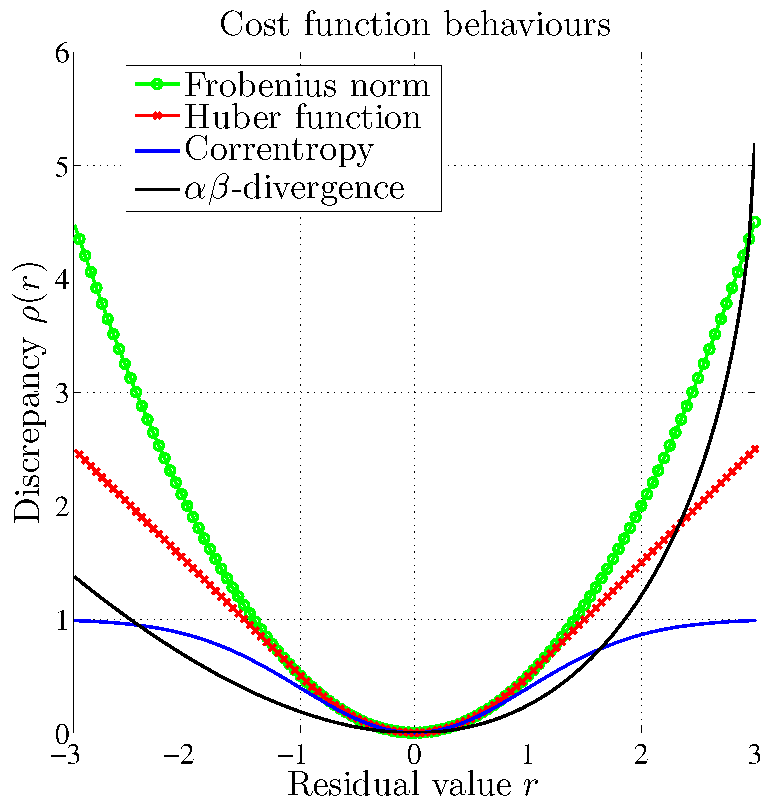
2. Robust Cost Functions
2.1. Introduction to Modified Cost Functions
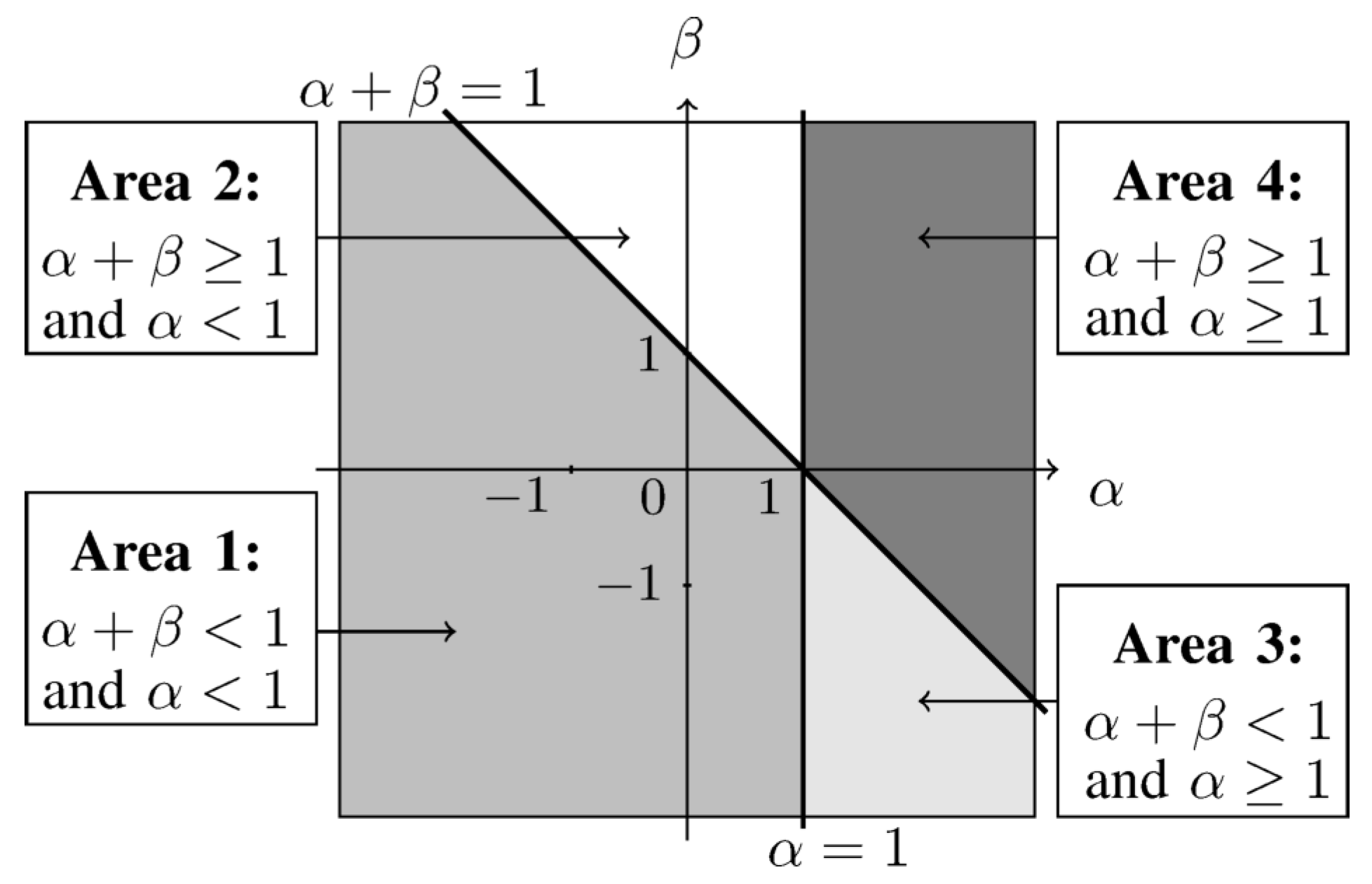
2.2. -Divergence
2.3. Existing NMF Methods with Parametric Divergences
3. Constraint Parameterization
4. General Problem Formulation
5. Proposed Informed -NMF Methods
5.1. Weighted -NMF with Set Constraints
5.2. Normalization Procedures
5.2.1. Classical Normalization
5.2.2. Alternative Normalization
5.2.3. Description of Algorithm Acronyms
| Algorithm 1-N-constrained weighted non-negative matrix factorization (CWNMF) residual (-R) method. |
| while do Update F at fixed G according to Equation (52) or (56) Update G at fixed F according to Equation (12) or (53) end while |
5.3. Bound-Constrained Normalized and Weighted -NMF
- the bound constraint projection followed by a normalization stage,
- or the normalization followed by the projection.
5.3.1. Informed NMF with Bound Constraints and Normalization
| Algorithm 2-BN-CWNMF method |
| while do Update F at fixed G according to Equation (61) Update G at fixed F according to Equation (62) end while |
5.3.2. Informed NMF with Normalization and Bound Constraints
| Algorithm 3-NB-CWNMF method |
| while do Update F at fixed G according to Equation (64) Update G at fixed F according to Equation (62) end while |
6. Experimental Results
6.1. Realistic Simulations
6.1.1. Source Profiles
6.1.2. Equality Constraints
6.1.3. Initialization
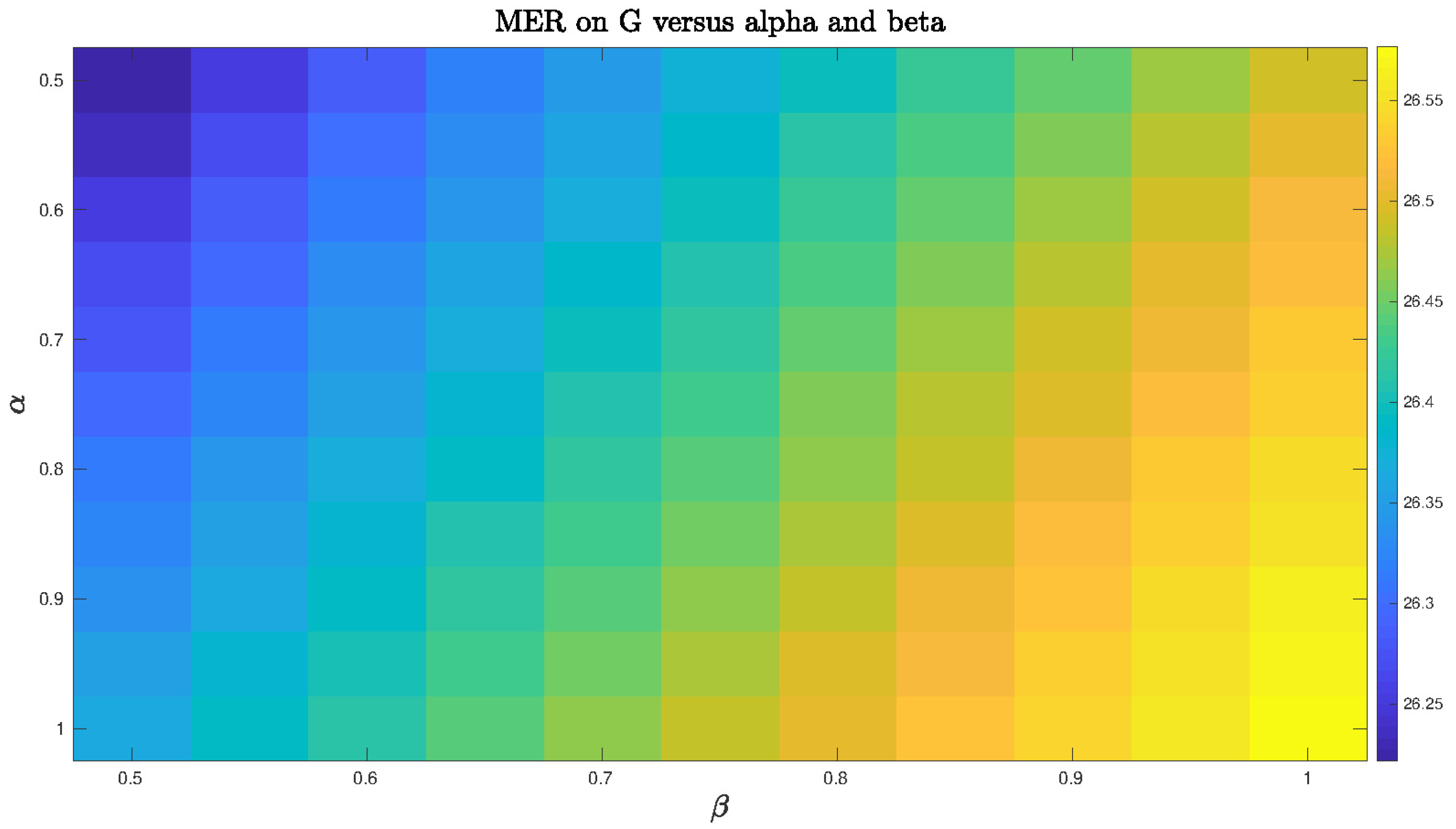
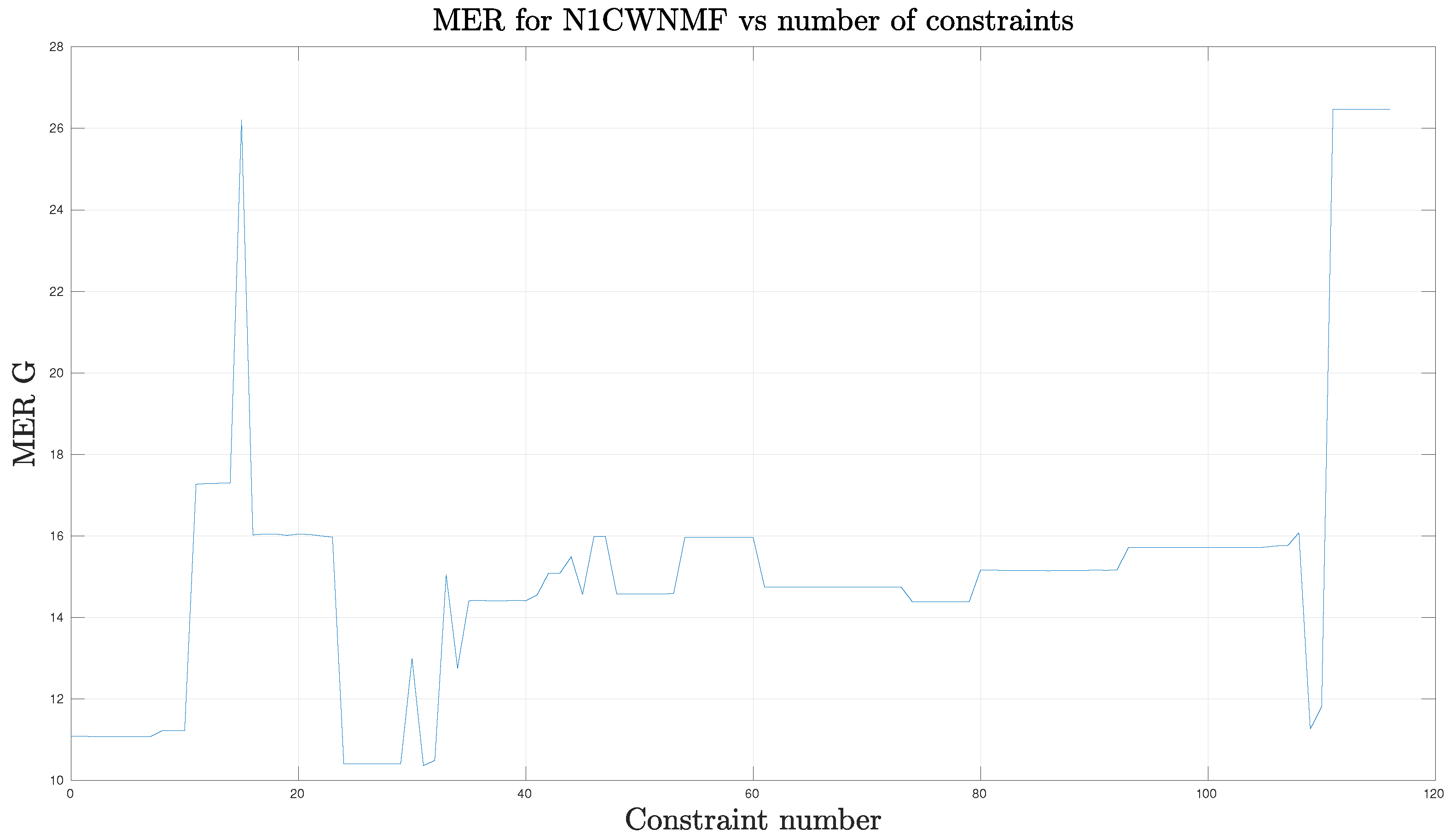
6.1.4. Performance Evaluation
6.2. Real Data Case
6.2.1. Context
6.2.2. Input Data
6.2.3. Results Evaluation
- Data are corrupted by an unknown number of outliers. Their origin may be of various kinds, e.g., the presence of a new source which affects the data at some sparse moments.
- Data are very noisy. In particular, an additional overall pollution—whose level highly varies over time—can not be assigned to a particular source and can significantly decrease the overall SNR.
- Some source profiles may be geometrically close, only a few tracer species are able to distinguish them.
7. Conclusions
Author Contributions
Funding
Acknowledgments
Conflicts of Interest
Abbreviations
| CWNMF | Constrained and weighted NMF |
| KKT | Karush–Kuhn Tucker |
| EC | Elementary carbon |
| MER | Mixing-error ratio |
| MM | Majorization-minimization |
| NMF | Non-negative matrix factorization |
| OC | Organic carbon |
| PM | Particulate matter |
| RNMF | Robust NMF |
| SIR | Signal-to-interference ratio |
| SNR | Signal-to-noise ratio |
| WNMF | Weighted NMF |
Appendix A. Update Rules for Problem (29)
Appendix B. Operating Conditions for the Simulations

| Profiles | Al | Cr | Fe | Mn | P | Sr | Ti | Zn | V | Ni | Co | Cu | Cd | Sb |
|---|---|---|---|---|---|---|---|---|---|---|---|---|---|---|
| Sea | 0.0019 | 0 | 0 | 0 | 2.5 | 0.2034 | 0 | 0 | 0 | 0 | 0 | 0 | 0 | 0 |
| Aged sea | 0 | 7.2351 | 0 | 0 | 0.5 | 0.4 | 1.877 | 0 | 0 | 0 | 1.785 | 1.7941 | 0 | 0 |
| Crustal | 119.13 | 8.589 | 77.35 | 1.782 | 3.0680 | 0.7846 | 8.9121 | 1.868 | 0.3503 | 0 | 0.0276 | 0.0081 | 0 | 0 |
| nitrates | 4.00 | 2 | 3.5 | 0.11 | 0.0749 | 0 | 0 | 0.7742 | 0 | 0 | 7.0408 | 0.1 | 6.486 | 0.01975 |
| sulfate | 0 | 5 | 0 | 0.02825 | 0.05313 | 0 | 0 | 0.1334 | 0 | 0 | 0.003287 | 8.00 | 0 | 0 |
| Biomass | 0.001 | 0 | 2.554 | 0.05527 | 0 | 1.016 | 0 | 0.1415 | 0 | 0 | 0 | 0 | 0 | 0.0385 |
| Road traffic | 0 | 0 | 39.0414 | 0.1404 | 2.659 | 0 | 0 | 10.908 | 0 | 0 | 1.00 | 2.7712 | 0 | 0.8964 |
| Sea traffic | 0.001147 | 1.2012 | 0.1002 | 0 | 0 | 0.0217 | 9.42 | 0 | 7.4920 | 5.5348 | 0.1829 | 1.752 | 1.315 | 0 |
| Biogenic | 0 | 0 | 0 | 0 | 14.528 | 0.04308 | 8.941 | 0 | 0 | 0 | 0 | 0 | 0 | 5.2 |
| Metal | 64.430 | 33.332 | 780.16 | 33 | 0.7 | 2 | 0 | 0 | 0 | 10 | 0.15 | 1.5 | 1.55 | 0 |
| Bis | OC | EC | Levo. | Polyols | ||||||||||
| Sea | 0 | 0 | 297.03 | 0 | 10.71 | 32.75 | 9.183 | 581.02 | 0 | 69.08 | 0 | 0 | 0 | 0 |
| Aged sea | 0 | 0.1 | 280 | 0 | 4 | 30 | 10 | 1.00 | 395 | 150 | 30 | 0 | 0 | 0 |
| Crustal | 0.0594 | 0 | 1.8333 | 4.36 | 5 | 5 | 301.81 | 0 | 49.95 | 39.96 | 384.92 | 0 | 0 | 0 |
| nitrates | 7.178 | 0.2075 | 0 | 216.26 | 3.2 | 0 | 0 | 1.21 | 730.73 | 0 | 45 | 0 | 0 | 9.027 |
| sulfate | 0 | 0.0729 | 0 | 260.83 | 4.43 | 0 | 0 | 8.66 | 0 | 680.59 | 53.84 | 0 | 0 | 0 |
| Biomass | 0 | 0.1007 | 2.650 | 2.85 | 12.26 | 0.001 | 11.67 | 25.48 | 35.16 | 56.84 | 692.10 | 91.14 | 69.78 | 1.477 |
| Road traffic | 0.0121 | 3.353 | 0 | 5.14 | 39.84 | 0 | 3.00 | 3.40 | 50.19 | 60.22 | 301.13 | 488.81 | 0 | 0 |
| Sea traffic | 0.0941 | 0 | 0 | 0.0626 | 0 | 0 | 0 | 0 | 75.17 | 300.69 | 500.76 | 109.87 | 0 | 0 |
| Biogenic | 0 | 0 | 5.023 | 0.0968 | 29.056 | 0 | 0 | 0.2975 | 0 | 20.094 | 854.02 | 0 | 0 | 76.83 |
| Metal | 0.2215 | 22.95 | 0 | 0 | 0 | 0 | 0 | 0 | 0 | 50.00 | 0 | 0 | 0 | 0 |
| Al | Cr | Fe | Mn | P | Sr | Ti | Zn | V | Ni | Co | Cu | Cd | Sb | |
|---|---|---|---|---|---|---|---|---|---|---|---|---|---|---|
| Sea | 0 | 1 | 1 | 1 | 0 | 0 | 1 | 1 | 1 | 1 | 1 | 1 | 1 | 1 |
| Aged sea | 1 | 0 | 1 | 1 | 0 | 0 | 0 | 1 | 1 | 1 | 0 | 0 | 1 | 1 |
| Crustal | 0 | 0 | 0 | 0 | 0 | 0 | 0 | 0 | 0 | 1 | 0 | 0 | 1 | 1 |
| nitrates | 0 | 0 | 0 | 0 | 0 | 1 | 1 | 0 | 1 | 1 | 0 | 0 | 0 | 0 |
| sulfate | 1 | 0 | 1 | 0 | 0 | 1 | 1 | 0 | 1 | 1 | 0 | 0 | 1 | 1 |
| Biomass | 0 | 1 | 0 | 0 | 1 | 0 | 1 | 0 | 1 | 1 | 1 | 1 | 1 | 0 |
| Road traffic | 1 | 1 | 0 | 0 | 0 | 1 | 1 | 0 | 1 | 1 | 0 | 0 | 1 | 0 |
| Sea traffic | 0 | 0 | 0 | 1 | 1 | 0 | 0 | 1 | 0 | 0 | 0 | 0 | 0 | 1 |
| Biogenic | 1 | 1 | 1 | 1 | 0 | 0 | 0 | 1 | 1 | 1 | 1 | 1 | 1 | 0 |
| Metal | 0 | 0 | 0 | 0 | 0 | 0 | 1 | 1 | 1 | 0 | 0 | 0 | 0 | 1 |
| La | Pb | Na | NH | K | Mg | Ca | Cl | NO | SO | OC | EC | Levo. | Polyols | |
| Sea | 1 | 1 | 0 | 1 | 0 | 0 | 0 | 0 | 1 | 0 | 1 | 0 | 1 | 1 |
| Aged sea | 1 | 0 | 0 | 1 | 0 | 0 | 0 | 0 | 0 | 0 | 0 | 1 | 1 | 1 |
| Crustal | 0 | 0 | 0 | 0 | 0 | 0 | 0 | 1 | 0 | 0 | 0 | 1 | 1 | 1 |
| nitrates | 0 | 0 | 1 | 0 | 0 | 0 | 1 | 0 | 0 | 1 | 0 | 0 | 1 | 0 |
| sulfate | 1 | 0 | 1 | 0 | 0 | 0 | 1 | 0 | 1 | 0 | 0 | 0 | 1 | 1 |
| Biomass | 1 | 0 | 0 | 0 | 0 | 0 | 0 | 0 | 0 | 0 | 0 | 0 | 0 | 0 |
| Road traffic | 0 | 0 | 1 | 0 | 0 | 1 | 0 | 0 | 0 | 0 | 0 | 0 | 1 | 1 |
| Sea traffic | 0 | 0 | 1 | 0 | 1 | 0 | 1 | 0 | 0 | 0 | 0 | 0 | 1 | 1 |
| Biogenic | 1 | 1 | 0 | 0 | 0 | 0 | 1 | 0 | 0 | 0 | 0 | 1 | 1 | 0 |
| Metal | 0 | 0 | 1 | 0 | 1 | 0 | 1 | 1 | 1 | 0 | 1 | 1 | 1 | 1 |
| Al | Cr | Fe | Mn | P | Sr | Ti | Zn | V | Ni | Co | Cu | Cd | Sb | |
|---|---|---|---|---|---|---|---|---|---|---|---|---|---|---|
| Sea | 0.2 | 1.00 | 1.00 | 1.00 | 0.01 | 0.8 | 1.00 | 1.00 | 1.00 | 1.00 | 1.00 | 1.00 | 1.00 | 1.00 |
| Aged sea | 1.00 | 0.001 | 1.00 | 1.00 | 1 | 1 | 0.01 | 1.00 | 1.00 | 1.00 | 0.01 | 0.01 | 1.00 | 1.00 |
| Crustal | 200 | 0.001 | 150 | 2 | 2 | 2 | 20 | 2 | 2 | 1.00 | 0.001 | 0.0001 | 1.00 | 1.00 |
| nitrates | 1.00 | 2.00 | 8 | 1 | 0.4 | 1.00 | 1.00 | 4 | 1.00 | 1.00 | 0.001 | 0.5 | 0.01 | 0.2 |
| sulfate | 1.00 | 1.00 | 1.00 | 1.00 | 0.5 | 1.00 | 1.00 | 0.4 | 1.00 | 1.00 | 0.01 | 1.00 | 1.00 | 1.00 |
| Biomass | 5 | 1.00 | 10 | 2 | 9.43 | 0.001 | 1.00 | 1 | 1.00 | 1.00 | 1.00 | 1.00 | 1.00 | 1.006 |
| Road traffic | 1.00 | 1.00 | 50 | 1 | 1.00 | 1.00 | 1.00 | 24 | 1.00 | 1.00 | 1.00 | 4 | 1.00 | 2 |
| Sea traffic | 0.01 | 1.00 | 0.4 | 1.00 | 1.00 | 0.1 | 1.00 | 1.00 | 18 | 10 | 1 | 1.00 | 1.00 | 1.00 |
| Biogenic | 1.00 | 1.00 | 1.00 | 1.00 | 5 | 7.96 | 7.96 | 1.00 | 1.00 | 1.00 | 1.00 | 1.00 | 1.00 | 7.96 |
| Metal | 73 | 70 | 650 | 50 | 3 | 5 | 1.00 | 1.00 | 1.00 | 30 | 1 | 3 | 4 | 1.00 |
| La | Pb | Na | NH | K | Mg | Ca | Cl | NO | SO | OC | EC | Levo. | Polyols | |
| Sea | 1.00 | 1 | 320 | 5 | 10 | 38 | 11 | 550 | 1 | 70 | 1 | 1 | 9.98 | 9.98 |
| Aged sea | 1.00 | 0.01 | 250 | 1 | 1 | 40 | 15 | 150 | 320DA80.eps | 210 | 12 | 1.00 | 9.99 | 9.99 |
| Crustal | 0.0001 | 1 | 0.0001 | 0.0001 | 10 | 10 | 250 | 1.00 | 30 | 30 | 290 | 1.00 | 1.00 | 1.00 |
| nitrates | 0.2 | 0.5 | 1 | 300 | 5 | 1.00 | 1.00 | 0.2 | 600 | 1.00 | 80 | 1.00 | 1.00 | 1.00 |
| sulfate | 1.00 | 0.1 | 1.00 | 305 | 10 | 1.00 | 1.00 | 1.00 | 1.00 | 584 | 100 | 1.00 | 1.00 | 1 |
| Biomass | 1.00 | 1 | 3 | 28 | 72 | 5 | 38 | 66 | 66 | 66 | 510 | 70 | 57 | 9.43 |
| Road traffic | 1 | 9.99 | 1.00 | 1.00 | 57 | 0.00049 | 1.00 | 1.00 | 79.99 | 80 | 260 | 430 | 9.99 | 9.99 |
| Sea traffic | 0.5 | 1.00 | 1 | 1.00 | 1 | 1 | 1.00 | 1 | 110 | 250 | 450 | 160 | 8.37 | 8.37 |
| Biogenic | 1.00 | 7.96 | 1 | 1 | 9 | 4 | 1.00 | 7.96 | 5 | 5 | 800 | 1 | 7.96 | 170 |
| Metal | 1 | 40 | 1.00 | 1.00 | 1.00 | 1.00 | 1.00 | 0.005 | 0.001 | 70 | 0.00164 | 1.64 | 1.64 | 1.64 |
Appendix C. Real Data Operating Conditions
| Al | Cr | Fe | Mn | P | Sr | Ti | Zn | V | Ni | Co | Cu | Cd | Sb | |
|---|---|---|---|---|---|---|---|---|---|---|---|---|---|---|
| Sea | 0.19 | 1.00 | 8.00 | |||||||||||
| Aged sea | 0.10 | 0.01 | 0.50 | 0.01 | 1.00 | 8.00 | 0.02 | 0.02 | 1.00 | 0.01 | 0.01 | 0.01 | ||
| Crustal | 266.67 | 0.14 | 150 | 2.00 | 2.00 | 20 | 0.50 | 0.50 | 0.07 | 0.07 | 0.07 | 0.01 | ||
| nitrates | 0.98 | 0.98 | 30 | 0.98 | 0.98 | 0.98 | 20 | 0.98 | 0.98 | 10 | 0.98 | 0.98 | ||
| sulfate | 1.00 | 1.00 | 30 | 1.00 | 1.00 | 15.00 | 20 | 1.00 | 1.00 | 1.00 | 1.00 | 1.00 | ||
| Biomass | 4.00 | 9.00 | 1.00 | 1.00 | 1.00 | 10 | 1.00 | |||||||
| Road traffic | 20 | 1.00 | 50 | 5.00 | 1.00 | 50 | 5.00 | 10 | 5.00 | 50 | 5.00 | 50 | ||
| Sea traffic | 10 | 10 | 5.00 | 55.00 | 55.00 | 30 | ||||||||
| Biogenic | 0.01 | 0.01 | 20 | 1.00 | ||||||||||
| Metal | 80 | 80 | 358 | 40 | 8 | 18.00 | 40 | 40 | 30 | 30 | 1.00 | 40 | 50 | 30 |
| La | Pb | Na | NH | K | Mg | Ca | Cl | NO | SO | OC | EC | Levo. | Polyols | |
| Sea | 320.00 | 10.00 | 40.00 | 10.00 | 540.08 | 70.00 | 0.64 | 0.09 | ||||||
| Aged Sea | 0.01 | 250.00 | 10.00 | 25.00 | 10.00 | 200.00 | 275.30 | 210.00 | 8.00 | 1.00 | ||||
| Crustal | 0.14 | 10.00 | 3.00 | 100.00 | 70.14 | 210.00 | 7.00 | 20.00 | 35.07 | 90.00 | 12.62 | |||
| nitrates | 0.98 | 200.00 | 0.98 | 0.98 | 40.00 | 0.98 | 547.30 | 100.00 | 40.00 | |||||
| sulfate | 20.00 | 200.00 | 34.00 | 1.00 | 40.00 | 1.00 | 554.00 | 60.00 | 16.00 | |||||
| Biomass | 0.00 | 0.94 | 2.83 | 28.31 | 70.00 | 4.72 | 37.74 | 66.05 | 70.00 | 66.05 | 500.61 | 69.29 | 56.46 | |
| Road traffic | 10.00 | 10.00 | 10.00 | 21.00 | 2.00 | 80.00 | 40.00 | 271.73 | 303.27 | |||||
| Sea traffic | 15.00 | 10.00 | 10.00 | 20.00 | 10.00 | 30.00 | 580.00 | 160.00 | ||||||
| Biogenic | 1.00 | 1.00 | 5.00 | 4.00 | 1.00 | 5.00 | 5.00 | 760.00 | 50.00 | 146.98 | ||||
| Metal | 1.00 | 80.00 | 1.00 | 48.00 | 10.00 | 5.00 | 10.00 |
| Al | Cr | Fe | Mn | P | Sr | Ti | Zn | V | Ni | Co | Cu | Cd | Sb | |
|---|---|---|---|---|---|---|---|---|---|---|---|---|---|---|
| Sea | 0 | 1 | 0 | 1 | 0 | 0 | 1 | 1 | 1 | 1 | 1 | 1 | 1 | 1 |
| Aged sea | 0 | 0 | 0 | 0 | 0 | 0 | 0 | 0 | 1 | 1 | 0 | 0 | 0 | 0 |
| Crustal | 0 | 0 | 0 | 0 | 0 | 0 | 0 | 0 | 0 | 0 | 0 | 0 | 0 | 0 |
| nitrates | 0 | 0 | 0 | 0 | 0 | 0 | 0 | 0 | 1 | 0 | 0 | 0 | 0 | 0 |
| sulfate | 0 | 0 | 0 | 0 | 0 | 0 | 0 | 0 | 1 | 0 | 0 | 0 | 0 | 0 |
| Biomass | 0 | 1 | 0 | 0 | 0 | 0 | 0 | 0 | 1 | 1 | 0 | 0 | 0 | 0 |
| Road traffic | 0 | 0 | 0 | 0 | 0 | 0 | 0 | 0 | 0 | 0 | 0 | 0 | 0 | 0 |
| Sea traffic | 0 | 0 | 0 | 0 | 0 | 0 | 0 | 0 | 0 | 0 | 0 | 0 | 0 | 0 |
| Biogenic | 0 | 0 | 0 | 1 | 0 | 0 | 0 | 0 | 1 | 1 | 0 | 0 | 1 | 0 |
| Metal | 0 | 0 | 0 | 0 | 0 | 0 | 0 | 0 | 0 | 0 | 0 | 0 | 0 | 0 |
| La | Pb | Na | NH | K | Mg | Ca | Cl | NO | SO | OC | EC | Levo. | Polyols | |
| Sea | 1 | 1 | 0 | 1 | 0 | 0 | 0 | 0 | 1 | 0 | 0 | 0 | 1 | 1 |
| Aged sea | 0 | 0 | 0 | 1 | 0 | 0 | 0 | 0 | 0 | 0 | 0 | 0 | 1 | 1 |
| Crustal | 0 | 0 | 0 | 0 | 0 | 0 | 0 | 0 | 0 | 0 | 0 | 0 | 1 | 1 |
| nitrates | 0 | 0 | 1 | 0 | 0 | 0 | 0 | 0 | 0 | 1 | 0 | 0 | 1 | 0 |
| sulfate | 0 | 0 | 1 | 0 | 0 | 0 | 0 | 0 | 1 | 0 | 0 | 0 | 1 | 0 |
| Biomass | 0 | 0 | 0 | 0 | 0 | 0 | 0 | 0 | 0 | 0 | 0 | 0 | 0 | 0 |
| Road traffic | 0 | 0 | 1 | 0 | 0 | 1 | 0 | 0 | 0 | 0 | 0 | 0 | 1 | 1 |
| Sea Traffic | 0 | 0 | 1 | 0 | 0 | 0 | 0 | 0 | 0 | 0 | 0 | 0 | 1 | 1 |
| Biogenic | 1 | 1 | 0 | 0 | 0 | 0 | 0 | 0 | 0 | 0 | 0 | 0 | 1 | 0 |
| Metal | 0 | 0 | 1 | 0 | 0 | 0 | 0 | 1 | 1 | 0 | 1 | 1 | 1 | 1 |
| Al | Cr | Fe | Mn | P | Sr | Ti | Zn | V | Ni | Co | Cu | Cd | Sb | |
|---|---|---|---|---|---|---|---|---|---|---|---|---|---|---|
| Sea | 0 | 0 | 0 | 0 | 0 | 20/0 | 0 | 0 | 0 | 0 | 0 | 0 | 0 | 0 |
| Aged sea | 0 | 0 | 0 | 0 | 0 | 20/0 | 0 | 0 | 0 | 0 | 0 | 0 | 0 | 0 |
| Crustal | 400/50 | 0 | 200/1 | 0 | 0 | 0 | 40/0.001 | 0 | 0 | 0 | 0 | 0 | 0 | 0 |
| nitrates | 0 | 0 | 0 | 0 | 0 | 0 | 0 | 0 | 0 | 0 | 0 | 0 | 0 | 0 |
| sulfates | 0 | 0 | 0 | 0 | 0 | 0 | 0 | 0 | 0 | 0 | 0 | 0 | 0 | 0 |
| Biomass | 100/0.001 | 0 | 100/0.001 | 0 | 0 | 0 | 0 | 0 | 0 | 0 | 0 | 0 | 0 | 0 |
| Road traffic | 0 | 0 | 75/1 | 0 | 0 | 0 | 0 | 50/0.1 | 0 | 0 | 0 | 15/0.000001 | 0 | 15/0.000001 |
| Sea traffic | 0 | 0 | 70/0.1 | 0 | 0 | 0 | 0 | 0 | 70/5 | 70/5 | 50/0.00001 | 0 | 0 | 0 |
| Biogenic | 0 | 0 | 0 | 0 | 0 | 0 | 0 | 0 | 0 | 0 | 0 | 0 | 0 | 0 |
| Metal | 0 | 0 | 0 | 0 | 0 | 0 | 0 | 0 | 0 | 0 | 0 | 0 | 0 | 0 |
| La | Pb | Na | NH | K | Mg | Ca | Cl | NO | SO | OC | EC | Levo. | Polyols | |
| Sea | 0 | 0 | 400/200 | 0 | 50/5 | 50/15 | 50/5 | 720/360 | 0 | 100/30 | 0 | 0 | 0 | 0 |
| Aged sea | 0 | 0 | 0 | 0 | 0 | 0 | 0 | 250/0 | 500/50 | 500/50 | 0 | 0 | 0 | 0 |
| Crustal | 0 | 0 | 0 | 0 | 150/5 | 150/5 | 500/50 | 0 | 50/0 | 40/0 | 0 | 0 | 0 | 0 |
| nitrates | 0 | 0 | 0 | 800/50 | 0 | 0 | 0 | 0 | 950/200 | 0 | 0 | 0 | 0 | 0 |
| sulfates | 0 | 0 | 0 | 800/50 | 0 | 0 | 0 | 0 | 0 | 950/200 | 0 | 0 | 0 | 0 |
| Biomass | 0 | 0 | 10/0 | 40/0 | 100/1 | 5/0 | 100/0.001 | 100/0.001 | 150/1 | 150/0 | 750/100 | 200/5 | 0 | 0 |
| Road traffic | 0 | 0 | 0 | 20/0 | 0 | 0 | 0 | 10/0 | 60/10 | 80/20 | 300/150 | 800/250 | 0 | 0 |
| Sea Traffic | 30/0 | 0 | 0 | 20/0 | 0 | 0 | 0 | 20/0 | 75/0 | 300/10 | 700/100 | 200/50 | 0 | 0 |
| Biogenic | 0 | 0 | 5/0 | 5/0 | 0 | 0 | 0 | 5/0 | 5/0 | 20/0 | 850/500 | 0 | 0 | 0 |
| Metal | 0 | 0 | 0 | 0 | 0 | 0 | 0 | 0 | 0 | 60/10 | 0 | 0 | 0 | 0 |
References
- Hopke, P. Review of receptor modeling methods for source apportionment. J. Air Waste Manag. Assoc. 2016, 66, 237–259. [Google Scholar] [CrossRef] [PubMed]
- Paatero, P. The Multilinear Engine—A Table-Driven, Least Squares Program for Solving Multilinear Problems, Including the n-Way Parallel Factor Analysis Model. J. Comput. Graph. Stat. 1999, 8, 854–888. [Google Scholar] [CrossRef]
- Gillis, N. The why and how of nonnegative matrix factorization. In Regularization, Optimization, Kernels, and Support Vector Machines; Chapman and Hall/CRC: Palo Alto, CA, USA, 2014; pp. 257–291. [Google Scholar]
- Paatero, P.; Tapper, U. Positive matrix factorization: A non negative factor model with optimal utilization of error estimates of data values. Environmetrics 1994, 5, 111–126. [Google Scholar] [CrossRef]
- Parra, L.C.; Spence, C.; Sajda, P.; Ziehe, A.; Müller, K.R. Unmixing hyperspectral data. Adv. Neural Inf. Process. Syst. 2000, 12, 942–948. [Google Scholar]
- Zdunek, R. Regularized nonnegative matrix factorization: Geometrical interpretation and application to spectral unmixing. Int. J. Appl. Math. Comput. Sci. 2014, 24, 233–247. [Google Scholar] [CrossRef]
- Igual, J.; Llinares, R. Nonnegative matrix factorization of laboratory astrophysical ice mixtures. IEEE J. Sel. Top. Signal Process. 2008, 2, 697–706. [Google Scholar] [CrossRef]
- Berné, O.; Joblin, C.; Deville, Y.; Smith, J.; Rapacioli, M.; Bernard, J.; Thomas, J.; Reach, W.; Abergel, A. Analysis of the emission of very small dust particles from Spitzer spectro-imagery data using blind signal separation methods. Astron. Astrophys. 2007, 469, 575–586. [Google Scholar] [CrossRef]
- Gobinet, C.; Perrin, E.; Huez, R. Application of non-negative matrix factorization to fluorescence spectroscopy. In Proceedings of the 12th European Signal Processing Conference (EUSIPCO’04), Vienna, Austria, 6–10 September 2004; pp. 1095–1098. [Google Scholar]
- Févotte, C.; Vincent, E.; Ozerov, A. Single-channel audio source separation with NMF: Divergences, constraints and algorithms. In Audio Source Separation; Springer: Cham, Switzerland, 2018; pp. 1–24. [Google Scholar]
- Puigt, M.; Delmaire, G.; Roussel, G. Environmental signal processing: New trends and applications. In Proceedings of the 25th European Symposium on Artificial Neural Networks, Computational Intelligence and Machine Learning (ESANN’17), Bruges, Belgium, 26–28 April 2017; pp. 205–214. [Google Scholar]
- Hoyer, P. Non-negative matrix factorization with sparseness constraint. J. Mach. Learn. Res. 2004, 5, 1457–1469. [Google Scholar]
- Dorffer, C.; Puigt, M.; Delmaire, G.; Roussel, G. Informed Nonnegative Matrix Factorization Methods for Mobile Sensor Network Calibration. IEEE Trans. Signal Inf. Process. Netw. 2018, 4, 667–682. [Google Scholar] [CrossRef]
- Lantéri, H.; Theys, C.; Richard, C.; Févotte, C. Split Gradient Method for Nonnegative Matrix Factorization. In Proceedings of the 18th European Signal Processing Conference, Aalborg, Denmark, 23–27 August 2010. [Google Scholar]
- Meganem, I.; Deville, Y.; Hosseini, S.; Déliot, P.; Briottet, X. Linear-Quadratic Blind Source Separation Using NMF to Unmix Urban Hyperspectral Images. IEEE Trans. Signal Process. 2014, 62, 1822–1833. [Google Scholar] [CrossRef]
- Dorffer, C.; Puigt, M.; Delmaire, G.; Roussel, G. Nonlinear Mobile Sensor Calibration Using Informed Semi-Nonnegative Matrix Factorization with a Vandermonde Factor. In Proceedings of the 2016 IEEE Sensor Array and Multichannel Signal Processing Workshop (SAM), Rio de Janerio, Brazil, 10–13 July 2016. [Google Scholar]
- Yoo, J.; Choi, S. Nonnegative Matrix Factorization with Orthogonality Constraints. J. Comput. Sci. Eng. 2010, 4, 97–109. [Google Scholar] [CrossRef]
- Févotte, C.; Dobigeon, N. Nonlinear hyperspectral unmixing with robust nonnegative matrix factorization. IEEE Trans. Image Process. 2015, 24, 4810–4819. [Google Scholar] [CrossRef] [PubMed]
- Dhillon, S.; Sra, S. Generalized nonnegative matrix approximations with Bregman divergences. In Proceedings of the 18th International Conference on Neural Information Processing Systems, Vancouver, BC, Canada, 5–8 December 2005; pp. 283–290. [Google Scholar]
- Cichocki, A.; Lee, H.; Kim, Y.; Choi, S. Nonnegative matrix factorization with alpha-divergence. Pattern Recognit. Lett. 2008, 29, 1433–1440. [Google Scholar] [CrossRef]
- Févotte, C.; Idier, J. Algorithms for nonnegative matrix factoriaztion with the beta-divergence. Neural Comput. 2011, 23, 2421–2456. [Google Scholar] [CrossRef]
- Sun, D.; Fevotte, C. Alternating direction method of multipliers for non-negative matrix factorization with the beta-divergence. In Proceedings of the 2014 IEEE International Conference on Acoustics, Speech and Signal Processing (ICASSP), Florence, Italy, 4–9 May 2014; pp. 6201–6205. [Google Scholar]
- Cichocki, A.; Cruces, S.; Amari, S. Generalized Alpha-Beta divergences and their application to robust nonnegative matrix factorization. Entropy 2011, 13, 134–170. [Google Scholar] [CrossRef]
- Zhu, F.; Halimi, A.; Honeine, P.; Chen, B.; Zheng, N. Correntropy Maximization via ADMM—Application to Robust Hyperspectral Unmixing. IEEE Trans. Geosci. Remote Sens. 2017, 55, 1–12. [Google Scholar] [CrossRef]
- Chreiky, R.; Delmaire, G.; Puigt, M.; Roussel, G.; Abche, A. Informed split gradient Non-negative Matrix Factorization using Huber cost function for source apportionment. In Proceedings of the 2016 IEEE International Symposium on Signal Processing and Information Technology, Limassol, Cyprus, 12–14 December 2016. [Google Scholar]
- Paatero, P. Least squares formulation of robust non-negative factor analysis. Chemom. Intell. Lab. Syst. 1997, 37, 23–35. [Google Scholar] [CrossRef]
- Ho, N.D. Non Negative Matrix Factorization Algorithms and Applications. Ph.D. Thesis, Université Catholique de Louvain, Louvain-la-Neuve, Belgium, June 2008. [Google Scholar]
- Zhang, S.; Wang, W.; Ford, J.; Makedon, F. Learning from incomplete ratings using non-negative matrix factorization. In Proceedings of the 2006 SIAM International Conference on Data Mining, Bethesda, MD, USA, 20–22 April 2006; pp. 549–553. [Google Scholar]
- Dorffer, C.; Puigt, M.; Delmaire, G.; Roussel, G. Fast nonnegative matrix factorization and completion using Nesterov iterations. In Proceedings of the 13th International Conference on Latent Variable Analysis and Signal Separation, Grenoble, France, 21–23 February 2017; pp. 26–35. [Google Scholar]
- Viana, M.; Pandolfi, A.; Minguillo, M.C.; Querol, X.; Alastuey, A.; Monfort, E.; Celades, I. Inter-comparison of receptor models for PM source apportionment: Case study in an industrial area. Atmos. Environ. 2008, 42, 3820–3832. [Google Scholar] [CrossRef]
- Plouvin, M.; Limem, A.; Puigt, M.; Delmaire, G.; Roussel, G.; Courcot, D. Enhanced NMF initialization using a physical model for pollution source apportionment. In Proceedings of the 22nd European Symposium on Artificial Neural Networks, Computational Intelligence and Machine Learning (ESANN 2014), Brugge, Belgium, 23–25 April 2014; pp. 261–266. [Google Scholar]
- Limem, A.; Delmaire, G.; Puigt, M.; Roussel, G.; Courcot, D. Non-negative matrix factorization under equality constraints—a study of industrial source identification. Appl. Numer. Math. 2014, 85, 1–15. [Google Scholar] [CrossRef]
- Choo, J.; Lee, C.; Reddy, C.; Park, H. Weakly supervised nonnegative matrix factorization for user-driven clustering. Data Min. Knowl. Discov. 2015, 29, 1598–1621. [Google Scholar] [CrossRef]
- De Vos, M.; Van Huffel, S.; De Lathauwer, L. Spatially Constrained ICA Algorithm with an Application in EEG Processing. Signal Process. 2011, 91, 1963–1972. [Google Scholar] [CrossRef]
- Limem, A.; Delmaire, G.; Puigt, M.; Roussel, G.; Courcot, D. Non-negative matrix factorization using weighted beta divergence and equality constraints for industrial source apportionment. In Proceedings of the 2013 IEEE International Workshop on Machine Learning for Signal Processing (MLSP), Southampton, UK, 22–25 September 2013. [Google Scholar]
- Limem, A.; Puigt, M.; Delmaire, G.; Roussel, G.; Courcot, D. Bound constrained weighted NMF for industrial source apportionment. In Proceedings of the 2014 IEEE International Workshop on Machine Learning for Signal Processing (MLSP), Reims, France, 21–24 September 2014. [Google Scholar]
- Zhang, Z. Parameter estimation techniques: A tutorial with application to conic fitting. Image Vis. Comput. 1997, 15, 59–76. [Google Scholar] [CrossRef]
- Lee, D.; Seung, H. Learning the parts of objects by non negative matrix factorization. Nature 1999, 401, 788–791. [Google Scholar] [CrossRef] [PubMed]
- Lin, C.J. On the Convergence of Multiplicative Update Algorithms for Non-negative Matrix Factorization. IEEE Trans. Neural Netw. 2007, 18, 1589–1596. [Google Scholar]
- Hunter, D.R.; Lange, K. A tutorial on MM algorithms. Am. Stat. 2004, 58, 30–37. [Google Scholar] [CrossRef]
- Hennequin, R.; David, B.; Badeau, R. Beta-Divergence as a Subclass of Bregman Divergence. IEEE Signal Process. Lett. 2011, 18, 83–86. [Google Scholar] [CrossRef]
- Guillamet, D.; Vitria, J.; Schiele, B. Introducing a weighted non-negative matrix factorization for image classification. Pattern Recognit. Lett. 2003, 24, 2447–2454. [Google Scholar] [CrossRef]
- Xu, Y.; Yin, W.; Wen, Z.; Zhang, Y. An alternating direction algorithm for matrix completion with nonnegative factors. Front. Math. China 2012, 7, 365–384. [Google Scholar] [CrossRef]
- Heinz, D.C.; Chang, C. Fully constrained least squares linear mixture analysis for material quantification in hyperspectral imagery. IEEE Trans. Geosci. Remote Sens. 2001, 39, 529–545. [Google Scholar] [CrossRef]
- Lin, C.J. Projected Gradients Methods for Non-Negative Matrix Factorization. Neural Comput. 2007, 19, 2756–2779. [Google Scholar] [CrossRef] [PubMed]
- Moussaoui, S. Séparation de Sources Non-NéGatives. Application au Traitement des Signaux de Spectroscopie. Ph.D. Thesis, Université Henri Poincaré, Nancy, France, 2005. (In French). [Google Scholar]
- Roche, C.; Ledoux, F.; Borgie, M.; Delmaire, G.; Roussel, G.; Puigt, M.; Courcot, D. Origins of PM10 in northern coast of France: A one year study to estimate maritime contributions in the Strait of Dover. In Proceedings of the 22nd European Aerosol Conference, Tours, France, 4–9 September 2016. [Google Scholar]
- Kfoury, A. Origin and Physicochemical Behaviour of Atmospheric PM2.5 in Cities Located in the Littoral Area of the Nord-Pas-de-Calais Region, France. Ph.D. Thesis, Université du Littoral Côte d’Opale, Dunkerque, France, May 2013. [Google Scholar]
- Kfoury, A.; Ledoux, F.; Roche, C.; Delmaire, G.; Roussel, G.; Courcot, D. PM2.5 source apportionment in a French urban coastal site under steelworks emission influences using constrained non-negative matrix factorization receptor model. J. Environ. Sci. 2016, 40, 114–128. [Google Scholar] [CrossRef] [PubMed]
- Waked, A.; Favez, O.; Alleman, L.Y.; Piot, C.; Petit, J.E.; Delaunay, T.; Verlinden, E.; Golly, B.; Besombes, J.L.; Jaffrezo, J.L.; et al. Source apportionment of PM10 in a north-western Europe regional urban background site (Lens, France) using positive matrix factorization and including primary biogenic emissions. Atmos. Chem. Phys. 2014, 14, 3325–3346. [Google Scholar] [CrossRef]
- Becagli, S.; Sferlazzo, D.M.; Pace, G.; di Sarra, A.; Bommarito, C.; Calzolai, G.; Ghedini, C.; Lucarelli, F.; Meloni, D.; Monteleone, F.; et al. Evidence for heavy fuel oil combustion aerosols from chemical analyses at the island of Lampedusa: A possible large role of ships emissions in the Mediterranean. Atmos. Chem. Phys. 2012, 12, 3479–3492. [Google Scholar] [CrossRef]
- Vincent, E.; Araki, S.; Bofill, P. The 2008 Signal Separation Evaluation Campaign: A community-based approach to large-scale evaluation. In Proceedings of the 8th International Conference on Independent Component Analysis and Signal Separation (ICA 2009), Paraty, Brazil, 15–18 March 2009; pp. 734–741. [Google Scholar]
- Le Roux, J.; Hershey, J.R.; Weninger, F. Sparse NMF–Half-baked or Well Done? Technical Report TR2015-023; Mitsubishi Electric Research Labs (MERL): Cambridge, MA, USA, 2015. [Google Scholar]
- Roche, C. Etude des Concentrations et de la Composition des PM10 sur le Littoral du Nord de la France—Evaluation des Contributions Maritimes de L’espace Manche-Mer du Nord. Ph.D. Thesis, Université du Littoral Côte d’Opale, Dunkerque, France, 2016. [Google Scholar]
- Ledoux, F.; Roche, C.; Cazier, F.; Beaugard, C.; Courcot, D. Influence of ship emissions on NOx, SO2, O3 and PM concentrations in a North-Sea harbor in France. J. Environ. Sci. 2018, 71, 56–66. [Google Scholar] [CrossRef] [PubMed]


| small zoom | large zoom | |
| large zoom | small zoom |
| large weighting | small weighting | |
| small weighting | large weighting |
| Acronym | F | G | Mask on F | Mask on G |
|---|---|---|---|---|
| -N-CWNMF-R | Equation (52) | Equation (53) | ||
| -N-CWNMF | Equation (52) | Equation (53) | ||
| -N-CWNMF-R | Equation (56) | Equation (12) | ||
| -N-CWNMF | Equation (56) | Equation (12) |
| Profiles | Type | Major Species | References |
|---|---|---|---|
| Sea salts | Natural | , , , , , , | [48] |
| Crustal dust | Natural | , , , , OC, , , | [49] |
| Primary biogenic emission | Natural | OC, EC, Polyols, P | [50] |
| Aged sea salts | Anthropised | , , , , , OC, , , | [50] |
| Secondary nitrates | Anthropised | , OC, , EC, , , , | [50] |
| Secondary sulfates | Anthropised | , , OC, , , , , | [49] |
| Biomass combustion | Anthropogenic | OC, EC, Levoglucosan, , , | [50] |
| Road traffic | Anthropogenic | EC, OC, , , , , | [50] |
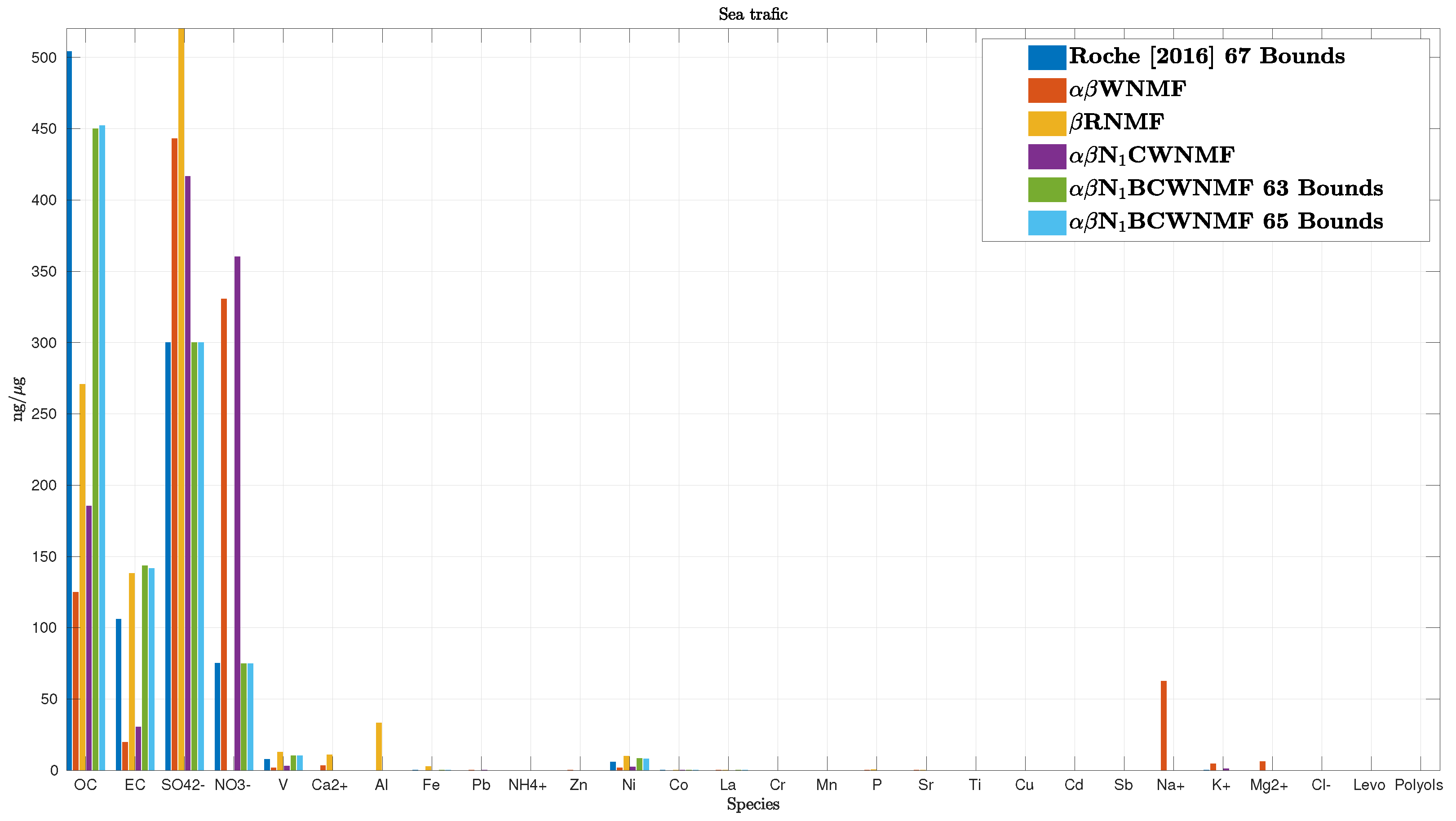
| Sea traffic | Anthropogenic | OC, EC, V, , , , , | [50,51] |
| Rich metal source | Anthropogenic | , , , , , | [50] |
© 2019 by the authors. Licensee MDPI, Basel, Switzerland. This article is an open access article distributed under the terms and conditions of the Creative Commons Attribution (CC BY) license (http://creativecommons.org/licenses/by/4.0/).
Share and Cite
Delmaire, G.; Omidvar, M.; Puigt, M.; Ledoux, F.; Limem, A.; Roussel, G.; Courcot, D. Informed Weighted Non-Negative Matrix Factorization Using αβ-Divergence Applied to Source Apportionment. Entropy 2019, 21, 253. https://doi.org/10.3390/e21030253
Delmaire G, Omidvar M, Puigt M, Ledoux F, Limem A, Roussel G, Courcot D. Informed Weighted Non-Negative Matrix Factorization Using αβ-Divergence Applied to Source Apportionment. Entropy. 2019; 21(3):253. https://doi.org/10.3390/e21030253
Chicago/Turabian StyleDelmaire, Gilles, Mahmoud Omidvar, Matthieu Puigt, Frédéric Ledoux, Abdelhakim Limem, Gilles Roussel, and Dominique Courcot. 2019. "Informed Weighted Non-Negative Matrix Factorization Using αβ-Divergence Applied to Source Apportionment" Entropy 21, no. 3: 253. https://doi.org/10.3390/e21030253
APA StyleDelmaire, G., Omidvar, M., Puigt, M., Ledoux, F., Limem, A., Roussel, G., & Courcot, D. (2019). Informed Weighted Non-Negative Matrix Factorization Using αβ-Divergence Applied to Source Apportionment. Entropy, 21(3), 253. https://doi.org/10.3390/e21030253